Perturbative Expansion of the Colored Jones Polynomial
Andrea Overbay
A dissertation submitted to the faculty of the University of North Carolina at Chapel Hill in partial fulfillment of the requirements for the degree of Doctor of Philosophy in the Department of Mathematics.
Chapel Hill 2013
Approved by:
Lev Rozansky
Prakash Belkale
Robert Lipshitz
Justin Sawon
Abstract
ANDREA OVERBAY: Perturbative Expansion of the Colored Jones Polynomial (Under the direction of Lev Rozansky)
Both the Alexander polynomial ∆K(t) and the colored Jones polynomialVα(K;q)
are well-known knot invariants. While the Jones polynomial seems similar to the
Alexander polynomial, it lacks an interpretation in classical topology. Because the
Alexander polynomial has a classical topological definition, exploring a relationship
between the two polynomials offers the possibility of interpreting the Jones polynomial
topologically.
Melvin and Morton conjectured a relationship between the two through an
expan-sion of the colored Jones polynomial [18]. The conjecture was proven by Bar-Natan
and Garoufalidis [4] and Rozansky extended the result further [24]. Rozansky proved
the following expansion inh =q−1:
Vα(K;q) = X
n≥0
hn
P(n)(K;qα/2−q−α/2)
∆2Kn+1(qα/2−q−α/2)
where P(n)(K;qα/2−q−α/2)∈
Z[qα, q−α] are polynomial invariants of the knot K.
In this dissertation, we will describe how we used the quantum group Uq(sl(2))
and techniques from quantum field theory to calculate the first two of these
polyno-mial invariants for all prime knots of up to nine crossings and present these results.
Furthermore, we will provide evidence of the validity of a conjecture from [23] by
calculating P(1)(K;qα/2−q−α/2) and P(2)(K;qα/2 −q−α/2) for all amphicheiral knots
Acknowledgements
I would like to thank my advisor, Dr. Lev Rozansky, for his direction, support,
and encouragement throughout this process. Without his assistance and guidance,
I would not have been able to complete this project. I would also like to thank
my committee members Dr. Prakash Belkale, Dr. Robert Lipshitz, Dr. Richard
Rimanyi, Dr. Justin Sawon, and Dr. Jonathan Wahl for their insight and advice. I
am also grateful to all of the University of North Carolina mathematics faculty for
their encouragement.
My family has been a constant support, and my accomplishments are a testament
to their unwavering love. Mom, Dad, Audria, and Jama, thank you. Included in my
family are those friends I have gained along the way. Damon, Rachel, Andrew, and
J.D., thank you. You have all been there when I needed you the most. Furthermore,
I must thank all of my fellow graduate students in the mathematics department for
their camaraderie.
Lastly, but certainly not least, I wish to thank the faculty at Emory and Henry
College for encouraging me to pursue a graduate career in mathematics. Dr. John
Table of Contents
List of Tables . . . vi
List of Figures . . . vii
Chapter 1. Introduction . . . 1
2. The Alexander Polynomial . . . 8
2.1. Preliminaries . . . 8
2.2. A Topological Definition of the Alexander Polynomial . . . 10
2.3. A Skein Relation Definition of the Alexander Polynomial . . . 12
2.4. Presenting Knots as Braid Closures . . . 13
2.5. The Alexander Polynomial by the Burau Representation . . . 15
3. The Jones Polynomial as the Quantum Trace of a Braid . . . 17
3.1. The Bracket Polynomial . . . 17
3.2. The Jones Polynomial . . . 18
3.3. The Quantum GroupUq(sl(2)) . . . 20
3.4. Calculating the Colored Jones Polynomial . . . 21
3.5. The Melvin-Morton-Rozansky Expansion . . . 22
4. Expansion of the R-matrix . . . 26
4.1. The h-adic Hopf Algebra Uh(sl(2)) . . . 26
4.2. The Generators E, F, and H . . . 29
4.3. Expansion ofRn(h) . . . 32
4.5. Expansion of exp(2hE⊗F) . . . 34
4.6. Expansion of exp(h(H⊗H)/2) . . . 37
4.7. Proof of Theorem 4.1.1 . . . 39
5. Composing Operators and Taking the Trace . . . 45
5.1. Outline of Calculation . . . 45
5.2. Commuting Polynomial Operators and Quadratic Exponentials . . . 47
5.3. Composing Exponentials of Bilinear Forms . . . 50
5.4. Normal Ordering by Wick’s Theorem . . . 51
5.5. The Heisenberg Algebra and the Holomorphic Representation . . . 53
5.6. The Kernel Associated to ˆβ . . . 55
5.7. Taking the Trace . . . 56
6. Results and Evidence Supporting the Conjecture . . . 60
6.1. Results . . . 60
6.2. Amphicheiral Knots . . . 86
6.3. Future Work . . . 92
Appendix. Mathematica Program . . . 94
List of Tables
Table 2.1. Braid Representation of Some Knots . . . 15
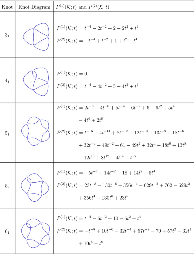
Table 6.1. P(1)(K;t) and P(2)(K;t) for 3
1 through 949 . . . 61
List of Figures
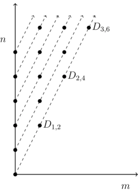
1.1. Summing along Diagonals . . . 3
2.1. Reidemeister Moves . . . 9
2.2. Conway Triple . . . 12
2.3. Elementary Braids . . . 13
3.1. Kauffman’s Skein Relation . . . 17
3.2. Associated Action for σi . . . 21
3.3. Associated Action for σ−i 1 . . . 22
3.4. Summing along Diagonals . . . 24
CHAPTER 1
Introduction
When studying knots or links, one often seeks to find the topological properties of
the objects being studied. A key question that one strives to answer when studying
knots is, “Are these two knots the same?” This includes seeing if a knot is really the
unknot. In the seemingly never-ending quest to answer these questions and others,
many different knot invariants have been discovered and explored.
Let K be a knot in S3. The Alexander polynomial ∆K(t) is a well understood
knot invariant that has a topological interpretation. In Chapter 2 we will provide
an overview of the Alexander polynomial. Further information about ∆K(t) can
be found in numerous texts including [16]. Another knot polynomial came onto
the scene in 1984 with the work of Vaughn Jones [13]. The Jones polynomial is a
polynomial knot invariant that seems similar to the Alexander polynomial in many
ways but is actually a totally different beast. In fact, the Jones polynomial is more
powerful than the Alexander polynomial, but it is defined purely combinatorially and
lacks any obvious topological interpretation within classical topology. Thus it was
particularly exciting when a non-rigorous path integral topological interpretation was
suggested by Witten in [27]. He suggested that the Jones polynomial is an infinite
dimensional integral over all SU(2) connections over S3 with a certain weight. The
colored Jones polynomial, Vα(K;q), is a generalized version of the Jones polynomial.
We will describe a way of calculating the colored Jones polynomial as a quantum
Melvin and Morton conjectured a relationship between the Jones and Alexander
polynomials in [18]. This conjecture was proven by Bar-Natan and Garoufalidis in
[4]. Rozansky extended the result further in [24].
Associate an (α+ 1)-dimensional Uq(sl(2))-module to a fixed knot, K ⊂ S3. Let
Jα(K;q) denote the colored Jones polynomial ofKnormalized so that it is
multiplica-tive under disjoint unions and
(1.0.1) Jα(unknot;q) =
qα/2−q−α/2 q1/2−q−1/2.
We will consider the reduced colored Jones polynomial defined as
(1.0.2) Vα(K;q) =
Jα(K;q)
Jα(unknot;q)
.
We have the following theorem due to Rozansky.
Theorem 1.0.1. Let K ⊂S3 be a knot. We have the following expansion for the
colored Jones polynomial in powers of h=q−1:
(1.0.3) Vα(K;q) = X
n≥0
hn X
0≤m≤n
Dm,n(K)(αh)2m !
such that the coefficients Dm,n+2m have the following property:
(1.0.4) X
m≥0
Dm,n+2m(K)(αh)2m =
P(n)(K;qα) ∆2Kn+1(qα/2−q−α/2),
where ∆K is the Alexander-Conway polynomial normalized so that ∆unknot = 1 and
P(n)(K;qα)∈
Z[qα, q−α] are invariants of the knot.
In this theorem, we sum along the diagonals in Figure 1.1.
Our work involves efficiently calculating these invariants,P(n)(K;qα), in the hopes
of gaining a wealth of experimental data from which we can infer some topological
properties. As will be described in Chapter 3, the Jones polynomial can be calculated
as a quantum trace. The calculation of Vα(K;q) is based on representation theory of
m n
D1,2
D2,4
D3,6
Figure 1.1. Summing along Diagonals
E, F, andH with relations
(1.0.5) [H, E] = 2E, [H, F] =−2F, and [E, F] = q
H −q−H
q−q−1
where q ∈ C. Let Wα denote an (α+ 1)-dimensional irreducible Uq(sl(2))-module.
There is an important Uq(sl(2))-intertwiner
(1.0.6) Rˇ :Wα⊗Wα →Wα⊗Wα
that satisfies the braid relations given in Section 2.4. This means there exists a
homomorphism
(1.0.7) f :Bn→EndUq(sl(2))(Wα⊗n)
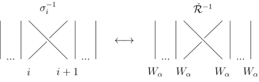
where Bn is the braid group on n generators, such that f(σi) = ˇRi where σi is an
elementary braid consisting of a single positive crossing of the ith strand over the
(i+ 1)st strand and
If a knot K is presented as a circular closure of a braid β ∈ Bn, then the Jones
polynomial is the “quantum trace”
(1.0.9) Vα(K;q) =qfrTrWα⊗n(QHf(β))
where QH = (qH/2)⊗n and qfr is a framing factor given by the Formula (3.4.1).
Im-portantly, one can compute only a partial trace. Namely, for a linear transformation
A:W⊗n
α →W
⊗n
α define
(1.0.10) Tr(1) :Wα →Wα
as a trace of A taken over all Wα factors except the first one. The partial quantum
trace of f(β) with a framing factor is proportional to the identity with the coefficient
being the reduced Jones polynomial Vα(K;q), i.e.
(1.0.11) qfrTr(1)
Wα⊗n(Q (1)
H f(β)) =Vα(K;q)1Wα
where Q(1)H =1⊗(qH/2)⊗(n−1).
Let us recall the more familiar classical case ofsl(2) before proceeding to the case
of Uq(sl(2)). The generators E,F, and H of sl(2) satisfy the relations
(1.0.12) [H, E] = 2E, [H, F] =−2F, and [E, F] =H.
In this case, we have a family of homomorphisms ˜fα : sl(2) → C[z, ∂z] where α ∈ C
and C[z, ∂z] is the Heisenberg algebra. Its action on the generators is
(1.0.13) f˜α(E) = z, f˜α(H) = α+ 2z∂z, and ˜fα(F) = −α∂z−z∂z2.
By deforming ˜f, we get a family of algebra homomorphisms fα : Uq(sl(2)) →
C[z, ∂z]. Before we describe the action of the homomorphisms on the generators of
Uq(sl(2)), let us define a function g(q, t, x)∈Z[t][[h, x]] as
(1.0.14) g(q, t, x) = −(q
x−q−x)(t qx−1/2−t−1q−x+1/2)
Let a=αh, so that α= a h and q
α =ea. Then the action of the family of
homomor-phisms on the standard generators E,H, and F is:
(1.0.15) fα(E) = z, fα(H) = α+ 2z∂z, and fα(F) = g(q, qα, z∂z + 1).
The Heisenberg algebra acts naturally on the polynomial algebra C[z], so the
homomorphism fα turnsC[z] into a Uq(sl(2))-module which we will denote by Cα[z].
Ifαis a positive integer, thenCα[z] has a submodulefWα generated overC[z] byzα+1.
That is, it is generated by {zα+1, zα+2, ...}over
C. The quotient module
(1.0.16) Wα=Cα[z]/Wfα
is the (α+1)-dimensional irreducible representation ofUq(sl(2)) generated by 1, z, z2, ..., zα
overC. The action of theUq(sl(2)) generators are given by the equations in (1.0.13).
Since the universalR-matrix ofUq(sl(2)) is given in terms of the generatorsE,F, and
H as in Equation (3.3.4), the action of ˇR, theR-matrix composed with permutation,
is determined by substituting the action of the generators into Equation (3.3.4).
For a knotK, it was shown in [24] that sinceWα is a quotientCα[z]/Wfα, one can
replace the factors Wα in the partial trace (1.0.11) by Cα[z]:
(1.0.17) qfrTr(1)(Cα[z])⊗nQ (1)
H f(β) =Vα(K;q)1Cα[z].
In order to produce the expansion in Theorem 1.0.1 and following [24], we study
the limit of Equation (1.0.17) when q → 1 and qα is constant. Let h = log(q) and
t=qα =ea. Then we can cast
(1.0.18) Rˇ :C[z1, z2]→C[z1, z2]
in the form
(1.0.19) Rˇ =Q(z1, z2, ∂z1, ∂z2) 1 +
∞
X
i=1
whereRi(z1, z2, w1, w2) is a polynomial of its arguments for eachiandRi(z1, z2, ∂z1, ∂z2)
is normal ordered while
(1.0.20) Q(z1, z2, ∂z1, ∂z2) = exp −z1∂z1 +tz2∂z1 +tz1∂z2 −t 2z
2∂z2
is a C[z1, z2]-algebra homomorphism, that is, Qacts on C[z1, z2] by a linear
transfor-mation on the generators z1 and z2. As a result f(β) has a similar form. Suppose
β ∈ Bn. Let z denote z1, z2, ..., zn and similarly let ∂z denote ∂z1, ∂z2, ..., ∂zn. Then
we can write
(1.0.21) f(β) = Qβ(z, ∂z) 1 +
∞
X
i=1
hiBi,β(z, ∂z) !
where Qβ(z, ∂z) is a C[z]-algebra homomorphism whose action on z1, z2, ..., zn
coin-cides with the Burau representation of β while Bi,β(z, ∂z) is a normal ordered
poly-nomial for each i. Recall the special relationship between the Burau representation
and the Alexander polynomial. The Alexander polynomial of a knot presented as a
braid closure can be computed as a determinant of the Burau representation of the
braid. Further details can be found in Section 2.5.
When h→0 andqα is kept constant, we are left with only the algebra
homomor-phism, Qβ. A partial trace of an algebra homomorphism can be computed by the
generalized geometric series formula. Let ˜Qβ denote the restriction of the action of
Qβ to the subspace Cn of variablesz2, ..., zn. Then we can write
(1.0.22) Tr(1)
C[z]Qβ =
1
detCn(1−Q˜β)
.
Since ˜Qβ coincides with the Burau representation, Equation (1.0.22) is precisely the
reason the Alexander polynomial appears in the expansion in Theorem 1.0.1.
However, we are interested in the case when h is nonzero. Thus it remains to
take the trace of the second portion of (1.0.21). To do this, we will use methods
from quantum field theory. We should stress that we are using these methods on a
are typically performed on a space with infinitely many variables. Hence all of these
techniques are completely rigorous in our setting. Our techniques will be explained
in Chapters 4 and 5, but here is a brief summary. Suppose that Qβ in the geometric
sum formula (1.0.22) depends on an extra parameter, so Equation (1.0.22) becomes
(1.0.23) Tr(1)
C[z]Qβ() =
1 detCn(1−Q˜β)
.
For a positive integerk, take thek-th derivative over epsilon of both sides and evaluate
at = 0:
(1.0.24) Tr(1)
C[z]
dkQβ()
dk
=0
= d
k
dk
1 detCn(1−Q˜β)
!
=0
.
Although d
kQ β()
dk is no longer an algebra homomorphism, this formula still computes
its trace. Equation (1.0.24) is the simplest example of the quantum field theory
techniques that we will use to compute the trace of the expanded formula (1.0.21).
We have developed a program in Mathematica [12] to efficiently perform these
techniques in rigorous finite-dimensional cases. Our program takes in information
about the braid representation of a knot and then calculatesP(1)(K;qα) andP(2)(K;qα).
We are now able to calculate P(1)(K;qα) and P(2)(K;qα) for any knot, and we will
present these polynomials for all prime knots up to nine crossings in Chapter 6. Also
in Chapter 6, we discuss a conjecture about our polynomials for amphicheiral knots
from [23] and provide evidence to the validity of the conjecture. In Chapter 4 we
will expand theR-matrix ofUq(sl(2)) in powers ofhto prove Theorem 4.1.1. We will
also provide a similar expansion of ˇR−1. In Chapter 5 we will discuss our methods
of calculation including how to take the trace of ˆβ, the action associated to a braid
β. We provide a copy of our program in Appendix A. We begin in Chapters 2 and 3
CHAPTER 2
The Alexander Polynomial
In this chapter we begin by discussing some preliminary definitions of knot theory.
Then we present three different interpretations of the Alexander polynomial ∆K(t).
These three include a topological interpretation, a skein-relation definition, and a
relationship with the Burau representation of the knot presented as a braid closure.
The last of these will play a role in our own calculations, but the topological
inter-pretation is the one of most interest. One of the biggest strengths of the Alexander
polynomial versus the Jones polynomial is the fact that the Alexander polynomial has
a topological interpretation while the Jones polynomial lacks one in classical topology.
We proceed with the preliminaries.
2.1. Preliminaries
The study of knots began in 1867 when Lord Kelvin suggested that atoms were
knotted up bits of ether. Because of this theory, physicists were interested in
tabulat-ing all possible knots. The Scottish physicist Tait started studytabulat-ing when two knots
are the same and created a table of knots. The following preliminary definitions are
adapted from [16].
Definition 2.1.1. A link L of m components is a subset of S3, or of R3, that
consists ofmdisjoint, piecewise linear, simple closed curves. A link of one component
is a knot K.
One can envision taking a string, tangling it somehow, and then fusing the ends.
Definition 2.1.2. LinksL1 and L2 inS3 are equivalent if there is an orientation
preserving piecewise linear homeomorphism h:S3 →S3 such thath(L1) =L2.
Oftentimes instead of studying the knots or links themselves, we study their
pro-jections into the plane.
Definition 2.1.3. A link diagram, D, of a link,L, is a projection into the plane
that keeps crossing information.
Of course, when studying the projections of links into the plane, we must
under-stand when two of these projections represent the same link.
Definition 2.1.4. A Reidemeister move refers to one of three local moves on a
link diagram. Each move operates on a small region of the diagram and is one of
three types:
(1) Twist and untwist in either direction.
(2) Move one loop completely over another.
(3) Move a string completely over or under a crossing.
These moves can be seen in Figure 2.1
↔ ↔ ↔
Figure 2.1. Reidemeister Moves
Two link diagrams belonging to the same link, up to planar isotopy, can be related
by a sequence of the three Reidemeister moves. This fact was shown independently
by Reidemeister in 1926 [21] and by Alexander and Briggs in 1927 [3].
Once we understand what it means for two knots, or knot diagrams, to be
One way that we can try to answer this question is by discovering and calculating knot
invariants. In fact, a variety of topological properties of knots can be investigated by
studying knot invariants.
Definition 2.1.5. A knot invariant is a quantity (in a broad sense) defined for
each knot which is the same for equivalent knots.
Another one of the questions mathematicians seek to answer about knots is, “Is
this the unknot?” Currently we know that the Alexander polynomial doesn’t detect
unknottedness, meaning we have examples of non-trivial knots of 10 crossings for
which the Alexander polynomial is equal to 1. It is still an open question whether the
Jones polynomial can detect unknottedness. These questions about knots and knot
invariants are interesting. Many knot invariants have been discovered and studied,
and this process continues today.
2.2. A Topological Definition of the Alexander Polynomial
The Alexander polynomial is perhaps the most well-known invariant of knots. This
polynomial was discovered by Alexander in 1928 [2]. The Alexander polynomial of a
knot can be interpreted topologically using an infinite cyclic cover of the complement
of the knot. A convenient way to view and build this infinite cyclic cover is through
Seifert surfaces. In this section, we will define these ideas rigorously. A reference for
the following discussion is [16].
Definition 2.2.1. A Seifert surface for an oriented link L in S3 is a connected
compact surface contained in S3 that hasL as its oriented boundary.
Of course now that we have this definition, a reasonable question to ask is, “Does
every knot have an associated Seifert surface?” The answer is yes for any oriented
link thanks to the following theorem.
This theorem was first proven by Frankl and Pontrjagin in [11]. In 1935 Seifert
provided another proof which is constructive [25]. His proof provided a general
method of finding a Seifert surface of a knot which is called the Seifert algorithm.
However this construction is not unique.
Although a Seifert surface is not necessary to have an infinite cyclic cover, we can
use it to build an infinite cyclic cover of the knot complement. As described in [16],
let F be a Seifert surface of L and let N be a regular neighborhood of L. Define X
to be the closure of S3 −N. Now let Y be X-cut-along-F. This means that Y is
homeomorphic toX less the open neighborhood F ×(−1,1). We can build X∞, the
infinite cyclic cover, by stacking countably many copies of Y on top of each other.
X∞ has a natural homeomorphism t :X∞ →X∞ which moves up one stack/copy of Y from the current position.
Definition 2.2.3. The rth Alexander ideal of an oriented link L is the rth
ele-mentary ideal of the Z[t, t−1]-module H1(X∞;Z). The rth Alexander polynomial of L is the generator of the smallest principal ideal of Z[t, t−1] that contains the rth
Alexander ideal. The first Alexander polynomial is called the Alexander polynomial
and is written ∆K(t).
If we restrict ourselves to considering the Alexander polynomial of a knot K, we
have a very satisfying interpretation of ∆K(t) as a characteristic polynomial presented
in [16].
Theorem 2.2.4. Let K be a knot in S3 and let t : X∞ → X∞ be the (covering)
translation of X∞ (the infinite cyclic cover of the exterior of K). Then H1(X∞;Q)is
a finite-dimensional vector space over the field Q. The characteristic polynomial of
the linear map t? :H1(X∞;Q)→H1(X∞;Q) is, up to multiplication by a unit, equal
Through this set up of the Alexander polynomial and the proceeding theorem, one
can see that the polynomial has its basis in topology. There are other descriptions of
the Alexander polynomial that are not topological in nature.
2.3. A Skein Relation Definition of the Alexander Polynomial
In 1970 Conway introduced his polynomial which satisfies certain skein relations
[9]. In fact, Alexander had shown that his polynomial satisfied the same relations.
This result was presented in the miscellaneous section of Alexander’s paper and was
thus not thoroughly investigated for some time. The Conway polynomial and the
Alexander polynomial are related by a simple formula and oftentimes the
polyno-mial knot invariant is simply called the Alexander-Conway polynopolyno-mial. The Conway
polynomial is defined in the following way.
Definition2.3.1. For oriented linksL, theConway polynomial ∇L(z)∈Z[z, z−1]
is defined by
(1) ∇unknot(z) = 1,
(2) whenever three oriented linksL+, L−,andL0 are the same except in a
neigh-borhood of a point where they are as shown in Figure 2.2, then
(2.3.1) ∇L+(z)− ∇L−(z) =z∇L0(z).
L+ L− L0
Figure 2.2. Conway Triple
The triple in Figure 2.2 is known as the Conway triple.
The Alexander polynomial is related to the Conway polynomial as follows:
for ∆L(t) normalized to satisfy the relation
(2.3.3) ∆L+(t)−∆L−(t) = (t
1/2 −t−1/2)∆ L0(t).
Oftentimes this is the method used to calculate the Alexander polynomial, but it lacks
the satisfying topological basis of the previous definition of the Alexander polynomial.
2.4. Presenting Knots as Braid Closures
In order to discuss the third interpretation of the Alexander polynomial, we must
pause here and discuss braids. Any braid is made up of elementary braids.
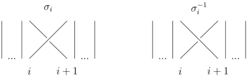
Definition 2.4.1. An elementary braid σi is a braid in which the only crossing
is the ith-strand crossing over the (i+ 1)st-strand. The inverse of σi, denoted σ−i 1, is
the braid consisting of only the crossing in which the (i+ 1)st-strand crosses over the
ith-strand.
σi
...
i i+ 1 ...
σ−i 1
...
i i+ 1 ...
Figure 2.3. Elementary Braids
The braid group on n-strands, Bn, is made up of elementary braids with certain
relations.
Definition2.4.2. Thebraid group onnstrands, denoted Bn, is generated by the
braids σi for i= 1, ..., n−1 subject to the relations
(2.4.1)
σiσi+1σi =σi+1σiσi+1 for 1≤i≤n−2
Then naturally, abraid is an element of Bn for somen ≥1.
The closure of a braidβ, denoted ¯β, is created by connecting corresponding ends
in pairs. We are talking about braids because there is a clear relationship between
braids and knots. We have the following theorem proven by Alexander in 1923 [1].
Theorem 2.4.3. Every knot can be presented as the closure of a braid.
Note that this theorem says nothing about the uniqueness of the braid
represen-tation of the knot, so we must ask when two different braid closures give rise to the
same knot. This question was answered by Markov in [17]. There are two actions on
a braid, called Markov moves, that we consider. The first is conjugation.
Definition 2.4.4. Given two braids α and β in Bn, a type 1 Markov move, also
called conjugation, takesαβ 7→βα.
We have another Markov move that is called a stabilization move.
Definition 2.4.5. Given a braid β ∈ Bn, a type 2 Markov move, also called a
stabilization move, takes β 7→βσn∈Bn+1 orβ 7→βσn−1 ∈Bn+1.
We can use these moves to determine when two braids will give rise to the same
knot. The following theorem is due to Markov [17].
Theorem 2.4.6. Given two braids α ∈ Bm and β ∈ Bn, we have that α¯ is
equivalent to β¯ if and only if β can be obtained from α through a finite sequence of
Markov moves.
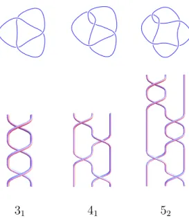
We conclude this section with a table that shows braid representations for the
some non-trivial knots. The knot diagrams in this table are from Knot Info [8] while
31 41 52
Table 2.1: Braid Representation of Some Knots
2.5. The Alexander Polynomial by the Burau Representation
There is yet another characterization of the Alexander polynomial using the
re-duced Burau representation of the braid group. The following definition of the rere-duced
Burau representation and Theorem 2.5.2 are presented in [5].
Definition 2.5.1. Let K be the closure of braid on n-strands, β. Let σi be the
elementary positive braid in which the ith strand crosses over the (i+ 1)st strand.
Then the reduced Burau representation associated to σi for i = 2, ..., n−1 is the
(n−1)×(n−1) matrix of the form
(2.5.1)
Ii−2
1 0 0
t −t 1
0 0 1
In−i−2
where Ir denotes the r×r identity matrix. When i = 1, we have a block matrix in
the upper left corner of the (n−1)×(n−1) matrix of the form:
(2.5.2)
−t 1
0 1
and the identity elsewhere. The reduced Burau matrix, B, associated to β is the
matrix product of the matrices associated to the sequence of elementary braids inβ.
Through the reduced Burau representation, we get the following theorem
concern-ing the Alexander polynomial. This theorem is presented in [5] as a modification of
a theorem of Burau from [7].
Theorem 2.5.2. For the Alexander polynomial, ∆K(t), and the reduced Burau
matrix, B, we have the following relationship
(2.5.3) ∆K(t) = det(B −I)
1 +t+. . .+tn−1.
Putting together the information in this section and the discussion from the
intro-duction, we can now understand why the Alexander polynomial appears in Theorem
1.0.1. Since the action ofQβ in the expansion off(β) coincides with the Burau
repre-sentation and taking the trace of such an expression introduces a factor of det(1−Q˜β),
CHAPTER 3
The Jones Polynomial as the Quantum Trace of a Braid
3.1. The Bracket Polynomial
The next knot invariant of interest is the Jones polynomial which can also be
defined using a skein relation. A reference for the following discussion is [14]. Often
we will be considering framed links.
Definition 3.1.1. A link L provided with a non-singular normal vector field is
said to be framed. Two vector fields on L that are homotopic in the class of
non-singular normal vector fields determine the same framing.
To compute the Jones polynomial using a skein class of diagrams, we must make
the following definitions.
Definition 3.1.2. Fix a nonzero complex number q. Let E(q) be the complex
vector space generated by all link diagrams quotiented by
(1) ambient isotopy in the plane;
(2) the relation D∪O =−(q+q−1)D, where D is an arbitrary link and O is a
simple closed curve bounding a disk in the complement of D;
(3) the identity in Figure 3.1 which is calledKauffman’s skein relation.
E(q) is a skein class of diagrams.
=q−1/2 +q1/2
Thus given a link diagram, one can use these relations to resolve any crossing of
the diagram.
Definition 3.1.3. Every link diagram D represents an element of E(q) which
will be denoted byhDi(q) or sometimes justhDi. This is called theskein class of D.
For knot diagrams, this skein class makes sense due to the following theorem
presented in [14].
Theorem 3.1.4. The skein class of any link diagram is invariant under the
Rei-demeister moves.
We should note that introducing a positive or negative curl as in the first
Rei-demeister move introduces a factor of −q−3/2 or −q3/2 respectively. However this is
considered to be equivalent in the skein class.
Using Theorem 3.1.4, we can define the bracket polynomial of a link L. Present
L by a diagramDand chooseq ∈C so that q+q−1 6= 0. Then we have the following
definition.
Definition 3.1.5. The bracket polynomial of L is
(3.1.1) hLi(q) =−(q+q−1)−1hDi(q).
Note that the bracket polynomial does depend on the framing of the link L.
3.2. The Jones Polynomial
Using the bracket polynomial we can define the Jones polynomial, V(L;q), of an
oriented link L inR3. In fact, we can define the Jones polynomial using the diagram
D of L. The Jones polynomial is basically the bracket polynomial with a framing
correction and renormalization.
Definition 3.2.1. Let ω(D)∈Z be the sum of all signs over all crossing points
Once we have this definition, we have the following theorem stated in [14] about
computing the Jones polynomial of a link diagram.
Theorem 3.2.2. Let |D| denote the number of crossing points of D. Then the
Jones polynomial can be calculated from the diagram D as follows:
(3.2.1) V(L;q) = (−1)|D|+1q3ω(D)/2hDi(q) q+q−1.
While this is a reasonable way to define the Jones polynomial, it can seem overly
complicated. There is a characterization like that of Theorem 2.3.1 for the Jones
polynomial from [14]. Recall that the Conway Triple is the relation in Figure 2.2.
Theorem 3.2.3. There exists a unique function
(3.2.2) V :{non-empty oriented links in R3} →Z[q, q−1]
such that
(1) if L is isotopic to L0, then V(L) =V(L0) (2) V(unknot) = 1
(3) for any Conway triple
q−2V(L+)−q2V(L−) = (q−q−1)V(L0)
Furthermore, this unique function is the Jones polynomial.
As was discussed in the introduction, the Jones polynomial is more powerful
than the Alexander polynomial, but it lacks any obvious topological interpretation
in classical topology. Witten introduced a path integral topological interpretation
in [27]. The Jones polynomial is an infinite dimensional integral over all SU(2)
connections over S3 with a certain weight. We should note that if you compute this
integral with the help of perturbation theory, then you get an expansion of the Jones
polynomial in powers of (q−1) or log(q). In the next chapter, we will be expanding
3.3. The Quantum Group Uq(sl(2))
The colored Jones polynomial, Vα(K;q), is a generalized version of the Jones
polynomial. Here α denotes coloring by an (α + 1)-dimensional representation of
Uq(sl(2)). Note that V1(K;q) = V(K;q). The colored Jones polynomial can be
calculated usingR-matrices of quantum groups. Here we considerUq(sl(2)), the Hopf
algebra with generatorsE, F, and H satisfying:
(3.3.1) [H, E] = 2E, [H, F] =−2F, and [E, F] = q
H −q−H
q−q−1
with comultiplication given by:
(3.3.2)
∆(E) =E⊗qH + 1⊗E
∆(F) =F ⊗1 +q−H ⊗F
∆(H) =H⊗1 + 1⊗H
This is a natural definition for the comultiplication ofUq(sl(2)). For a Lie algebra
we usually have that
(3.3.3) ∆(x) =x⊗1 + 1⊗x,
so that the comultiplication respects the commutator of the Lie algebra. This is also
the case for our quantum group. The comultiplication is chosen in the above way so
that it respects the commutator. For example, [∆(H),∆(E)] = ∆([H, E]).
Uq(sl(2)) acts on tensor products, but because of the above definition of the
co-multiplication, permutation P : V ⊗W → W ⊗V which takes v ⊗w 7→ w⊗v is
not an Uq(sl(2)) intertwiner. However we do have many different intertwiners. We
consider a special one that satisfies the Yang-Baxter equation and the braid relation.
This intertwiner is called an R-matrix and is given as follows:
(3.3.4) R=q(H⊗H)/2 ∞
X
n=0
where
(3.3.5) Rn(h) =qn(n−1)/2(q−q−1)n([n]q!)−1 and [n]q =
qn−q−n q−q−1 .
A good reference for this is [15].
3.4. Calculating the Colored Jones Polynomial
As previously stated, one can calculate the colored Jones polynomial using this
R-matrix structure. This method was developed by Reshetikin and Turaev in [22].
First present the knot K as the closure of a braid β. Using Theorem 2.4.3, we know
that any knot can be presented as a braid closure. To any braid β of n-strands, one
can associate an action ˆβ onW⊗n
α whereWα is an (α+ 1)-dimensional representation
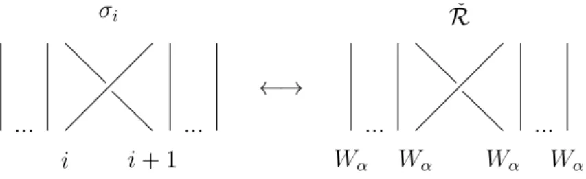
of Uq(sl(2)). To the elementary braid σi, we associate ˇR, the R-matrix composed
with permutation, acting on Wα⊗Wα at the ith and (i+ 1)st positions in Wα⊗n as in
Figure 3.2 and described thoroughly in the introduction.
σi
...
i i+ 1 ...
←→
ˇ
R
...
Wα Wα
...
Wα Wα
Figure 3.2. Associated Action for σi
We associate ˇR−1,R−1 composed with permutation, to the negative elementary braid
σi−1 as in Figure 3.3.
In this construction the action of braids commutes with the global action ofUq(sl(2)).
σi−1
...
i i+ 1 ...
←→
ˇ
R−1
...
Wα Wα
...
Wα Wα
Figure 3.3. Associated Action for σi−1
Theorem 3.4.1. Present a knot K as the closure of a braid β. Let βˆ denote
the representation of β acting on W⊗n
α . Then the colored Jones polynomial can be
calculated as the quantum trace of the braid, i.e.
Vα(K;q) =qfrTrWα⊗n(q
H/2)⊗nβ,ˆ
where (qH/2)⊗n denotes an operator that acts asqH/2 on each module W
α of Wα⊗n. fr is a framing correction:
(3.4.1) fr=−1/4(α2−1)e(β),
where e(β) equals the number of positive elementary braids minus the number of
neg-ative elementary braids in β.
3.5. The Melvin-Morton-Rozansky Expansion
In the 1990’s a relationship between the Jones and Alexander polynomials was
explored. Melvin and Morton made the following conjecture concerning the colored
Jones polynomial in [18].
Theorem 3.5.1. Let Vα(K) ∈ Q(q) be the “framing independent colored Jones
polynomial” of the knotK, i.e. the framing independent Reshetikhin-Turaev invariant
of K colored by the (α+ 1)-dimensional representation of sl(2). Let h be a formal
parameter and let q =eh. Then expanding V
α(K;eh) in powers of α and h,
Vα(K;eh) = X
j,m≥0
we have:
(1) “Above diagonal” coefficients vanish: ajm(K) = 0, if j > m.
(2) “On diagonal” coefficients give the inverse of the Alexander-Conway
polyno-mial:
(3.5.1) M M(K)(h)·∆K(q)(eh) = 1,
where ∆K(q) is the Alexander-Conway polynomial and M M is defined by
(3.5.2) M M(K)(h) =
∞
X
m=0
amm(K)hm.
Here we note that this conjecture was proven by Bar-Natan and Garoufalidis in
an equivalent form in [4]. This idea was studied further by Rozansky in [24]. Here
we switch to the set up and notation of [24]. Let K be a knot in S3. Associate an
α-dimensionalUq(sl(2))-module to the knot. LetVα(K;q) denote the reduced colored
Jones polynomial ofKnormalized so that it is multiplicative under disconnected sums
and Vα(unknot;q) = 1. In this set up, an equivalent statement of Theorem 3.5.1 is
as follows.
Theorem 3.5.2. Let K ⊂ S3 be a knot and h = q−1. We have the following
expansion for the colored Jones polynomial:
(3.5.3) Vα(K;q) = X
n≥0
hn X
0≤m≤n
Dm,n(K)α2m !
such that the coefficients Dm,n have the following properties:
(1) Dm,n(K) = 0 for m >
n 2, (2) X
m≥0
Dm,2m(K)a2m =
1 ∆K(t−t−1),
where a is a formal parameter, ∆K is the Alexander-Conway polynomial normalized
so that ∆unknot = 1, and t=eiπa.
Note that the second part of the theorem says to sum along the first diagonal in
In fact, there is another theorem which involves summing along other diagonals
which gives powers of the the Alexander polynomial in the denominator. This theorem
is due to Rozansky [24]. In this theorem, we sum along the other diagonals in
Figure 3.4.
Theorem 3.5.3. Let K ⊂ S3 be a knot and h = q−1. We have the following
expansion for the colored Jones polynomial:
(3.5.4) Vα(K;q) = X
n≥0
hn X
0≤m≤n
Dm,n(K)(αh)2m !
such that the coefficients Dm,n+2m have the following property:
(3.5.5) X
m≥0
Dm,n+2m(K)(αh)2m =
P(n)(K;qα/2−q−α/2)
∆2Kn+1(qα/2−q−α/2) ,
where ∆K is the Alexander-Conway polynomial normalized so that ∆unknot = 1and
P(n)(K;qα)∈Z[qα, q−α] are invariants of the knot.
m n
D1,2
D2,4
D3,6
Figure 3.4. Summing along Diagonals
In the next chapters, we will describe our methods of calculatingP(1)(K;qα) and
P(2)(K;qα) and then present these polynomials for all prime knots up to nine crossings.
An amphicheiral knot is one that is isotopic to its mirror image. The interesting
property is given as a conjecture by Rozansky in [23] stated by expanding in a new
parameter
(3.5.6) ˜h= (1 +h)1/2 −(1 +h)−1/2.
Expanding Vα(K;q) in ˜h, we have
(3.5.7) Vα(K;q) =
∞
X
n=0
˜
V(n)(K;qα/2−q−α/2)˜hn.
Then the conjecture is as follows:
Conjecture 3.5.4. For an amphicheiral knot K,
(3.5.8) V˜(2n−1)(K;qα/2−q−α/2) = 0
and
(3.5.9) V˜(2n)(K) = ˜
P(2n)(K;qα/2−q−α/2)
∆3Kn+1(qα/2−q−α/2)) .
for all n ≥1.
Note that this conjecture says two things of importance. The first is thatP(2n−1)(K;qα)
vanishes for all n ≥ 1 for amphicheiral knots. The second is that for n ≥ 1,
P(2n)(K;qα) is divisible by the powers of Alexander polynomial for amphicheiral knots.
When we present our results in Chapter 6, we will provide evidence to the validity of
this conjecture. We present the first two polynomials for all amphicheiral knots up
to ten crossing and will show that the polynomials have the properties in Conjecture
CHAPTER 4
Expansion of the
R
-matrix
4.1. The h-adic Hopf Algebra Uh(sl(2))
In this chapter we are concerned with expanding the universalR-matrix ofUq(sl(2))
in powers of h = log(q). First we discuss the generators of the Uh(sl(2)) themselves,
then we move on to further techniques. We will calculate an expansion of each term
in the R-matrix and then talk about how we can put the pieces together to get an
expression of the form
(4.1.1) ˇR=Q(z1, z2, ∂z1, ∂z2)(1+h R1(z1, z2, ∂z1, ∂z2)+h 2R
2(z1, z2, ∂z1, ∂z2)+O(h 3))
First we begin with a description ofUh(sl(2)).
Uh(sl(2)) is the h-adic Hopf algebra with generators E, F, and H satisfying:
(4.1.2) [H, E] = 2E, [H, F] =−2F, and [E, F] = e
hH−e−hH
eh−e−h
with comultiplication given by:
(4.1.3)
∆(E) = E⊗ehH+ 1⊗E
∆(F) = F ⊗1 +e−hH⊗F ∆(H) = H⊗1 + 1⊗H
The universal R-matrix is given by
(4.1.4) R=eh(H⊗H)/2 ∞
X
n=0
where
(4.1.5) Rn(h) =ehn(n+1)/2(1−e−2h)n([n]q!)−1 and [n]q =
ehn−e−hn eh −e−h .
Furthermore, R has an inverse given by
(4.1.6) R−1 =e−h(H⊗H)/2
∞
X
n=0
e−hnRn(h)((ehHE)n⊗(ehHF)n).
We denote the R-matrix composed with permutation by ˇR. Similarly, ˇR−1 denotes
the inverse R-matrix composed with permutation. For further discussion on this, see
[15] or [14].
For the remainder of the chapter, we aim to prove a theorem about the
expan-sion of the R-matrix. As discussed in the introduction, there is a family of algebra
homomorphisms fα :Uq(sl(2))7→C[z, ∂z] whereα ∈Cand C[z, ∂z] is the Heisenberg
algebra. Recall that its action on the standard generators E, H, and F is:
(4.1.7) fα(E) =z, fα(H) =α+ 2z∂z, and fα(F) =g(q, qα, z∂z+ 1),
for
(4.1.8) g(q, t, x) =−(q
x−q−x)(t qx−1/2−t−1q−x+1/2)
x(q−q−1)(q1/2−q−1/2) ∈Z[t][[h, x]].
We will provide a proof of the action offαonF in Proposition 4.2.1 using the
commu-tator relations on the generatorsE, H, andF. Using this family of homomorphisms,
we can state our main theorem. As in the introduction, the Heisenberg algebra acts
naturally on C[z], so fα turns C[z] into a Uq(sl(2))-module denoted Cα[z]. If fWα
denotes the submodule over Cα[z] generated by zα+1, then the quotient module
(4.1.9) Wα=Cα[z]/Wfα
is the (α+1)-dimensional irreducible representation ofUq(sl(2)) generated by 1, z, z2, ..., zα
with the action of E, F, and H given by Equation (4.1.7). Then the R-matrix acts
Theorem 4.1.1. Let t =qα and h= log(q). Then Rˇ of Uh(sl(2)) can be written
as
(4.1.10)
ˇ
R=Q(z1, z2, ∂z1, ∂z2)(1 +h R1(z1, z2, ∂z1, ∂z2) +h 2R
2(z1, z2, ∂z1, ∂z2) +O(h 3)),
with
(4.1.11) Q(z1, z2, ∂z1, ∂z2) = exp −z1∂z1 +tz2∂z1 +tz1∂z2 −t 2z
2∂z2
,
(4.1.12)
R1(z1, z2, ∂z1, ∂z2) =
−2t2− 1
t2 + 3
z12∂z22 +
2t− 2
t
z21∂z1∂z2
+
1 t −3t
z1z2∂z22 + 2z1z2∂z1∂z2,
and
(4.1.13)
R2(z1, z2, ∂z1, ∂z2) =
4t3− 16t
3 + 4 3t
z13∂z32+
−4t3+ 2
t3 + 10t−
8 t
z14∂z32∂z1
+
6t3− 1
t3 −11t+
6 t
z2z13∂ 4 z2 +
−4t2− 1
t2 + 5
z12∂z22
+ 4−4t2z13∂z2
2∂z1 +
2t2+ 2 t2 −4
z14∂z2
2∂ 2 z1 + 4t2 3 − 2 3t2 +
10 3
z2z12∂z32
+
9t2
2 + 1 2t2 −3
z22z12∂z4
2 +
−10t2− 4
t2 + 14
z2z13∂ 3 z2∂z1
+
2t4+ 1 2t4 −6t
2− 3
t2 +
13 2
z14∂z42 +
2t− 2
t
z21∂z2∂z1
+
2t− 2
t
z13∂z2∂ 2 z1 +
1 t −5t
z2z1∂z22 + 2 3t − 14t 3
z22z1∂z32
+
−2t− 2
t
z2z12∂ 2 z2∂z1 +
2 t −6t
z22z12∂z32∂z1 + 2z2z1∂z2∂z1
+
4t− 4
t
z2z13∂ 2 z2∂
2 z1 + 2z
2
2z1∂z22∂z1 + 2z2z 2 1∂z2∂
2 z1 + 2z
2 2z
2 1∂
2 z2∂
Our key technique will appear over and over in this chapter. For each piece of the
R-matrix, we will express it as a higher order term and an exponential of a bilinear
form in z1, z2, ∂z1 and ∂z2. When we say higher order term, we mean a term of the
form
(4.1.14) 1 +h P1(z1, z2, ∂z1, ∂z2) +h 2
P2(z1, z2, ∂z1, ∂z2) +O(h 3
).
For each portion of the R-matrix, we will have an exponential of a bilinear form in
z’s and ∂z’s and higher order terms. We will normal order each higher order term as
we go along. An expression is normal ordered if all partial derivatives appear to the
right of any multiplication by z. To complete our theorem, we will have to move a
higher order term through the exponential of a bilinear form. The mechanisms of this
moving will be discussed in Chapter 5, but it amounts to making linear substitutions
inz1,z2,∂z1, and∂z2.
4.2. The Generators E, F, and H
We want to use quantum groups to calculate the colored Jones polynomial of a
knot as in Chapter 3. However, we will do it in such a way that we will automatically
get the expansion in powers of h in Theorem 3.5.3. The idea is outlined as follows.
We will first represent the knot as a braid closure. Next we will look at the associated
action of ˆβ on W⊗n
α as before. As explained in the introduction and the previous
section, we consider Wα, which is the (α+ 1)-dimensional irreducible representation
ofUq(sl(2)) generated by 1, z, z2, ..., zα with the action ofE,F, andH as in Equation
(4.1.7). Before expounding on this forUq(sl(2)), let us recall the more familiar classical
case.
Consider sl(2) which has generators E, F, andH that satisfy the relations
In this case, we have a family of homomorphisms ˜fα : sl(2) → C[z, ∂z]. We want
to define its action on the generators E, F, and H. It is reasonable to make the
following choices for E and H:
(4.2.2) f˜α(E) =z and f˜α(H) = α+ 2z∂z.
Then
(4.2.3) [ ˜fα(H),f˜α(E)] = [α+ 2z∂z, z] = 2z= 2 ˜fα(E)
as required. From here we can figure out what ˜fα(F) should be, using the relation
[E, F] = H. Let us make an informed guess that ˜fα(F) = b∂z +c∂z2. After solving
for the coefficients, we find that b=−α and c=−z, so
(4.2.4) f˜α(F) = −α∂z −z∂z2.
With this choice of ˜fα(F), we have that [ ˜fα(H),f˜α(F)] =−2 ˜fα(F), and [ ˜fα(E),f˜α(F)] =
˜
fα(H) as required.
We wish to do a similar process with the generators of Uq(sl(2)). Now we will let
q=eh, a=αh, and t=qα =ea.
Proposition 4.2.1. Let t=qα and h = log(q). If
(4.2.5) fα(E) =z and fα(H) =α+ 2z∂z,
then
(4.2.6)
fα(F) = −
t−t−1 2h ∂z−
t+t−1 2 z∂
2 z −
t−t−1 12 h(4z
2∂3
z + 6z∂z2−∂z)
− t+t
−1
12 h
2
Proof. We can expand F in powers of h by considering
(4.2.7)
F En|0i=
n−1 X
k=0
En−k−1[F, E]Ek|0i
=
n−1 X
k=0
En−k−1
−q
H −q−H
q−q−1
Ek|0i
=− 1
q−q−1 n−1 X
k=0
(tq2k−t−1q−2k)En−1|0i
=− 1
q−q−1
t q
2n−1
q−1 −t −1 q
−2n−1
q−1−1
En−1|0i
=−(q
n−q−n)(t qn−1/2−t−1q−n+1/2)
(q−q−1)(q1/2−q−1/2) E n−1|0i
for t=qα =ea.
Once we have this expression, we can expand
(4.2.8) −(q
n−q−n)(t qn−1/2−t−1q−n+1/2)
(q−q−1)(q1/2−q−1/2)
in powers of h. Doing so, we arrive at the following
(4.2.9)
F En|0i=
−t−t
−1
2h n+
t+t−1
2 n(n−1)−
t−t−1
12 h(4n(n−1)(n−2) + 6n(n−1)−n)
−t+t
−1
12 h
2
(2n(n−1)(n−2)(n−3) + 8n(n−1)(n−2) + 3n(n−1)) +O(h3)
En−1|0i
Now we can write fα(F) in powers of h as follows:
(4.2.10)
fα(F) =−
t−t−1 2h ∂z−
t+t−1 2 z∂
2 z −
t−t−1 12 h(4z
2∂3 z + 6z∂
2 z −∂z)
−t+t
−1
12 h
2(2z3∂4
z + 8z2∂z3+ 3z∂z2) +O(h3).
4.3. Expansion of Rn(h)
We are now ready to work on expanding the pieces of the R-matrix of Uh(sl(2)).
First we concern ourselves with
(4.3.1) Rn(h) =qn(n+1)/2(1−q−2)n([n]q!)−1.
Lemma 4.3.1. We can expand Rn(h)in powers of h= log(q) and get the first few
terms as follows:
(4.3.2)
Rn(h) =qn(n+1)/2(1−q−2)n([n]q!)−1
=ehn(n+1)/2(1−e−2h)n([n]q!)−1
= (2h)
n
n!
1 + h
2n(n−1) + h2
72(9n(n−1)(n−2)(n−3) + 32n(n−1)(n−2) + 12n)
+O(h3)
Proof. In order to calculate the expansion, we take the natural log of some of
the pieces in (4.3.2), work on each piece, then exponentiate to return to what we
wish. First we have that
(4.3.3) ln(ehn(n+1)/2) = h
1
2n(n+ 1)
+O(h2).
Next we expand
(4.3.4) n(ln(1−e−2h) = n
ln(2) + ln(h)−h+h
2
6 − h4
180 +O(h
6)
.
Now we work on an expansion of [n]q!. Recall that
(4.3.5) [n]q =
qn−q−n
q−q−1 =
ehn−e−hn
eh−e−h .
Consider
(4.3.6) e
hk−e−hk
eh−e−h =k
1 +h2 k
2−1
6 +h
4 3k
4 −10k2+ 7
360 +O(h
6)
Taking the natural log yields
(4.3.7) ln
ehk−e−hk eh−e−h
= ln(k) +h2 k
2−1
6 +h
4 k 4−1
180 +O(h
6).
In order to calculate [n]q!, we sum (4.3.7) with k running from 1 to n. Doing so we
obtain (4.3.8) n X k=1 ln
ehk−e−hk
eh−e−h
= ln(n!) +h2 n(2n
2+ 3n−5)
36 −h
4 n(6n4+ 15n3+ 10n2−31)
5400 .
Finally, we exponentiate (4.3.3) + (4.3.4)−(4.3.8) and obtain that
(4.3.9)
Rn(h) =
(2h)n
n!
1 + h
2n(n−1)
+h
2
72(9n(n−1)(n−2)(n−3) + 32n(n−1)(n−2) + 12n) +O(h
3)
.
4.4. Expansion of En⊗Fn
Now that we have expanded Rn(h), we must tackle En⊗Fn. First we use the
result of Lemma 4.3.9 to write
(4.4.1) ∞
X
n=0
Rn(h)En⊗Fn=
∞
X
n=0
(2h)n
n! E
n⊗Fn !
1 + h
2(2hE⊗F)
2+ h2
2 9(2hE ⊗F)
4
+32(2hE⊗F)3+ 12((2hE⊗F)+O(h3)
= exp(2hE ⊗F)
1 + h
2(2hE⊗F)
2+h2
2 9(2hE⊗F)
4
+32(2hE⊗F)3+ 12((2hE⊗F)+O(h3) .
Before proceeding further, we pause here and expand
(4.4.2)
1 + h
2(2hE⊗F)
2
+h
2
2 9(2hE⊗F)
4
Lemma 4.4.1. Let T =t−t−1 and S =t+t−1. The expansion in powers of h of Formula (4.4.2) is
(4.4.3) 1 +h s1(z1, z2, ∂z1, ∂z2) +h 2s
2(z1, z2, ∂z1, ∂z2) +O(h 3),
where
(4.4.4) s1(z1, z2, ∂z1, ∂z2) =
1 2T
2z2 1∂z22
and
(4.4.5) s2(z1, z2, ∂z1, ∂z2) =
1 2ST z
2 1∂
2
z2+ST z 2
1z2∂z32+
1 8T
4z4 1∂
4 z2−
4 9T
3z3 1∂
3 z2−
1
6T z1∂z2.
Proof. There is not much to do here. We simply expand (4.4.2) and normal
order the terms based on the commutator relation
(4.4.6) [∂zi, zj] =δij.
Doing so yields (4.4.3).
4.5. Expansion of exp(2hE⊗F)
We are now ready to work on expanding each part of Equation (4.4.1). For each
of these pieces, we will have an exponential of a bilinear form and a higher order part
which consists of normal ordered polynomials inz1, z2, ∂z1 and ∂z2. First we consider
exp(2hE ⊗F). We wish to express this as
(4.5.1)
exp(2hE⊗F) = Q2(z1, z2, ∂z1, ∂z2) 1 +hq1(z1, z2, ∂z1, ∂z2) +h 2
q2(z1, z2, ∂z1, ∂z2) +O(h 3
).
Proposition 4.5.1. We can expand exp(2hE ⊗F) in powers of h and get that
(4.5.2)
exp(2hE⊗F) = exp(−T z1∂z2) 1 +h q1(z1, z2, ∂z1, ∂z2) +h 2
q2(z1, z2, ∂z1, ∂z2) +O(h 3
with
(4.5.3) Q2(z1, z2, ∂z1, ∂z2) = exp(−(t−t
−1)z 1∂z2),
(4.5.4) q1(z1, z2, ∂z1, ∂z2) =−
1 2ST z
2 1∂
2
z2 −Sz1z2∂ 2 z2,
and
(4.5.5)
q2(z1, z2, ∂z1, ∂z2) =
1
6T z1∂z2 −
1 2T
2z2 1∂
2 z2
2S2T
3 −
2T3
9
z13∂z32 +1 8S
2T2z4 1∂
4 z2
+
S2−2T 2
3
z12z2∂z32 +
1 2S
2
T z13z2∂z42 +
1 2S
2
z21z22∂z42
−T z1z2∂z22 −
2 3T z1z
2 2∂
3 z2.
Proof. First recall that
(4.5.6) fα(E1) = z1
and
(4.5.7)
fα(F2) = −
t−t−1
2h ∂z2 −
t+t−1
2 z2∂
2 z2 −
t−t−1
12 h(4z
2 2∂
3
z2 + 6z2∂ 2
z2 −∂z2)
− t+t
−1
12 h
2(2z3
2∂z42 + 8z 2
2∂z32 + 3z2∂ 2
z2) +O(h 3).
Thus we can write
(4.5.8)
2hE1⊗F2 =−(t−t−1)z1∂z2−
t+t−1
h z1z2∂
2 z2−
t−t−1
6 h
2z 1(4z22∂
3
z2+6z2∂ 2
z2−∂z2)+O(h 3).
Before finding the higher order part, let us consider the exponential term. We must get
a normal ordered expression of exp(−(t−t−1)z1∂z2), denoted : exp(−(t−t
−1)z
1∂z2) : .
Because z1 and ∂z2 commute, there is nothing to be done here. We have that
(4.5.9) exp(−(t−t−1)z1∂z2) = : exp(−(t−t
−1)z
Thus we have
(4.5.10) Q2(z1, z2, ∂z1, ∂z2) = exp(−(t−t
−1)z 1∂z2).
For convenience, we set T = t−t−1 and S = t+t−1. Proceeding to the higher
order term, we consider
(4.5.11) U(s) =e−Ases(A+hB)
where
(4.5.12) A=−T z1∂z2
and
(4.5.13) B =−h(Sz1z2∂z22)−h 2
2T 3 z1z
2 2∂
3
z2 +T z1z2∂ 2 z2 −
T 6z1∂z2
.
Since we are looking for an expansion in h, we write
(4.5.14) U(s) = 1 +hU1(s) +h2U2(s) +O(h3)
Differentiating both (4.5.11) and (4.5.14) gives us that
(4.5.15) U10(s) = e−s adAB,
where adA on B is the usual adjoint action [A, B]. Thus
(4.5.16)
U1(s) = Z s
0
e−τ adAdτ
B
= 1−e −s adA
adA
B.
We can expand this in powers ofadA and conclude that at the order ofh we have the
following
(4.5.17) B+ 1
2[A, B] + 1
6[A,[A, B]]− 1
which can be written as a normal ordered operator in terms of z1, z2, ∂z1, and ∂z2
which gives the desired
(4.5.18) P1(z1, z2, ∂z1, ∂z2) = −
1 2ST z
2 1∂
2
z2 −Sz1z2∂ 2 z2.
Proceeding in a similar fashion, we see that
(4.5.19) U20(s) =e−s adA1U
1(s) = e−s adA1
1−e−s adA2
adA2
(B, B).
Here we have introduced the notationAi to mean that this copy of A acts on theith
copy of B in the above expression. Again, we integrate and find that
(4.5.20) U2(s) =
1 adA2
1−e−s adA1
adA1
− 1−e
−s(adA1+adA2)
adA1 +adA2
(B, B).
Again expanding the above expression in adAi and performing the adjoint action on
the appropriate copies of B, we get the following,
(4.5.21) 1 2B
2−1
3[A, B]·B+ 1
8[A,[A, B]]·B− 1
6B·[A, B]− 1
8[A, B][A, B] + 1
24B·[A,[A, B]].
Once we compute the commutators and normal order the expression, we get the
desired
(4.5.22)
P2(z1, z2, ∂z1, ∂z2) =
1
6T z1∂z2 −
1 2T
2
z12∂z22
2S2T
3 −
2T3
9
z13∂z32 +1 8S
2
T2z14∂z42
+
S2− 2T 2
3
z12z2∂z32 +
1 2S
2T z3
1z2∂z42 +
1 2S
2z2 1z
2 2∂
4 z2
−T z1z2∂z22 −
2 3T z1z
2 2∂
3 z2.
4.6. Expansion of exp(h(H⊗H)/2)
Next we turn our attention to exp(h(H⊗H)/2). As before, we wish to write this
Proposition 4.6.1. For exp(h(H⊗H)/2) we can write
(4.6.1)
eh(H⊗H)/2 =ea2/2hQ1(z1, z2, ∂z1, ∂z2) 1 +h p1(z1, z2, ∂z1, ∂z2) +h 2p
2(z1, z2, ∂z1, ∂z2) +O(h 3)
,
with
(4.6.2) Q1(z1, z2, ∂z1, ∂z2) = exp((t−1)(z1∂z1 +z2∂z2)),
(4.6.3) p1(z1, z2, ∂z1, ∂z2) = 2z1z2∂z1∂z2,
and
(4.6.4) p2(z1, z2, ∂z1, ∂z2) = 2z1z2∂z1∂z2 +z 2
1z2∂z21∂z2 + 2z1z 2 2∂z1∂
2 z2 + 2z
2 1z22∂z21∂
2 z2
Proof. Finding the expression in Equation (4.6.1) is a simple matter of
expand-ing and normal orderexpand-ing. The calculation is as follows
(4.6.5)
exp(h(H⊗H)/2) = exp
h 2
a
h+ 2z1∂z1
a
h + 2z2∂z2
= exp(a2/2h) exp(a(z1∂z1 +z2∂z2)) exp(2hz1z2∂z1∂z2).
Once we expand the third exponential in powers of h and normal order the
coeffi-cients, we arrive at Equations (4.6.3) and (4.6.4). Now we turn our attention to the
exponential. For the moment, we will ignore exp(a2/2h) as it will be taken care of in
our final calculations as a framing factor. Now we must normal order the exponential.
Normal ordering we get that
(4.6.6) exp(a(z1∂z1 +z2∂z2) = : exp((e a−
1)(z1∂z1 +z2∂z2)) : .
Thus we conclude that
(4.6.7) Q1(z1, z2, ∂z1, ∂z2) = exp((t−1)(z1∂z1 +z2∂z2)).
In order to complete the proof of Theorem 4.1.1, we must understand how to
compose the exponential terms and how to move a normal ordered operator through
an exponential of a bilinear form. For a discussion on the mechanisms of composing
and moving through exponentials of bilinear forms, see the next chapter. Now that
we have the required expansions, we complete the proof of Theorem 4.1.1 here.
4.7. Proof of Theorem 4.1.1
Proof. Using the previous propositions and lemmas, we have expanded the
pieces of theR-matrix into exponential and higher order terms. Let us take an
inven-tory of what we have. For ease of notation we will often writep1 forp1(z1, z2, ∂z1, ∂z2),
Q1 for Q1(z1, z2, ∂z1, ∂z2), and so on. From Proposition 4.5.1, we have written
(4.7.1) exp(2hE⊗F) =Q2 1 +h q1+h2q2+O(h3)
.
From Lemma 4.4.1, we have written Equation (4.4.2) as
(4.7.2) 1 +h s1+h2s2+O(h3).
Furthermore, using Proposition 4.6.1, we have expanded
(4.7.3) eh(H⊗H)/2 =Q1 1 +h p1+h2p2+O(h3)
.
Now we must appropriately combine these pieces and normal order the resulting
higher order term. First let us combine (4.7.1) and (4.7.2) since all we need to do is
multiply
(4.7.4) 1 +h q1+h2q2 +O(h3)
· 1 +h s1+h2s2+O(h3)
and normal order the results. Doing so gives us
(4.7.5) N(z1, z2, ∂z1, ∂z2) = 1 +h n1 +h 2n
where
(4.7.6) n1(z1, z2, ∂z1, ∂z2) =
1 t2 −1
z12∂z22 +
−t− 1
t
z2z1∂z22
and
(4.7.7)
n2(z1, z2, ∂z1, ∂z2) =
2t3
3 − 2
3t3 + 2t−
2 t
z13∂z3
2 +
t− 1
t3
z2z31∂ 4 z2
+
1− 1
t2
z12∂z22 +
4t2 3 −
2 3t2 +
10 3
z2z12∂z32
+
t2
2 + 1 2t2 + 1
z22z12∂z4
2 +
1 2t4 −
1 t2 +
1 2
z14∂z4
2
+
1 t −t
z2z1∂z22 + 2 3t − 2t 3
z22z1∂z32.
In order to combine the higher order pieces from (4.7.3) and (4.7.5), we must move
(4.7.8) 1 +h p1+h2p2+O(h3)
through the exponential Q2 of (4.7.1). Using the results of Proposition 5.2.1, this
amounts to making linear substitutions on z1, z2, ∂z1,and ∂z2 as in equations (5.2.5)
and (5.2.9). These substitutions are
(4.7.9) z1 7→z1, z2 7→z2+ (t−t−1)z1, ∂z1 7→∂z1 −(t−t
−1)∂
z2, and ∂z2 7→∂z2.
Once we do this moving through and normal order the resulting higher order term,
we arrive at
(4.7.10) 1 +hp˜1+h2p˜2+O(h3),
where
(4.7.11)
˜
p1(z1, z2, ∂z1, ∂z2) =
−2t2− 2
t2 + 4
z21∂z22 +
2t−2
t
z12∂z2∂z1
+
2 t −2t
and
(4.7.12)
˜
p2(z1, z2, ∂z1, ∂z2) =
−4t3+ 4
t3 + 12t−
12 t
z41∂z32∂z1 +
4t3− 4
t3 −12t+
12 t
z2z13∂ 4 z2
−2t2z2z21∂z32 + 2t 2z2
2z21∂z42 +
−2t2− 2
t2 + 4
z12∂z22
+
−2t2− 2
t2 + 4
z31∂z22∂z1 +
2t2+ 2 t2 −4
z41∂z22∂z21
+
−8t2− 8
t2 + 16
z2z31∂ 3 z2∂z1 −
2z2z12∂z32
t2 +
2z2 2z12∂z42
t2
+
2t4+ 2 t4 −8t
2− 8
t2 + 12
z14∂z42 +
2t− 2
t
z12∂z2∂z1
+
2t− 2
t
z31∂z2∂ 2 z1 +
2 t −2t
z2z1∂z22 +
2 t −2t
z22z1∂z32
+
4 t −4t
z22z21∂z32∂z1 +
4t−4
t
z2z31∂ 2 z2∂
2
z1 + 4z2z 2 1∂
3 z2
−4z22z12∂z4
2 + 2z2z1∂z2∂z1 + 2z 2
2z1∂z22∂z1 + 2z2z 2 1∂z2∂
2 z1
+ 2z22z21∂z22∂z21.
Only one more step remains to get the higher order term associated to ˇR. We must
multiply and normal order
(4.7.13) 1 +hp˜1+h2p˜2+O(h3)
· 1 +h n1+h2n2+O(h3)
.
Doing so yields
(4.7.14) 1 +h R1(z1, z2, ∂z1, ∂z2) +h 2R
2(z1, z2, ∂z1, ∂z2) +O(h 3),
with R1 and R2 given by Equations (4.1.12) and (4.1.13) respectively.
To conclude, we must prove that Q(z1, z2, ∂z1, ∂z2) is given by Formula (4.1.11).
To establish this, we will show that the action on z1 and z2 of the composition ofQ1,