ESSAYS ON MONETARY POLICY IN OPEN ECONOMIES
Ezequiel R. Cabezon
A dissertation submitted to the faculty of the University of North Carolina at Chapel Hill in partial fulfillment of the requirements for the degree of Doctor of Philosophy in the Department of Economics.
Chapel Hill 2013
Approved by:
Richard Froyen
Anusha Chari
Neville Francis
William Parke
ABSTRACT
EZEQUIEL R. CABEZON: ESSAYS ON MONETARY POLICY IN OPEN ECONOMIES.
(Under the direction of Richard Froyen.)
This dissertation studies whether monetary policy has short run effects on output in emerging
economies and characterizes the mechanisms of transmission of the monetary policy. Specifically it
focuses on the real effects of the monetary policy in Brazil, where policymakers introduced structural
reforms earlier than other emerging economies. Chapter I identifies the effects of monetary policy
in Brazil using a vector autoregressive model. It finds that monetary policy has short run effects
on output and nearly none on prices. This contrasts with the policy wisdom that monetary policy
in EMEs can only affect prices. Chapter II, studies the interest rate channel of monetary policy in
Brazil. It finds that surprise changes in the monetary policy interest rates have larger effects on the
market interest rate during expansions than in recessions. This is attributed to the larger expected
duration of expansion over recesions. Chapter III, uses a Dynamic Stochastic General Equilibrium
model to study the effects of monetary policy when firms borrow to finance their working capital
in an open economy. This issue is crucial in cases like Brazil where working capital credit explains
half of the firms’ borrowing and it quadrupled in the last 15 years. A monetary policy tightening
has two effects: i) It discourages consumption (the traditional demand channel) and ii) It increases
the production cost (known as the working capital channel). The final effect on inflation is unclear
as these effects work in opposite directions. The model concludes that in an open economy where
there is working capital borrowing, the aggregate demand channel dominates the working capital
ACKNOWLEDGEMENTS
I am grateful to Professor Richard Froyen for his continuous guidance, encouragement and support
at every stage of this dissertation. I am also indebted to Pau Rabanal and the committee members
TABLE OF CONTENTS
LIST OF TABLES . . . ix
LIST OF FIGURES . . . x
1 Chapter 1. Does Monetary Policy Have Real Effects? The Brazilian Case . . 1
1.1 Introduction . . . 1
1.2 VAR Methodology and Literature Review . . . 2
1.2.1 VAR Methodology . . . 2
1.2.2 VAR’s Evidence . . . 4
1.2.3 Evidence for Brazil . . . 5
1.3 Estimation and Results . . . 6
1.3.1 Estimation . . . 6
1.3.2 Robustness . . . 8
1.4 Industry Effects of Monetary Policy . . . 15
1.5 Effects of Monetary Policy during 1994-99 and 2000-12 . . . 17
1.6 Conclusions . . . 19
2 Chapter 2. Monetary Policy and Market Interest Rates in Brazil . . . 20
2.1 Introduction . . . 20
2.2 Previous Studies . . . 22
2.2.1 Theoretical Perspective . . . 22
2.2.2 Empirical Perspective . . . 23
2.3.1 Data . . . 25
2.3.2 Estimating the Effect of Anticipated and Unanticipated Monetary Shocks . . 25
2.3.3 Effects of Monetary Shocks During Recessions and Expansions . . . 27
2.4 Conclusions . . . 32
3 Chapter 3. Working Capital, Financial Frictions and Monetary Policy . . . 33
3.1 Introduction . . . 33
3.2 Literature Review . . . 36
3.3 The Model . . . 38
3.3.1 Households . . . 40
3.3.2 Firms . . . 42
3.4 Cost Channel in Closed and Open Economies . . . 53
3.4.1 Parameters in the Simulations . . . 53
3.4.2 Results . . . 54
3.4.3 Robustness and Model Evaluation . . . 58
3.5 The Cost Channel in an Open Economy with Imported Inputs . . . 59
3.5.1 Domestic Producer . . . 60
3.5.2 Balance of payments . . . 61
3.5.3 Exogenous variables . . . 62
3.6 Summarizing the Models . . . 64
3.7 Conclusion . . . 65
A Appendix - Chapter 1 . . . 67
A.1 Specification . . . 67
A.2 Summary Literature VARs . . . 68
A.3 Quarterly Estimations . . . 70
A.4 Does Monetary Policy Affect the Retail Borrowing Rates? . . . 72
A.6 Stationarity Tests . . . 76
B Appendix - Chapter 2 . . . 77
B.1 Summary Statistics . . . 77
B.2 Log-likelihood Optimization . . . 78
B.3 Estimations: Sample 2004-2013 . . . 79
C Appendix - Chapter 3 . . . 82
C.1 Log-Linear Model - Section 3.3 . . . 82
C.2 Working Capital Without Financial Frictions . . . 85
C.3 Sensitivity Analysis . . . 86
C.3.1 Openness . . . 86
C.3.2 Pass-through . . . 87
C.3.3 Indexation . . . 88
C.3.4 Monetary Rule Interest Rate Smoothing . . . 89
C.3.5 Alternative Monetary Shocks . . . 90
C.3.6 Accuracy of the Model . . . 91
LIST OF TABLES
1.1 Summary: Cumulative Impulse Response Functions . . . 14
2.1 Estimation - 2003-2013 . . . 26
2.2 Subsample Estimation - 2003-2013 . . . 28
2.3 State Dependent Estimation - 2003-2013 . . . 31
3.1 Percent of Working Capital Financed with Credit . . . 34
3.2 Simulation Parameters . . . 54
A.1 VARs in Closed Economies . . . 68
A.2 VARs in Open Economies . . . 69
A.3 Lag structure test . . . 75
A.4 Monthly Frequency - Unit Root Tests . . . 76
A.5 Quarterly Frequency - Unit Root Tests . . . 76
B.1 Main Interest Rates . . . 77
B.2 Estimation - 2004-2013 . . . 80
LIST OF FIGURES
1.1 Recursive Specification . . . 8
1.2 Structural Specification I . . . 10
1.3 Structural Specification II . . . 11
1.4 Recursive Specification - Quarterly Estimation . . . 12
1.5 Recursive Specification - Lag Sensitivity . . . 12
1.6 Recursive Specification - Sensitivity to Output and Price Measures . . . 14
1.7 Industry Effects - Recursive Specification . . . 17
1.8 Recursive Specification - 1994-1999 and 2000-2012 . . . 18
2.1 Sample 2003-2013 - 3-Month Interest Rate . . . 32
3.1 Lending to Firms in Brazil . . . 35
3.2 Assets Flow . . . 38
3.3 Goods Flow . . . 39
3.4 Goods Flow: Extended Model . . . 60
3.5 Summary - Cumulative Deviations from Steady State . . . 65
A.1 Structural I - Quarterly Estimation . . . 70
A.2 Structural II - Quarterly Estimation . . . 70
A.3 Recursive Specification - Quarterly - Sensitivity to Lags and Output . . . 71
A.4 Recursive Specification - Quarterly - Sensitivity to Price Measures . . . 71
A.5 Industry Effects - Quarterly - Recursive Specification . . . 72
A.6 Response of Retail Interest Rates . . . 74
B.1 Monetary Policy Rate . . . 77
B.2 Log-likelihood . . . 78
C.2 Sensitivity to Openness Degree . . . 86
C.3 Sensitivity to Pass-through in Exchange Rate . . . 87
C.4 Sensitivity to Indexation . . . 88
C.5 Sensitivity to Smoothing of Interest Rate in the Monetary Rule . . . 89
C.6 Effect of Consecutive Shocks . . . 90
Chapter 1
Does Monetary Policy Have Real Effects? The Brazilian Case
1.1 Introduction
This chapter’s goal is to measure the effect of monetary policy in Brazil for the period 2000 to
2012. Specifically, it intends to document if monetary policy has a real effect on output. There is
no clear consensus about the size of these effects across different countries. In addition the evidence
about the effects of monetary policy across different industries is limited.
This question can be translated in theoretical terms as determining if a New Keynesian (NK)
model or a Real Business Cycle (RBC) better fits the Brazilian economy movements. A New
Keynesian model predicts that after a monetary policy tightening output will decrease as a result
of price stickiness and prices will reduce with less intensity. Meanwhile, a Real Business Cycle
model predicts no real effect on output and negative effects on prices. In fact, NK predicts stronger
effects on output and weaker effects on prices, while the RBC predicts stronger effects on prices
and weaker effects on output.
In empirical terms several authors measured these effects for Brazil, but most of the literature
focused on sample periods before the mid 1990s. Since 1999, Brazil has introduced important
structural reforms. In particular, in 1999 it established an inflation targeting framework and
a flexible exchange rate. Since then the economy has stabilized significantly. Now there is a
reasonable number of observations available to explore the real effects of monetary policy in this
An accurate measure of the sign and size of the response of output to monetary policy shocks is
crucial to set monetary policy size and its timing. In theoretical terms, determining whether a NK
model or a RBC model is a better representation of the economy, has important implications in the
setup of the monetary policy rules. If the RBC model is the correct model (meaning that it better
represents the economy) the optimal monetary policy rule must be an strict inflation targeting,
while if the correct model is the NK model, then there is room for discussion about setting a
flexible inflation targeting scheme.
Using a Vector Autorregression (VAR) and a wide range of specifications, this chapter found
that output responds significantly to monetary policy shocks and that prices have a weak response.
Specifically it found that after a 25 basis points unanticipated increase in the monetary policy rate
industrial production decreases around 3.0% and prices increases 0.27% after 12 months.
This chapter is divided into 6 sections. Section 1.1 provides the background. Section 1.2 reviews
the VAR methodology and previous literature. Section 1.3 analyzes the effect of monetary policy
on aggregate output. Section 1.4 studies the industry effects of monetary policy (durable,
non-durable, intermediate inputs and capital goods). Section 1.5 compares how output and prices
responses under the inflation targeting and flexible exchange rate regime (2000-2012) differ from
the responses observed under the fixed exchange rate regime (1994-1998). Section 1.6 sets the
conclusions.
1.2 VAR Methodology and Literature Review
This section provides a review of VARs methodology and summarizes the evidence documented
in previous research.
1.2.1 VAR Methodology
The goal of a VAR is to identify how innovations in monetary policy instruments affect other
variables such as output, prices, etc. The estimation of VAR’s impulse responses implies using
exogenous innovations1. Sims (1980) introduced VARs to measure the idea that unanticipated
movements in money aggregates have real effects on output. Sims’s contribution was pointing
that these unanticipated movements or surprises can be measured as the errors from the VAR’s
equations. In particular the errors of the equation that measures the monetary policy stance can
be interpreted as exogenous monetary policy shocks.
A VAR is specified in general as:
A0Zt=A(L)Zt+F(L)Xt+Bet (1.1)
Equation 1.1 describes a structural relationship among “n” endogenous variables in the vector
Zt (of dimension nx1). A0 describes the contemporaneous relationship among variables, A(L) is a
polynomial including “L” lags. Xt is a vector of “m” exogenous variables (e.g.: constant, trend,
or known variables in period t), F(L) is a polynomial with “L” lags, et are structural innovations
of the system, andB describes the contemporaneous relations among these structural innovations.
By re-writing Equation 1.1 it is possible to obtain Equation 1.2, which is known as the reduced
form of the VAR.
C(L) =A−01A(L), D(L) =A−01F(L), ut=A−01Bet
Zt=C(L)Zt+D(L)Xt+ut (1.2)
The key point in a VAR estimation is the identification conditions of structural and reduced
innovations. In other words the set up of matricesA0 and B is what matters. This is because they
relateutandetbyut=A−01Bet. There are two main ways to identify these matrices: i) a recursive
identification or ii) a structural identification.
A recursive identification is when A0 is a triangular matrix and B is an identity matrix (this
is known as Choleski specification)2. This assumes that structural innovations are independent
1
VARs focus on deviations of the systematic monetary policy. This is not trivial as these are the only situations where the effect of exogenous monetary policy shocks on other economic variables can be measured.
2
between each other and that the reduced innovations are related by the lower triangular set up. ut
is a vector of unobservable innovations (reduced form innovations) that can be estimated directly
from Equation 1.2. The coefficients fromA0 can be estimated from Equation 1.3.
E(utu0t) =E(A0−1ete0t[A−01]
0) (1.3)
A structural identification (or Structural VAR) imposes restrictions based on prior theory. A
first approach is to set zero or arbitrary constrains on the contemporaneous relationships (that is
on the coefficients of A0 and B) and a second approach is to impose constrains on the cumulative
response functions. The second is denoted as identification by long run constrains.
1.2.2 VAR’s Evidence Evidence for the U.S.
Literature assessing the effects of monetary policy for the U.S. concludes that after a monetary
tightening output and prices respond negatively. The second conclusion is that prices response
is weak. Sims (1980), using a recursive identification, found that after a monetary tightening
industrial production falls and prices have non-significant increment. Bernanke and Blinder (1992)
estimated a recursive VAR where they found similar results but they used the interest rate as
the monetary policy stance. Christiano, Eichenbaum and Evans (1999) reached the same results
(i.e.: a significant effect on output and a non-significant effect on prices) using a wide range of
data specifications. A summary of the main VARs estimations for U.S. is included in Table A.1.,
Appendix A.2.
Evidence for Open Economies
Estimations of VARs in open economies provide less clear results in terms of output (output is
not always significant and it is small when it is significant) and in most cases show price puzzles3
3
as well as exchange rate puzzles4. The main contributions can be summarized by5:
i Sims (1992), using a recursive identification, documents that output responds negatively to
interest rate innovations for the G-5 countries. He reported price and exchange rate puzzles
and argued that the introduction of a proxy variable for anticipated inflation can reduce both
puzzles.
ii Kim and Roubini (2000) avoided price and exchange rate puzzles by introducing a structural
VAR, which constrains contemporaneous relationships. They allowed monetary policy to
re-spond contemporaneously to the price of oil and the exchange rate. The idea of including oil
prices was to offset supply shocks. They concluded that after an unexpected increase in the
in-terest rate, there is: 1) a reduction of monetary aggregates, output and prices and 2) a nominal
exchange rate appreciation.
1.2.3 Evidence for Brazil
VAR estimations that measure the effects of monetary policy for Brazil either focus on periods
before inflation targeting framework was established or rest on unrealistic assumptions. The main
related studies to the current paper are:
i Rabanal and Schwartz (2001) estimated a VAR for the period 1995-2000 and found that output
responds negatively and significantly to changes in the interest rate. They also documented
a price puzzle. The issue with this paper is that the period 1995-2000 involves two different
foreign exchange policy regimes6. This may be introducing distortions in his estimations.
ii Minella (2003) studied the period 1994-2000 and found similar results to Rabanal and Schwartz
but no effect on prices. His estimation suffers from the same problem as Rabanal and Schwartz.
It is argued that inflation targeting frameworks allow agents to anticipate monetary policy and
therefore reduce the effects of monetary shocks. For this reason it is relevant to check if the
estimation is still accurate.
4
An exchange rate puzzle refers to a situation where after an increase in interest rate, an increase in nominal exchange rate is observed.
5
iii Cat˜ao and Pagan (2010) analyzed the credit channel in Brazil with a VAR for the inflation
targeting period but their specification rests on a structural model where the financial sector
plays a key role in financial intermediation. It is difficult to support this assumption considering
the distortions in the Brazilian financial sector. Public banks and the national development
bank (BNDES) play a crucial role in the financial sector providing credit to target sectors and
at targeted rates7. Their estimation found that after an increase in the nominal interest rate
output and price fall. The estimations I develop below find similar results, but without modeling
the financial sector.
1.3 Estimation and Results
1.3.1 Estimation
In this subsection a recursive VAR is estimated and it is shown that under several specifications
output responds negatively to innovations in the monetary policy rate. The effects on prices are
not significant in most cases. Estimation was done using monthly data (January 2000 until
De-cember 2012) because the larger number of observations allows for more accurate estimations. The
estimated VAR is set as:
Zt=C1Zt−1+C2Zt−2+DV,0XV,t+DV,1XV,t−1+D2,VXV,t−2+DC,0XC,t+ut (1.4)
The selection of the variables is consistent with Kim and Roubini (2000).
Zt =
IPt CP It Rt Mt N ERt
0
(1.5)
XV,t =
F Ft P Comt
0
(1.6)
XC,t =
T rendt Constant
0
(1.7)
7
IPt: log of industrial production index, seasonally adjusted.
CP It: log of consumer price index, seasonally adjusted.
Rt: Monetary policy target rate (SELIC) - monthly average.
M1t: log of nominal M1 - monthly average, seasonally adjusted.
N ERt: log of nominal exchange rate $BR / US$ - monthly average.
F Ft: Fed Funds target rate - monthly average.
P Comt: log of the commodity price index BCB.
The estimation was done in log levels except for interest rates as in most of the literature. A
trend term was added in the regression, in order to turn the variables stationary and estimate the
VAR using OLS. Although unit root test performed suggest that the series follow a first difference
stationary process (See Appendix A.6), this chapter uses log levels and explicit trend for two
reasons: i) This chapter follows most of the literature, which works in log-levels (Christiano et al.
(1999)8) and ii) It has been shown that the power of several unit root test is low, meaning that
they frequently fail to reject the unit root hypothesis when it is actually false (Maddala and In-Moo
(1999)). The benchmark estimation uses a Choleski identification consistent with Christiano et al.
(1999).
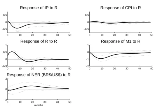
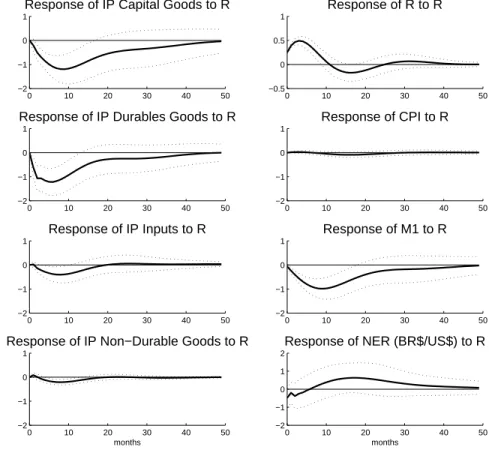
The impulse response functions and the 90% confidence bands of the benchmark estimation are
shown in Figure 1.1. The specification points out that after a 25 basis points unexpected increase
in the monetary policy rate we observe:
i A significant and temporary contraction in industrial production.
ii A contraction of prices after a year, but not significant.
iii A significant and temporary contraction of M1.
iv No exchange rate puzzle.
8
Figure 1.1: Recursive Specification
Impulse response function in percent points and the 90% confidence interval
0 10 20 30 40 50
−0.5 0 0.5
Response of IP to R
0 10 20 30 40 50
−0.5 0 0.5
Response of CPI to R
0 10 20 30 40 50
−0.5 0 0.5 1
Response of R to R
0 10 20 30 40 50
−2 −1 0 1
Response of M1 to R
0 10 20 30 40 50
−2 0 2
Response of NER (BR$/US$) to R
months
1.3.2 Robustness
VAR estimations are subject to several issues and for this reason sometimes they are not
consid-ered a reliable tool. The main issues to be taken into account are: i) Impulse response estimations
are highly sensitive to the identification assumptions9, ii) Estimations are sensitive to the unit of
frequency and the sample period, iii) Estimations are sensitive to lag specifications, and iv) There
are doubts about the appropriate variable to measure monetary stance.
This chapter tries to answer part of these issues by doing robustness checks. The first issue is
partially addressed by using structural identifications. The second issue is partially tested using
quarterly data to perform the estimations10. The third issue is answered considering different lag
9
Recursive VAR appear to identify the effects of monetary policy without a structural model, but actually they are still implying a structural model as they assumeA0 to be lower triangular matrix to identify endogenous monetary
policy actions from exogenous monetary policy actions. In most literature specification is ad-hoc except for Sims and Zha (1998) which is the only paper that tries to provide a theoretical microfundamented model for the identification used.
10
structures, and the fourth issue does not represent a problem since the background provides clear
information that the monetary policy instrument is the nominal interest rate.
Structural Identifications
This chapter will perform two structural identifications. The first will include the idea of the
interest rate only responding to inflation. The second identification will incorporate the idea that
price shocks affect output.
The first structural VAR was estimated using identification constrains similar to Kim and Roubini
(2000). The main difference is that the interest rate responds to current inflation in order to reflect
the inflation target. This identification scheme will be referred to as “Structural I” from now on.
∗ 0 0 0 0
∗ ∗ 0 0 0
0 ∗ ∗ 0 0
∗ ∗ ∗ ∗ 0
∗ ∗ ∗ ∗ ∗
| {z }
A0 uIP,t
uCP I,t
uR,t
uM1,t
uN ER,t
=
1 0 0 0 0
0 1 0 0 0
0 0 1 0 0
0 0 0 1 0
0 0 0 0 1
| {z }
B eIP,t
eCP I,t
eR,t
eM1,t
eN ER,t
The first line of the matrixA0 states that the structural innovation on output (IP) only depends
contemporaneously with itself. The idea is that within a period output only responds to
productiv-ity shocks. The second line states the idea that output and inflation are related through a Phillips
curve. The exchange rate is excluded from the price equation, reflecting that the pass-through from
the exchange rate to prices is not instantaneous. The third line states the monetary rule where
the central bank of Brazil responds to prices11. Note that the exchange rate is excluded from the
monetary policy reaction function because the monetary framework sets inflation as the only goal.
The fourth line is the money demand which depends contemporaneously on the interest rate, the
level of prices and the activity. Finally the exchange rate is contemporaneously related with all
variables as it is a forward looking variable.
11The assumption of the central bank responding to current prices is accurate considering that Brazil has measures
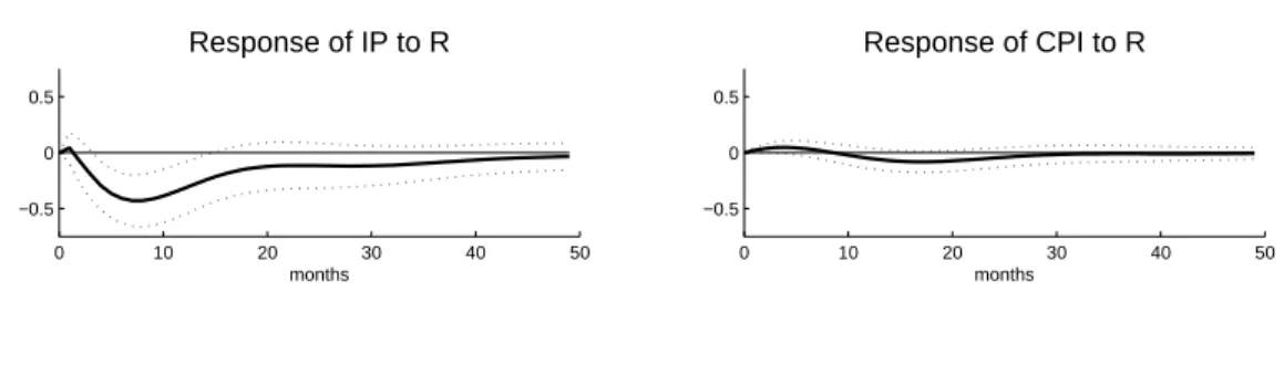
The impulse response of the “Structural I” estimation is shown in Figure 1.2. They present
similar results as the benchmark case. There is a small price puzzle as it is observed in many
papers and the reason is that the central bank responds in anticipation to the inflation.
Figure 1.2: Structural Specification I
Impulse response function in percent points and the 90% confidence interval
0 10 20 30 40 50
−0.5 0 0.5
Response of IP to R
0 10 20 30 40 50
−0.5 0 0.5
Response of CPI to R
0 10 20 30 40 50
−0.5 0 0.5 1
Response of R to R
0 10 20 30 40 50
−2 −1 0 1
Response of M1 to R
0 10 20 30 40 50
−1 0 1 2
Response of NER (BR$/US$) to R
months
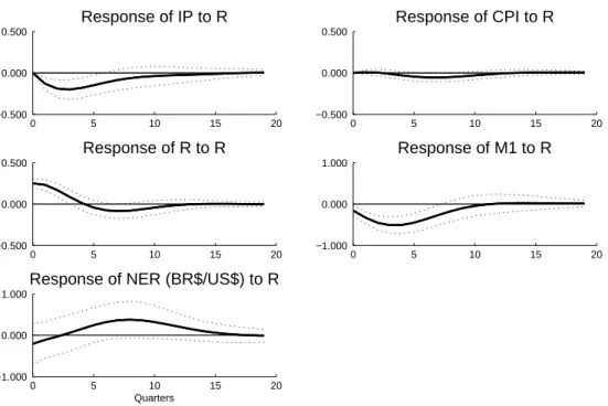
The second structural identification scheme allows prices to be independent contemporaneously,
while prices and output are related by the Phillips curve. Basically the order between IP and CPI
was exchanged compared with the benchmark case. The matrix below shows the identification
changes. This identification scheme will be denoted “Structural II” from now on.
∗ ∗ 0 0 0
0 ∗ 0 0 0
∗ ∗ ∗ 0 0
∗ ∗ ∗ ∗ 0
∗ ∗ ∗ ∗ ∗
| {z }
A0 uIP,t
uCP I,t
uR,t
uM1,t
uN ER,t
=
1 0 0 0 0
0 1 0 0 0
0 0 1 0 0
0 0 0 1 0
0 0 0 0 1
| {z }
B eIP,t
eCP I,t
eR,t
eM1,t
eN ER,t
The impulse response of the “Structural II” estimations are shown in Figure 1.3. They describe
similar results as the benchmark case: significant and short term negative effects on IP and negative
but non-significant effects on prices.
Figure 1.3: Structural Specification II
Impulse response function in percent points and the 90% confidence interval
0 10 20 30 40 50 −0.5
0 0.5
Response of IP to R
months
0 10 20 30 40 50 −0.5
0 0.5
Response of CPI to R
months
Frequency Sensitivity
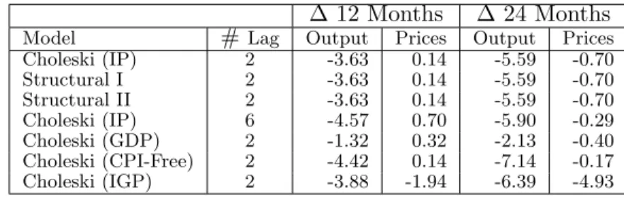
The second robustness issue analyzed is the sensitivity of impulse response functions to the data
frequency. In order to address this issue the estimations are done using quarterly data and the same
identification assumptions as in the monthly frequency estimations. The results (shown in Figure
1.4) are very similar to the monthly results. Output responds significantly and prices respond but
non significantly. Appendix A.3 analyzes all the robustness cases at quarterly frequency.
Lag Sensitivity
The third robustness tests are related with the lag specification. The argument for checking lag
sensitivity rests on the idea that there may be some omitted variables. Although the test for lag
extension indicates that the correct lag extension is two lags (see Appendix A.5), in this section
we estimate a 6 lags VAR to check the sensitivity. The reason for choosing six lags is that it is
widely accepted that monetary policy takes at least two quarters to affect the economy. In Figure
1.5 Panel A and B show the impulse response of a VAR including 6 lags. The results are similar to
the results of the benchmark case (Figure 1.1): strong effects on output and weak effect on prices.
Sensitivity to Output and Price Measures
Figure 1.4: Recursive Specification - Quarterly Estimation
Impulse response function in percent points and the 90% confidence interval
0 5 10 15 20
−0.500 0.000 0.500
Response of IP to R
0 5 10 15 20
−0.500 0.000 0.500
Response of CPI to R
0 5 10 15 20
−0.500 0.000 0.500
Response of R to R
0 5 10 15 20
−1.000 0.000 1.000
Response of M1 to R
0 5 10 15 20
−1.000 0.000 1.000
Response of NER (BR$/US$) to R
Quarters
Figure 1.5: Recursive Specification - Lag Sensitivity
Impulse response function in percent points and the 90% confidence interval
0 10 20 30 40 50 −1
−0.5 0 0.5 1
A: Response of IP to R
0 10 20 30 40 50 −1
−0.5 0 0.5 1
B: Response of CPI to R
0 10 20 30 40 50 −1
−0.5 0 0.5 1
C: Response of GDP to R
months
0 10 20 30 40 50 −1
−0.5 0 0.5 1
D: Response of CPI to R
months
Activity12, which approximates GDP better than IP. This index shows a smaller variance as a result
of the effect of the services. The results of this estimation are shown in Figure 1.5 Panels C and D.
These results are similar to the benchmark case. Output responds negatively in the short run and
prices fall after a year. The main difference with the benchmark case is that the output response is
half of the response observed in the benchmark case. One reason for the weaker effects on output
is that the Index of Economic Activity includes information from the farming sector and services.
The low response of farming is attributed to the high sensitivity of the sector to weather conditions.
In the services industry, the low response to interest rates is explained by the high persistence in
services such as government services and education.
The fifth robustness check is related to the price measures. Most VARs estimations are subject
to price puzzles. In general there are two main explanations for these puzzles. The first one is that
there is an omitted variable problem (meaning that expected prices are not included in the VAR).
The second explanation is that a large component of CPI corresponds to regulated prices, which
may not respond. Most of the papers that find a negative effect of interest rate on prices use broad
measures of prices such as GDP deflator. This measure responds more to economic conditions
because it includes wholesale prices, which are more flexible. For these reasons we re-estimate the
benchmark VAR and its impulse response functions by replacing CPI by two different measures
of prices: 1) CPI-Free Prices (non-regulated goods and services) and 2) Index of General Prices13,
which approximates the GDP deflator.
In Figure 1.6 Panels A and B show the impulse response functions of IP and prices for the case
where CPI is replaced by CPI-Free Prices (non-regulated). The idea is to exclude the prices which
are not allowed to respond to market incentives. Finally Panel C and D show the results for the
estimation using the Index of General Prices (IGP). The results do not change significantly from
the benchmark. Industrial production responds strongly and prices show mixed results. While
12
The index is available since 2003. For January 1999 until December 2002, the index was estimated using the Chow and Lin (1971) method. This method estimates monthly GDP from quarterly GDP data using monthly information from industrial production, real retail sales and basic construction inputs. For the period where the Economic Index Activity and the estimation are available the correlation is 99.78.
con-CPI-Free Prices register no response, IGP responds negatively and significantly.
Figure 1.6: Recursive Specification - Sensitivity to Output and Price Measures
Impulse response function in percent points and the 90% confidence interval
0 10 20 30 40 50
−1 −0.5 0 0.5 1
A: Response of IP to R
0 10 20 30 40 50
−1 −0.5 0 0.5 1
B: Response of CPI−FREE to R
0 10 20 30 40 50
−1 −0.5 0 0.5 1
C: Response of IP to R
months
0 10 20 30 40 50
−1 −0.5 0 0.5 1
D: Response of IGP to R
months
Summarizing the Responses
This section concludes that monetary policy has strong effects on output and weak effects on CPI
prices. Considering the cumulative impulse response functions (Table 1.1) the chapter concludes
that an unanticipated 25 basis point increase in monetary policy rates, reduces IP 3.63 percent and
increases CPI 0.14 percent after 12 months. CPI only responds negative after 24 months at -0.70
percent. The impulse response function also shows that the same change in the monetary policy
rate reduces the deflator (IPG) -1.94 percent after 12 months.
Table 1.1: Summary: Cumulative Impulse Response Functions
∆ 12 Months ∆ 24 Months
1.4 Industry Effects of Monetary Policy
This section documents the response of output in different industries to monetary shocks. Studies
such as Peersman and Smets (2005) and Dedola and Lippi (2005) document industry effects for the
Euro Area. They concluded that industries related to durable consumption goods and capital goods
are more sensitive to monetary shocks. There are two main reasons for heterogeneous effects of
monetary policy across industries: i) certain goods’ demands depend significantly on the borrowing
cost as these goods are purchased with credit; ii) certain industries depend more on bank financing
than others to finance their working capital. Therefore changes in the interest rate will affect the
demand and the borrowing cost of the firms asymmetrically across industries.
This section considers only four different groups (Capital Goods, Durable Goods, Non-Durable
Goods and Intermediate Inputs) to keep the number of parameters to be estimated at a low number.
The first two groups’ demands depend on financing conditions. In particular Brazil has shown an
important growth in the credit lines for vehicles financing and personal loans (mainly allocated
to Durable Goods). The microeconomics behind this is that a monetary shock that increases the
cost of borrowing affects negatively the demand of Durable Goods, such as cars, refrigerators, TV,
etc. The Capital Goods’ demand depends on the interest rate because the present value of the
investment projects depends on the interest rate. A monetary shock that increases the interest rate
significantly reduces the demand for Capital Goods. Finally certain goods’ demand depends less
on the interest rate. The demand of Non-Durable Goods due to its nature is almost independent of
the interest rates (e.g. food and beverages) while the Intermediate Inputs depend highly on foreign
markets (e.g. basics chemical inputs, steel and rubber).
The estimations assume that shocks to different industries are independent in order to avoid
arbitrary assumptions about the interrelation among industries.
Zt=
IPtKG IPtDCG IPtN DCG IPtIIG CP It Rt Mt N ERt
0
IPtKG: log of Capital Goods IP index, S.A.
IPDCG
t : log of Durable Consumption Goods IP index, S.A.
IPtN DCG: log of Non-Durable Consumption Goods IP index, S.A.
IPtIIG: log of Intermediate Inputs Goods IP index, S.A.
∗ 0 0 0 0 0 0 0
0 ∗ 0 0 0 0 0 0
0 0 ∗ 0 0 0 0 0
0 0 0 ∗ 0 0 0 0
∗ ∗ ∗ ∗ ∗ 0 0 0
∗ ∗ ∗ ∗ ∗ ∗ 0 0
∗ ∗ ∗ ∗ ∗ ∗ ∗ 0
∗ ∗ ∗ ∗ ∗ ∗ ∗ ∗
| {z }
A0 uKG,t uDCG,t uIIG,t
uN DCG,t
uCP I,t
uR,t
uM,t
uF X,t
= eKG,t eDCG,t eIIG,t
eN DCG,t
eCP I,t
eR,t
eM,t
eF X,t
Figure 1.7: Industry Effects - Recursive Specification
Impulse response function in percent points and the 90% confidence interval
0 10 20 30 40 50 −2
−1 0 1
Response of IP Capital Goods to R
0 10 20 30 40 50 −2
−1 0 1
Response of IP Durables Goods to R
0 10 20 30 40 50 −2
−1 0 1
Response of IP Inputs to R
0 10 20 30 40 50 −2
−1 0 1
Response of IP Non−Durable Goods to R
months
0 10 20 30 40 50 −0.5
0 0.5 1
Response of R to R
0 10 20 30 40 50 −2
−1 0 1
Response of CPI to R
0 10 20 30 40 50 −2
−1 0 1
Response of M1 to R
0 10 20 30 40 50 −2
−1 0 1 2
Response of NER (BR$/US$) to R
months
The results in Figure 1.7 show that a unexpected monetary shock of 25 basis points has: i)
strong effects on Capital Goods and Durable Goods output, ii) weaker effects on Intermediate
Inputs production and iii) almost no significant effect on Non-Durable Goods production. The
prices show similar results as in the benchmark case: no effect on prices.
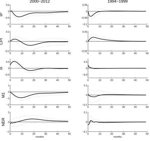
1.5 Effects of Monetary Policy during 1994-99 and 2000-12
This section compares the effect of monetary policy during the periods 1994-1998 and 2000-2012.
The idea of this section is to identify if the response of the system changed after the
implemen-tation of the inflation targeting and the flexible exchange rate. The goal is to characterize the
changes in the response. Using the benchmark specification detailed above the paper computes the
impulse response of output, prices, interest rate, M1 and nominal exchange rate to a 25 basis point
The estimation is constrained by the limited number of observations in the period
1994.09-1999.12. During 1994-1998 the Brazilian Real was pegged to a basket of currencies. The peg
system was replaced by a flexible exchange rate at the beginning of 1999. We extend the sample
period until the end of 1999 to allow the agents to incorporate the new policy. Figure 1.8 shows that
the effect of monetary policy are larger during the sample 2000.01-2012.12 than during
1994.09-1999.12. The main conclusions are: i) Response of the different variables during 1994-1999 was
around one tenth of the response observed during 2000-2012 and ii) The response of monetary
policy rate was less persistent. The weakness of the response of different variables during
1994-1999 is largely explained by the lack of credibility of the monetary regime and the high interest
rates driven by sovereign risk premiums.
Figure 1.8: Recursive Specification - 1994-1999 and 2000-2012
Impulse response function in percent points and the 90% confidence interval
0 10 20 30 40 50 −1 −0.5 0 0.5 2000−2012 IP
0 10 20 30 40 50 −0.2
0 0.2
CPI
0 10 20 30 40 50 −0.5
0 0.5
R
0 10 20 30 40 50 −2
−1 0 1
M1
0 10 20 30 40 50 −2
0 2
NER
months
0 10 20 30 40 50 −0.1
−0.05 0 0.05
1994−1999
0 10 20 30 40 50 −0.02
0 0.02
0 10 20 30 40 50 −0.5
0 0.5
0 10 20 30 40 50 −0.1
0 0.1
0 10 20 30 40 50 −0.1
0 0.1
1.6 Conclusions
Considering the Brazilian economy for the period 2000-2012, impulse response functions from
VARs point out that monetary policy has real effects on output and weak effects on prices in the
short and medium term. This implies that the estimation of a model that includes nominal rigidities
will better represent the Brazilian economy.
The second relevant conclusion is that the negative response of output is heterogeneous across
industries. We document that capital goods and durable goods present larger contractions after
a monetary policy tightening, while intermediate inputs and non-durable goods show small or no
responses to the same shock.
Finally this chapter documents that after the implementation of the inflation targeting and
flexible exchange rate framework, the main economic variables have become more sensitive to
Chapter 2
Monetary Policy and Market Interest Rates in Brazil
2.1 Introduction
The interest rate channel is one of the main transmission mechanisms of monetary policy. This
channel has been frequently studied for advanced economies. This chapter inquires about the
effectiveness of this mechanism for Brazil, where interest rate volatility is twice of that observed
in the United States1 and financial development is low.2 Specifically this chapter asks: i) How do
changes in the monetary policy rate affect longer3 term interest rates? and ii) Does the response of
market interest rates to changes in the monetary policy rate depend on the state of the economy?
Studying the Brazilian experience is relevant as it is one of the main emerging economies. Brazil
implemented structural reforms earlier than other emerging countries, therefore Brazil can set a
precedent for those countries. Among these reforms was the adoption of an inflation targeting
framework and a flexible exchange rate. These reforms stabilized the economy and set the interest
rate as the core monetary policy instrument.
1E.g. For the period 2000-2010, the standard deviation of the 1-year interest rate (Swap) in Brazil was 5.25%
while in the United States it was only 1.90%.
2E.g. For the period 2000-2010, domestic credit to the private sector was 39.5% of GDP in Brazil while in the
United States it was 190.8% of GDP. For the same period, the stocks traded were 24.9% of GDP while in the United States they were 242.8% of GDP.
3
By changing the relevant interest rates, the central banks can affect the short run output levels4.
The literature provides two main arguments for this. The first argument assumes a nominal
rigid-ity. Under this assumption changes in the monetary policy rate affect the real allocations of the
households and firms, at least in the short run. The second argument assumes that firms finance
their working capital with short term borrowing. By changing the interest rate the central bank can
modify the borrowing cost of firms and thus can modify the operational marginal cost. Therefore
output changes. A change in the 1-day interest rate alone (such as the monetary policy rate), with
no change in the longer term interest rates, will generate small or no intertemporal consumption
substitution and therefore no real effects. Similarly for the firms, the 1-day interest rate changes do
not significantly affect the firms’ behavior because the interest rates that matter for firms are the
rates used to finance inputs 6 to 12 month ahead. Then the relevant question is how the monetary
policy affects the relevant interest rate for households and firms. Understanding how the monetary
policy rate affects the relevant rates is crucial for the central banks.
This chapter will analyze the effects of monetary policy rate changes on the longer term interest
rates using high frequency (daily) data. Daily events data allow researchers to assume that variables,
such as prices and income, are given from one day to the next. The choice of daily data avoids
identification issues observed in monthly and quarterly data.5
This chapter explores how a change in the monetary policy rate (a 1-day interest rate) affects
the 3, 6, 9 and 12 month market interest rates. Specifically it will decompose the changes in the
monetary rate into anticipated and unanticipated components by using futures markets information.
It extends the previous literature in order to check if these results differ during economic expansions
and recessions. This is done using a Markov Switching estimation that allows the parameters to
be state dependent.
4
Christiano, Eichenbaum and Evans (1999), Bernanke and Blinder (1992), and Cushman and Zha (1997).
5
The main result is that in Brazil unanticipated shocks explain most of the changes in the longer
term interest rates, consistent with the literature on the United States (Kuttner (2001)). A
sec-ond relevant result is that the impact of unanticipated shocks is state dependent. In particular
unanticipated shocks have a larger impact during expansions. This asymmetry is attributed to the
longer expected duration of expansions and a stronger response of risk premia during recessions in
emerging economies.
2.2 Previous Studies
Previous papers have studied why long term rates respond to changes in short term rates and by
how much they respond in the United States, but the topic has been scarcely studied for emerging
economies.
2.2.1 Theoretical Perspective
The effects of short term interest rate changes on the long term interest rates are explained by the
expectation hypothesis. That hypothesis states that the longer term interest rates are a weighted
average of the current short term interest rate and the expected future short term interest rates,
plus a risk premium that is assumed constant.
rt(k) =
rt(1) (k+ 1) +
Pk
l=1Etrt+l(1) (k+ 1) +ρk
rt(k): interest rate in period t, with maturity k periods ahead.
ρk: risk premium.
Under the expectation hypothesis an increase in the monetary policy rate increases the short term
rate (rt(1)) and therefore increases the longer term interest rate (rt(k)). The expectation hypothesis
has been criticized because it assumes that the risk premium and the long term inflation are
constants. Assuming uncertainty about the future short term interest rates implies the risk premium
is changing and therefore it is a serious challenge to the expectation hypothesis. Although the
expectation hypothesis has been challenged, it can still explain a significant part of the movements
2.2.2 Empirical Perspective
Cook and Hahn (1988) looked at the effects of the changes in the monetary policy rates on the
term structure using daily events. By regressing the changes of the longer term interest rates on
the changes of the Fed Funds Target Rate, they found that a change in the target rate generates
large movements in the short term interest rate and smaller movements in long term interest rates.
Roley and Sellon (1995) argued that the relationship between long term and short term interest
rates depends on the stage of the business cycle. They argued that the effects of a change in the
Fed Funds Target Rate on long term rates would depend on how market participants interpret that
change. If the agents believe that the change in the target rate would be persistent, then long term
rates would respond more.
Cook and Hahn (1988) did not distinguish between the effects of anticipated and unanticipated
monetary policy actions. A second generation of studies, such as Kuttner (2001) and Cochrane
and Piazzesi (2002) considered the role of unanticipated monetary policy.6 These studies found
similar conclusions: 1) unanticipated changes in the monetary policy rate are the main drivers of
the movements in the longer term interest rates and 2) these effect are stronger for the shorter
maturities.
Gurkaynak, Sack and Swanson (2005) adopt a different approach. They stated that changes in
the target rate affect long term interest rates because they affect the expected long term inflation.
In particular since agents imperfectly predict long term inflation, thus unanticipated monetary
surprises imply adjustments in the expected long term inflation.7 They argue that the short term
interest rate will move in the same direction as the change in the monetary policy rate, due to the
expectation hypothesis. On the other hand the long term rates can move in the opposite direction
of the change in the monetary policy rate. This happens when agents perceive that the central
6
The main difference between Kuttner’s and Cochrane and Piazzesi’s studies is that Kuttner used futures markets data to measure unanticipated shocks, while Cochrane and Piazzesi used the change in the 1 month euro-dollar interest rate to measure monetary surprises.
7The idea is that long term inflation expectation is not strongly anchored. This goes against the standard argument
bank will change its long term inflation target with lags proportional to the current inflation. This
implies that as expected inflation goes down, the central bank may keep responding to current
inflation by raising the monetary policy rate and this results in a smaller long term inflation.
Beechey (2006) found that monetary policy surprises affect interest rates by changing the risk
premiums and not the expected future short term interest rate as argued by the expectation
hy-pothesis. Using an affine term structure model, Beechey found that a positive monetary surprise
increases the expected future short term interest rate but reduces the risk premium by an amount
sufficient to offset that increment. In a recent study Beechey and Wright (2009) decomposed the
effect of monetary surprises on nominal yields into the effect on the real interest rate and inflation
compensation. They conclude that after a positive monetary policy surprise inflation compensation
drops and the real interest rate rises.
The literature on monetary policy using daily events data is limited for emerging economies.
Larrain (2007) studied the effect of monetary surprises in Chile for the period 2001-2005. He
found that monetary policy surprises have significant but small effects on longer term interest
rates. For Brazil, Miranda Tabak (2003) documented the effects of monetary policy shocks on
the term structure of interest rates. He showed that changes in the target monetary policy rate
affect the 3, 6 and 12 months reference rates by using the change in the monetary policy target
rate as exogenous shocks for the period 1996-2001. In addition, Wu (2009) using Gurkaynak, Sack
and Swanson (2005) methodology found that the monetary surprises have significant effects for the
period 2004-2008 for Brazil.
2.3 Estimation
This section extends previous empirical evidence in terms of: 1) extending the sample and
2) performing an estimation that allows the parameter to depend on the state of the economy
2.3.1 Data
In Brazil the monetary policy rate is the SELIC rate.8 The SELIC rate is the nominal interest
rate at which banks trade reserves one day ahead using government securities as collateral. The
SELIC rate operates as the Fed Funds Rate does in the United States.
The limited development of the Brazilian financial market constrains the analysis of the term
structure to rates up to a year. The market interest rates for the Brazilian economy are the Swap
DIxPRE for 3, 6, 9 and 12 months. The sample period is January 2, 2003 until May 31, 20139 and
it includes 96 monetary policy committee meetings. In 67 of these meetings, the monetary policy
target rate was changed, while in the other 29 meetings monetary policy rate registered no change.
2.3.2 Estimating the Effect of Anticipated and Unanticipated Monetary Shocks
Changes in the monetary policy target rate are decomposed into anticipated and unanticipated
shocks using futures market data.10 Unanticipated monetary shocks are defined as the difference
between the target monetary policy rate (Rt) after the monetary policy committee meetings and
the expectation of the monetary policy rate (Et−1[Rt]) before these meetings. The expectation
of the monetary policy rate in period t is computed as the future contract on a close proxy rate
(future on CDI rate).11 Then the expectation of the SELIC isEt−1(Rt) = Future CDIt−1.12 Finally,
anticipated monetary policy shocks are defined as the difference between the change in the monetary
8
Portuguese acronym forSistema Especial de Liquida¸c˜ao e Custodia(SELIC) (Special Clearance and Settlement System).
9
The period 1999-2002 was excluded due to the extreme volatility in the financial markets generated by the Argentinian Crisis (2001-2002), the Brazilian election (2002) and in order to consider that before 2003 the central bank allowed the chair of the policy committee to change the target monetary policy rate outside of the monetary policy committee meetings.
10
Similar to Kuttner (2001).
11
The Certificate of Interbank Deposit (CDI is the Portuguese acronym) rate is the rate at which the banks exchange short term liquidity. CDIs are highly liquid assets and the CDI rate and the SELIC rate only differ because the SELIC rate requires Brazilian federal government bonds as collateral while the CDI rate does not requires Brazilian Fedeal government bonds as collateral. The correlation between both rates is 0.999. The future contracts on CDI is also a highly liquid asset. It is traded to insure financial agents against fluctuations in the domestic interest rates.
12
policy target rate and the unanticipated shock. Considering the definitions:
rjmt : j month market interest rate (Swap DIxPRE)
Rt: monetary policy target rate (SELIC target)
∆Rt: monetary policy shock (change in the monetary policy target rate)
Et−1(Rt): expectation on SELIC on the day of the committee meeting
∆Rtu: unanticipated monetary policy shock (∆Rut =Rt−Et−1(Rt)) ∆Rta: anticipated monetary policy shock (∆Rat = ∆Rt−∆Rut)
ξt iid∼N(0, σ)
It is possible to write the change of the j months maturity rate as:
∆rtjm=a+ba∆Rta+bu∆Rut +ξt
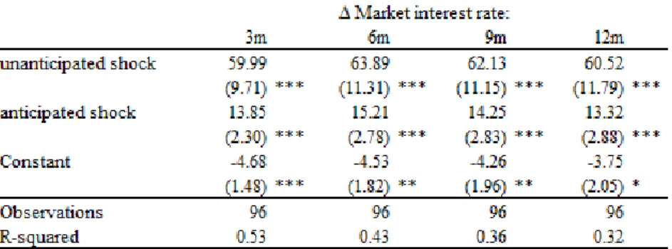
Table 2.1: Estimation - 2003-2013
The estimation shows that both shocks are statistically significant, but that unanticipated
mon-etary shocks explain a larger part of the changes in the 3, 6, 9 and 12 month interest rates. For
example, an unanticipated increase in the target rate of 100 basis points results in an increase of
60 basis points in the 12 months market interest rates. This result is consistent with Kuttner’s
estimations for the economy of the United States. The explanation for this response is the
expec-tation hypothesis. After an unanticipated shock, agents review their expecexpec-tations about the future
monetary policy rate and then long term rates respond. Results are also robust for different sample
2.3.3 Effects of Monetary Shocks During Recessions and Expansions
Background
This subsection explores whether the impact of anticipated and unanticipated monetary shocks
have similar magnitude during economic recessions and expansions. The intuition behind the
hypothesis is that the market interest rates respond differently during expansions and recessions
to unanticipated monetary shocks. The argument is based on: i) The expectation hypothesis
of interest rates and ii) The expected duration of expansion and recessions. Assuming there is
technological growth, expansions are longer than recessions. During expansions, agents expect that
after an increase in the monetary policy rate, the short term interest rates are expected to be high
(keep at the new level or go up) for a long period. Therefore long term rates will be affected more
because short term interest rates are expected to be higher for a long period. On the other hand,
during a recession agents expect that after a decrease in the monetary policy rate, the short term
interest rates are expected to return to their mean level within a few quarters, because historically
recessions are shorter than expansions. Hence the long term rates will be affected less because the
short term rates are expected to be lower for a shorter period.
A simple way to test this hypothesis is to split the sample in two subsamples and estimate the
coefficients. The sample was separated into a low state when the economy is in recession and
high state when the economy is in expansion. The period of expansion was measured using the
real GDP per capita in U.S. dollars. A recession is determined by two consecutive quarters of
contraction on the real GDP per capita in U.S. dollars. This criteria differs from the standard
NBER definition of two consequtive quarters of real GDP contractions. This allows us to consider
the effect of depreciation in the exchange rate. Sudden depreciation of the exchange rate in Brazil
signals periods of financial uncertainty at the early stages of recessions.
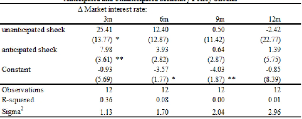
The regression results show that the response of the 3, 6, 9 and 12 months interest rates to
unanticipated shocks is larger during expansions (HIGH) than during recessions (LOW). Although
Table 2.2: Subsample Estimation - 2003-2013
coefficients in the two states (Ho: βLow−βHigh= 0).
The approach of spliting the sample is subject to the issue that the state of the economy is
subject to uncertanty. During certain periods of time it is not easy to determine if the economy is
in an expansion or a recession. This is known expost, after data is released. In the best case the
agents asign probabilities of being in each state at each time. In order to consider this issue in the
following subsection the paper follows an approach that allows us to estimate the probability of
being in each state and the parameters of the responses.
Estimation
In order to measure these effects, this paper estimates a two state regime model similar to
Hamilton (1988). The two states are “Low” and “High”. In the “Low” state, the economy is in a
recession, while in the “High” state, it is in an expansion. The methodology jointly estimates the
parameters in each state and the probability of being in each state.
The state of the economy (St) can be either an “High” (H) or a “Low” (L). In state H the
parameters will be different from the parameters in state L:
∆rjt =aL+ba,L∆Rta+bu,L∆Rtu+ξt,L ξt,L
iid
∼N(0, σL2)
∆rtj =aH +ba,H∆Rta+bu,H∆Rut +ξt,H ξt,H
iid
The state of the economy St is not directly observable, but it is possible to parameterizeSt by
St∗ which is measured with error. Assume:
St=
L if S∗≤0 H if S∗>0
The state St is parametrized as St∗=az+bzZt+etwhere:
Zt=IPt−T rendt
IPt: Industrial Production index SA13
T rendt: Industrial Production Hodrick-Prescott filter
et
iid
∼N(0,1): measurement error
Then the probability in state “Low” and “High” are defined as:
P(St=L) = P(S∗≤0)
= P(az+bzZt+et≤0) = P(et≤ −az−bzZt) and
P(St=H) = 1−P(S∗≤0)
Given this information the likelihood function is defined as:
LL =
T
X
t=1
[f(Yt|Xt, St=L;θL)P(S =L|Zt;θZ) +f(Yt|Xt, St=H;θH)P(S =H|Zt;θZ)]
Where:
Yt∈
∆rt3m∆rt6m∆r9tm∆r12t m
Xt={∆Rat,∆Rut}
θH ={aH, ba,H, bu,H, σH}
13
θL={aL, ba,L, bu,L, σL}
θZ={az, bz}
f(Yt|Xt, St=L;θL) =φ
∆rjt−aL−ba,L∆Rat−bu,L∆Rut
σL
f(Yt|Xt, St=H;θH) =φ
∆rjt−aH−ba,H∆Rat−bu,H∆Rut
σH
P(S =L|Zt;θZ) = Φ(−az−bzZt)
φ(.)≡ pdf of a normal standard Φ(.)≡cdf of a normal standard
The estimation is performed through a Expectation - Maximization (EM) algorithm. The idea
of this method is described in the following steps:
1. Given an initial guess ofθ0
Z,P(S =L|Zt;θ0Z) is computed (where 0 is the initial estimation counter).
2. The parametersθ0
L andθ0H are estimated by maximizing the LL given θ0Z.
3. Using θ0
L and θH0 the parameters θ1Z are estimated by maximizing the LL given θL0 and θH0 and
P(St=L|Zt;θZ) is re-computed.
4. The parametersθ1
L andθ1H are estimated givenθZ1.
The process continues by repeating steps 2-4 until the algorithm finds convergence between the
parameters (i.e. θkM −θkM−1 = 0, for M=H,L,Z).
The log-likelihood function shows several local maximums. For this reason a grid search for the
parameters was applied to find the global maximum. Appendix B.2 shows a representation of the
Log-likelihood using the two sensitive parameters (aZ,bZ) as support.
Table 2.3 presents the results. The estimation signals that the effects of unanticipated shocks on
interest rates are larger during expansions. That is, an unanticipated shock of a 100 basis points
during an expansion has an effect of 84 basis points in the 12 month interest rate, while it has no
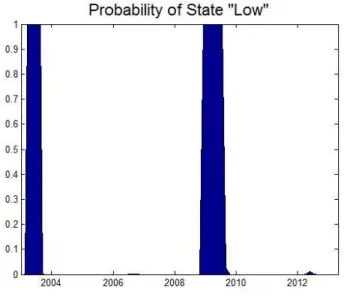
significant impact during a recession. Finally Figure 2.1 shows the probability of being in state
“Low” estimated with the 3 month interest rates. The probabilities for the other interest rate terms
are similar as the parameters of the cumulative distribution function are similar (as shown in Table
Table 2.3: State Dependent Estimation - 2003-2013
Robustness test show similar results (See Appendix B.3), but the limited sample size makes the
Figure 2.1: Sample 2003-2013 - 3-Month Interest Rate
2.4 Conclusions
This chapter examines the interest rate channel and concludes that it is an active transmission
mechanism of monetary policy in Brazil. This conclusion was reached based on high frequency
data, which shows that unanticipated changes in the monetary policy rate result in changes in
the market interest rates. Estimations show that the 12 month rate responds by 60 basis points
to an unanticipated monetary shock of a 100 basis points. Using a state dependent estimation
for recessions and expansions, evidence shows that these responses are not homogeneous during
expansions and recessions. Expansions are associated with higher responses of interest rates to
unanticipated monetary policy shocks. In particular the estimation shows that an unanticipated
monetary shock of a 100 basis points increases the 12 month interest rate by 79 basis points, while
the same shock in a recession has no significant impact.
During recessions the effectiveness of interest rate channel seems to be weaker. The response of
interest rate to unanticipated changes in the monetary policy rate is weak because the recession
is expected to last a few quarters. In constrast during expansions, unanticipated changes in the
monetary policy rate are expected to have longer effects as expansion have historically been longer
Chapter 3
Working Capital, Financial Frictions and Monetary Policy
3.1 Introduction
The working capital constraint states that firms are required to borrow to finance wages and
inputs before output is sold. In this way the interest rate directly affects the cost of the firms and
generates what is known as the working capital channel or cost channel of monetary policy. This
implies that interest rate movements affect the aggregate supply.
The working capital channel and the traditional interest rate channel affect inflation in opposite
directions, leaving open the question about the final effect of a monetary shock on inflation. Via
the interest rate channel, an increase in the interest rate will reduce output and afterwards it will
reduce inflation (mainly affecting aggregate demand). Through the cost channel of monetary policy,
an increase in the interest rate will increase the cost of the firms and therefore will raise inflation.
In a closed economy the effect on inflation is ambiguous; it depends on the size of both the interest
rate channel and the working capital channel of monetary policy. The larger the proportion of
working capital that is financed with credit, the stronger the cost channel will be.
This chapter inquires about the size of these channels in an open economy. In such environment
a monetary tightening implies contractions on output and prices that are larger than in a closed
economy. This is attributed to the exchange rate channel, which generates a short term appreciation
of the domestic currency and therefore a substitution between domestic and foreign goods. Thus
the interest rate channel and the exchange rate channel might dominate any effect of the working
This chapter asks: If there is an increase in the proportion of the working capital financed with
credit, what are the implications for monetary policy in an open economy? From the central bank’s
perspective, what is the difference between an expansion of working capital lending in a closed
economy and the same expansion in an open economy? How does the sensitivity of economic
variables (such as output and inflation) to monetary policy change in the presence of a working
capital channel?
This chapter is motivated by the recent changes in the financial behavior of the firms in Latin
America and in particular in Brazil. Data indicate that in several Latin American countries, the
share of working capital financed with credit has increased1 (Table 3.1). In Brazil firms financed
43.7% of working capital with credit in 2006, compared with 54.4% in 2010. Credit lines that
finance working capital2 increased from 1.3% of GDP in 2000 to 8.5% of GDP in 2012 (Figure 3.1)3
and they explain more than half of the commercial bank lending to firms.
Table 3.1: Percent of Working Capital Financed with Credit
Country 2006 2010 Diff.
Brazil 43.7 54.4 10.7
Colombia 46.8 57.3 10.5
Peru 46.2 55.5 9.4
Argentina 30.6 40.0 9.3
Uruguay 24.0 32.6 8.6
Bolivia 31.0 37.3 6.2
Paraguay 34.7 36.7 2.1
Ecuador 45.5 46.6 1.1
Chile 41.5 42.5 1.0
Venezuela 14.3 13.4 -0.9
Source: based on World Bank, Enterprise Surveys.
An important feature of working capital credit is that it is a short term lending consistent
with the lack of domestic long term funding in emerging economies documented by the original
1Based on the World Bank Enterprise Surveys, which record financial sources of working capital. The financial
sources are based on information collected during interviews with the management of firms.
2A wider definition of working capital credit can also include domestic trade credit, but This chapter follows the
central bank’s definition to simplify. Some caution is needed if foreign trade credit lines are included in the working capital credit definition. Foreign trade credit is funded by foreign banks and suppliers whose lending is less sensitive to domestic monetary policy.
3This rise is mainly explained by the inflation stabilization and the financial development observed since 1999.
Figure 3.1: Lending to Firms in Brazil
sin literature (Eichengreen, Hausmann and Panizza (2003)). According to that research, firms in
emerging economies can only access long term financing in foreign currency. While short term
financing was mostly in foreign currency in the early 1990s in many emerging economies, this has
changed since the early 2000s in some Latin American countries. In Brazil, nowadays a large part
of the short term borrowing by the firms is done through the domestic banking sector4. Thus
focusing on short term lending in domestic currency for Brazil is a sensible assumption that allows
for the original sin argument, but restricts the original sin to long term financing5.
Financial frictions have a critical role amplifying the working capital channel. In developing and
emerging economies, spreads between lending and borrowing interest rates are important and reflect
financial frictions. In Brazil the spreads move in the same direction as the monetary policy rate.
The spreads amplify the effect of the interest rate in the cost of the firms. Financial frictions make
domestic inflation less sensitive to a monetary shock because they strengthen the cost channel.
The main contribution of this chapter is to analyze the effects of introducing working capital in a
small open economy with financial frictions. This chapter applies a general equilibrium framework
in order to explain the potential consequences of specific and concrete structural changes that are
taking place in Brazil. The main results are that: i) When the economy is more open, the working
4
In Brazil foreign currency bank lending is banned by law.