Essays on Teacher Mobility
Jeremy A. Cook
A dissertation submitted to the faculty of the University of North Carolina at Chapel Hill in partial fulfillment of the requirements for the degree of Doctor of Philosophy in the Department of Economics.
Chapel Hill 2012
Approved by:
Donna Gilleskie
David Guilkey
Clement Joubert
Brian McManus
Abstract
JEREMY A. COOK: Essays on Teacher Mobility. (Under the direction of Donna Gilleskie.)
The allocation of quality teachers across schools is of interest because of both the
impor-tance and costliness of teachers as inputs in the education production process. Furthermore,
because teachers have preferences over their workplace characteristics, this allocation across
schools is nonrandom. This research examines teacher mobility within the school system by
fo-cusing on the school characteristics that a↵ect the probability of teachers leaving their current
schools. Using longitudinal data on public schools in North Carolina, I estimate teacher
mobil-ity probabilities using empirical specifications that incorporate current school characteristics,
as well as characteristics of other potential schools.
I jointly estimate these teacher mobility probabilities with two endogenous teacher
creden-tial outcomes. The joint estimation uses a discrete factor random e↵ects method to control
for both individual permanent and time-varying unobserved heterogeneity. Results show that
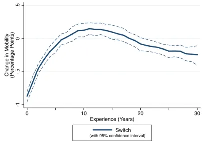
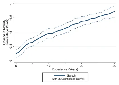
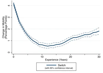
changes in student demographics have significant e↵ects on one-year mobility probabilities.
These changes in demographics have di↵erent e↵ects across teachers of di↵erent experience
levels, with teachers early in their careers being more sensitive to changes in student
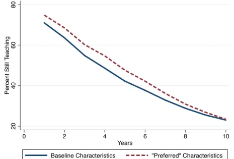
charac-teristics and salary than more experienced teachers. Long run results suggest that providing
beginning teachers with preferred school characteristics may result in a substantial increase in
Acknowledgments
I am very grateful for the opportunity to pursue a graduate degree at the University
of North Carolina at Chapel Hill. I would like to thank the members of my dissertation
committee for their influence and helpful comments at many stages of this research. Most
notably, I am indebted to my dissertation advisor, Donna Gilleskie, for taking me on as an
advisee. Her feedback and encouragement made a significant contribution to my experience,
especially during this past year.
My cohort of economics graduate students at UNC-CH made this experience more enjoyable
and memorable. I am appreciative of the camaraderie we shared that eased the burden of the
various challenges of a doctoral program.
I am most thankful for my faithful friends and family. Their prayers and encouragement
provided me with a renewed perspective during the tougher times. This dissertation is
dedi-cated to my family. I am deeply grateful for their unwavering love and support, especially that
of my parents who have sacrificed so much for their children, and my brother, for always lifting
my spirits. Finally, I am exceptionally thankful for Abigail and her encouragement, patience,
Table of Contents
List of Tables . . . viii
List of Figures . . . x
1 Introduction . . . 1
2 Relevant Literature . . . 5
2.1 Teacher Mobility . . . 5
2.1.1 Teacher Attrition . . . 5
2.1.2 Mobility within the Profession . . . 6
2.2 Teacher Quality . . . 8
3 Theoretical Motivation . . . 11
3.1 Teacher Decisions . . . 11
4 Empirical Model . . . 16
4.1 Teacher Outcomes . . . 16
4.2 District Level Mobility . . . 16
4.3 Estimation Technique . . . 19
4.5 The Likelihood Function . . . 22
4.6 School Level Mobility . . . 24
4.6.1 Random Sampling of Alternatives . . . 25
4.6.2 Subsample of Teachers . . . 27
5 Data . . . 29
5.1 Description . . . 29
5.2 Sample Selection . . . 31
5.3 Subsample of Teachers . . . 36
6 Results . . . 37
6.1 District Level Model Results . . . 37
6.1.1 Marginal E↵ects . . . 37
6.1.2 Long Run E↵ects . . . 46
6.2 School Level Model Results . . . 48
6.2.1 Random Sampling of Alternatives . . . 48
6.2.2 Subsample of Teachers . . . 53
6.3 Comparison of Models with and without Non-pecuniary Characteristics . . . . 59
7 Discussion . . . 66
7.1 Limitations and Future Research . . . 67
A Variable Descriptions . . . 72
C Model Results . . . 79
C.1 District Level Model Results . . . 79
C.1.1 Supplemental Figures . . . 88
C.2 School Level Model Results . . . 97
C.3 School Level Model Results using Subsample of Teachers . . . 98
C.4 School Level Model Results using Subsample of Teachers (without controlling for unobserved heterogeneity) . . . 109
List of Tables
5.1 Selected School Characteristics of Switching Teachers . . . 35
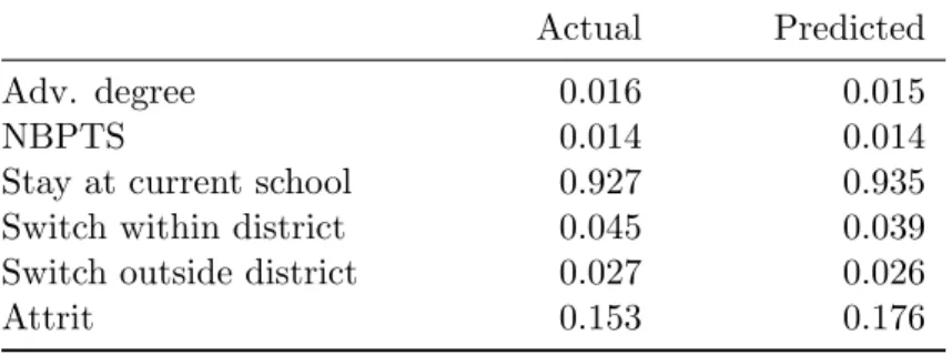
6.1 District Level Model Fit: Predicted Outcomes versus Observed Outcomes . . . 38
6.2 Baseline Probabilities . . . 39
6.3 Marginal E↵ects of Increased Students on Free/Reduced Lunch . . . 40
6.4 Marginal E↵ects of Increased Black Students . . . 41
6.5 Marginal E↵ects of Increased Salary . . . 42
A.1 Description of Variables . . . 72
B.1 Summary Statistics: Teacher Characteristics . . . 75
B.2 Summary Statistics: School and Community Characteristics . . . 76
B.3 Sample Entry and Attrition . . . 77
B.4 Length in Sample . . . 78
C.1 District Level Estimation Results: Teacher Credential Outcomes (jointly esti-mated with attrition and mobility equations) . . . 79
C.2 District Level Estimation Results: Teacher Mobility Outcomes (jointly esti-mated with credential equations) . . . 82
C.3 District Level Estimation Results: Unobserved Heterogeneity . . . 86
C.4 District Level Estimation Results: Initially Observed Values . . . 87
C.6 District Level Estimation Results: Teacher Mobility Outcomes (without unob-served heterogeneity) . . . 93
C.7 School Level Estimation Results: Teacher Mobility Outcomes . . . 97
C.8 Model Fit: Predicted Outcomes versus Observed Outcomes . . . 98
C.9 School Level Subsample Estimation Results: Teacher Credential Outcomes (jointly estimated with mobility and attrition equations) . . . 99
C.10 School Level Subsample Estimation Results: Teacher Attrition Outcome (jointly estimated with credential and mobility equations) . . . 101
C.11 School Level Subsample Estimation Results: Teacher Mobility Outcomes (jointly estimated with credential and attrition equations) . . . 103
C.12 School Level Subsample Estimation Results: Unobserved Heterogeneity . . . . 104
C.13 School Level Subsample Estimation Results: Teacher Attrition Outcome (with-out unobserved heterogeneity) . . . 109
List of Figures
3.1 Timing of Behavior . . . 13
5.1 Teaching Experience . . . 32
5.2 Credential Outcomes . . . 33
5.3 Mobility Outcomes . . . 34
6.1 District Level: Marginal E↵ect of Pct. Lunch on Mobility . . . 43
6.2 District Level: Marginal E↵ect of Pct. Black on Mobility . . . 43
6.3 District Level: Marginal E↵ect of Salary on Mobility . . . 44
6.4 District Level: Marginal E↵ect of Pct. Lunch on Attrition . . . 44
6.5 District Level: Marginal E↵ect of Pct. Black on Attrition . . . 45
6.6 District Level: Marginal E↵ect of Salary on Attrition . . . 45
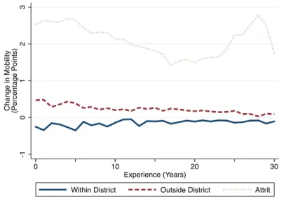
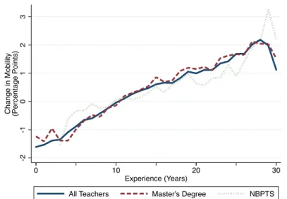
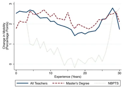
6.7 District Level: Long Run E↵ects . . . 47
6.8 School Level: Marginal E↵ect of Pct. Lunch at Current School . . . 50
6.9 School Level: Marginal E↵ect of Pct. Black at Current School . . . 50
6.10 School Level: Marginal E↵ect of Salary at Current School . . . 51
6.11 School Level: Marginal E↵ect of Pct. Lunch at Other Schools . . . 52
6.12 School Level: Marginal E↵ect of Pct. Black at Other Schools . . . 52
6.13 School Level: Marginal E↵ect of Salary at Other Schools . . . 53
6.15 School Level Subsample: Marginal E↵ect of Pct. Black at Current School . . . 56
6.16 School Level Subsample: Marginal E↵ect of Salary at Current School . . . 57
6.17 School Level Subsample: Marginal E↵ect of Pct. Lunch at Other Schools . . . 58
6.18 School Level Subsample: Marginal E↵ect of Pct. Black at Other Schools . . . . 58
6.19 School Level Subsample: Marginal E↵ect of Salary at Other Schools . . . 59
6.20 Model Comparison: Marginal E↵ects of Increasing Pct. Lunch Switching Within District . . . 61
6.21 Model Comparison: Marginal E↵ects of Increasing Pct. Lunch Switching Out-side District . . . 62
6.22 Model Comparison: Marginal E↵ects of Increasing Pct. Lunch Attrition . . . . 62
6.23 Model Comparison: Marginal E↵ects of Increasing Pct. Black Switching Within District . . . 64
6.24 Model Comparison: Marginal E↵ects of Increasing Pct. Black Switching Out-side District . . . 64
6.25 Model Comparison: Marginal E↵ects of Increasing Pct. Black Attrition . . . . 65
C.1 District Level: Marginal E↵ect of School Characteristics on Attrition . . . 88
C.2 District Level: Marginal E↵ect of School Characteristics on Within District Mobility . . . 88
C.3 District Level: Marginal E↵ect of School Characteristics on Out of District Mobility . . . 89
C.4 School Level Subsample: Marginal E↵ect of Pct. Lunch at Current School (without unobserved heterogeneity) . . . 112
C.6 School Level Subsample: Marginal E↵ect of Salary at Current School (without unobserved heterogeneity) . . . 113
C.7 School Level Subsample: Marginal E↵ect of Pct. Lunch at Other Schools (with-out unobserved heterogeneity) . . . 113
C.8 School Level Subsample: Marginal E↵ect of Pct. Black at Other Schools (with-out unobserved heterogeneity) . . . 114
1 Introduction
The e↵ect of school resources on human capital accumulation is a topic that has been intensely
studied over the past several decades across di↵erent disciplines. While research has shown
that formal schooling is only one component of a complex production process that involves own
ability, family, and peers, it is arguably the component most directly a↵ected by government
legislation and public funding. During the 2008 fiscal year, average state spending on primary
and secondary education comprised 23.6% of total state direct general expenditures.1 Over
the past 50 years, national real spending on public education has increased by an average of
7% annually.
Educational instruction is the most costly school resource by a large margin. In 2008 teacher
salaries and benefits exceeded 55% of all public school expenditures.2 Given the expense of
this resource, it is no surprise that teacher quality and its e↵ect on the academic outcomes
of students is of interest to school administrators, parents, taxpayers, and policy-makers.
Beginning with the 1966 “Coleman Report”, numerous studies have attempted to quantify
the e↵ect of school resources, with special attention to that of teacher quality. Although this
literature is divided over which observable characteristics embody teacher quality, there is a
consensus among recent studies that teacher quality is the most important resource used by
public schools (Hanushek, 1986; Ehrenberg and Brewer, 1994; Rocko↵, 2004).
Much of the current literature treats teacher quality as an exogenous, or randomly
deter-mined, characteristic within a school. However, unlike most other school resources, teachers
have preferences over characteristics of their place of employment, hence the composition of
teachers, and thus teacher quality, is not random across schools. Several studies show that
1National Center for Education Statistics: Digest of Education Statistics: 2010, Table 31
teachers self-select across schools, oftentimes with more highly qualified teachers working at
schools with better resources, lower poverty rates, and fewer minority students (Lankford,
Loeb, and Wycko↵, 2002; Clotfelter, Ladd, and Vigdor, 2005). Studies that ignore this
non-random sorting of teachers produce biased estimates of the e↵ect of teacher quality on student
achievement outcomes.
Based on evidence that teachers are important, expensive, and non-randomly placed
in-puts, their mobility between schools is worth studying. The primary goal of this research is
to examine the determinants of teacher mobility. Specifically this study focuses on the
stu-dent, school, and district characteristics that influence teacher movements between schools and
school districts. I use three empirical approaches to examine this mobility. My first approach
uses a multinomial logit model to estimate the mobility probability. This “district level”
anal-ysis restricts the mobility outcome to either stay in the current school, switch to another school
within the same district, switch to another school in a di↵erent district, or leave the school
system.
The second and third empirical approaches expand the mobility outcome to include specific
school selection. These “school level” analyses use a conditional logit framework with specific
schools in the set of mobility alternatives. With these models, regressors vary by alternative,
allowing the characteristics of potential schools to a↵ect the probability of leaving a teacher’s
current school. The second empirical approach uses the entire sample of teachers and does
not allow for unobserved heterogeneity. The third empirical approach controls for unobserved
heterogeneity and uses a subsample of high school teachers from the Piedmont region of North
Carolina. In this model, the set of alternatives includes all high schools in this region.
This research adds to the current literature in several ways. First, I use a dynamic
frame-work to jointly estimate the teacher mobility outcome along with endogenous teacher credential
outcomes over time. These credentials, often associated with teacher quality, include outcomes
for obtaining an advanced degree and becoming certified by the National Board for
Profes-sional Teaching Standards (NBPTS). Teaching experience is also modeled through mobility
and attrition outcomes. Several studies in the literature have focused on these credentials
may influence the decision to seek credentials, as well as a↵ect school selection, recovery of
unbiased e↵ects requires joint estimation of these outcomes. In order to reduce possible bias
due to unobserved characteristics in the joint estimation, I use a discrete factor random e↵ects
method that accounts for both individual (teacher) permanent and time-varying unobserved
heterogeneity.
Second, by using a conditional logit framework this research presents a more comprehensive
examination of the determinants of teacher mobility. If teachers are voluntarily leaving their
current school for another school, the arrival school characteristics may play an important
role in that outcome. Specifying the probability of leaving the current school as a function of
both current school characteristics as well as possible future school characteristics introduces
a measure of the “pull” aspect of the arrival school characteristics.
Third, the data I use are longitudinal administrative data on the North Carolina public
school system which include unique information on the non-pecuniary benefits of teaching at a
particular school. The existing literature in this area often uses student characteristics such as
race and poverty level to proxy for poor working conditions. The data I use are supplemented
with a working conditions survey administered to teachers. The survey contains teacher
re-sponses regarding topics such as school safety, administration relationships, and professional
development opportunities. The inclusion of these data help mitigate the potential bias due
to unobserved variables that are correlated with student race and poverty characteristics.
The results of this research show that changes in student demographics have significant
e↵ects on teacher mobility, and that these e↵ects vary across teachers with di↵erent levels of
teaching experience. For example, the results from one model show that an increase in the
proportion of black students of 25 percentage points decreases the probability of a teacher
staying at her current school by up to 2.8 percentage points for teachers with five or fewer
years of experience, compared to 1.4 percentage points for more experienced teachers. These
changes in teacher mobility are one-year transition rates. Over time, these changes in school
characteristics can have a much larger e↵ect on teacher mobility and attrition.
Potentially, biases still remain in the results of this research. These biases arise from the
that a teacher’s employment opportunities, reflected by the discrete alternatives of the mobility
equations, are exogenous. Realistically, the mobility of an individual is constrained by the set
of o↵ers an individual receives. Ignoring these restrictions may result in biased estimates of
mobility probabilities. The potential biases from this assumption are discussed further in
Chapter 7.
The remainder of this dissertation is organized in the following structure. Chapter 2
discusses the literature related to teacher mobility and teacher quality. Chapter 3 introduces
the general theoretical motivation for the empirical models. Chapter 4 discusses each of the
empirical specifications used in estimation. Chapter 5 describes the North Carolina data and
the sample of teachers used in the analyses. Chapter 6 presents the estimation results from
these di↵erent models. Finally, Chapter 7 provides a discussion of this research, including its
limitations and the potential biases that may be present. It also discusses the direction of
future research. Additional data summaries and all estimated coefficients are included in the
2 Relevant Literature
There are two areas of the education economics literature that relate to my research. The first
area covers teacher mobility. This literature examines the determinants of teacher movement
into the profession, between schools, and attrition from teaching. The second area is teacher
quality, which is concerned with identifying the characteristics that define or a↵ect teacher
quality, and the e↵ect of these characteristics on student achievement.
2.1 Teacher Mobility
2.1.1 Teacher Attrition
Several studies focus on the retention of teachers in the teaching profession. Ingersoll and Smith
(2003) argue that retaining quality teachers is a much more difficult task than recruiting new
teachers. Stinebrickner (2001) uses the NLS-72 to estimate a structural dynamic discrete choice
model of attrition from the teaching profession. He finds that changes in family characteristics
such as marital status and number of children are the most important predictors of attrition.
In addition, he finds that attrition is responsive to wage increases, and that teachers with
better academic traits obtain higher wages in alternative professions. Using the same data
and a competing risks duration specification, Stinebrickner (2002) again finds that attrition
is highly correlated with changes in family structure. He also notes that exit rates out of the
teaching profession are lower than those of non-teachers’ first job. Exit rates out of the labor
force entirely are similar for teachers and non-teachers. Using the NLS-72, van der Klaauw
(1999) also finds salaries and alternative wages influence teacher retention rates. Dolton and
van der Klaauw (1999) use a sample of UK university graduates to examine teacher career
decisions for the first six years of their career. Using a competing risks model they find that
the profession by 5 percentage points.
2.1.2 Mobility within the Profession
Greenberg and McCall (1974), in one of the earliest economic studies to examine teacher
mobility between schools, analyze the one-year (1971-1972) transition of teachers within the
San Diego school system. Using an OLS linear probability model, they estimate the probability
of a teacher leaving her current school. The probability of a teacher transferring from a school
with below-average socio-economic status (SES) was approximately twice the probability of
transferring from a school with average SES. They find that more experienced and more
educated teachers tend to leave schools with low SES characteristics. Teachers moving between
schools tend to move to schools with higher SES characteristics.
Lankford, Loeb, and Wycko↵ (2002), Boyd, Lankford, Loeb, and Wycko↵ (2005) and
Boyd, Lankford, Loeb, and Wycko↵(2003) examine teacher sorting using administrative data
from the state of New York. In their descriptive study, Lankford, Loeb, and Wycko↵ (2002)
summarize the variation in teacher characteristics across schools and regions from 1985-2000.
They show that di↵erences in teacher qualifications are most prominent at the school level
rather than at the regional level. Among teachers who transition between schools after 1992,
they find that the proportion of minority and poor students at the departing school is between
75 and 100 percent greater than that of the arrival school. They also find that, on average,
teachers who move to a new school have a higher quality skill set than those who stay. Boyd,
Lankford, Loeb, and Wycko↵(2005) use the same data to investigate teacher preferences over
region. They observe that between the years 1999 - 2002 61 percent of teachers accepted their
first teaching assignment within 15 miles of where they attended high school, and 85 percent
within 40 miles. In addition, they found that teachers were likely to accept jobs in towns with
characteristics similar to their hometown.
Boyd, Lankford, Loeb, and Wycko↵(2003) employ a two-sided matching model of teachers
and schools using the initial assignments of teachers in five New York metropolitan areas. They
find that teachers with higher qualifications are more likely to be matched with higher wages
1.3 standard deviations would be needed to o↵set the decrease in utility from a 0.46 standard
deviation increase in minority students.
Using Texas administrative data on elementary school teachers, Hanushek, Kain, and
Rivkin (2004) examine the probabilities of teachers moving within or outside of their
cur-rent school district. They find that in order to keep a non-minority teacher from leaving, a
10 percent increase in minority students would require a 10 percent increase in salary. On
average, a 10 percent increase in salary reduced the probability of leaving by approximately
3 percentage points for teachers with five or fewer years of experience. They also find that
salary has a larger influence on switching within Texas schools than it does on leaving Texas
schools.
In a similar study, Scafidi, Sjoquist, and Stinebrickner (2007) examine teachers in Georgia
public elementary schools. Focusing on new teachers, they estimate a competing risks model
with the options of switching schools/districts, taking an administrative job, taking a job
within Georgia outside the public schools system, or leaving the Georgia labor force. They
find that increasing the proportion of black students by one standard deviation increases the
probability of a teacher leaving by 6.5 percentage points. They also find that black teachers
are less likely to leave schools with a high proportion of minority students than white teachers.
Furthermore, they find only a weak correlation between salary and the probability of leaving
a school, contrasting the results of previous studies.
Jackson (2009) estimates the e↵ect of changes in student demographics on the composition
of teacher characteristics of a school using a natural experiment in one school district in
North Carolina. In 2002, Charlotte-Mecklenburg schools ended their integration-based busing
policy, leading to an immediate change in student demographics within each school. He uses
a di↵erence-in-di↵erences technique along with similar school districts to uncover the causal
e↵ect of these changes on teacher composition. He finds that a 10 percentage point increase in
black students results in a decrease in the average experience level of teachers of 0.8 years. He
also finds that schools with a higher proportion of black students did not have higher teacher
2.2 Teacher Quality
One of the most often cited results of James Coleman’s “Equality of Educational Opportunity”
is that peer and family characteristics are far more important than school resources. The
complexity of human capital accumulation combined with the lack of comprehensive data
make valid estimation of each component’s e↵ect difficult (Todd and Wolpin, 2003). In light
of this complexity, measuring the e↵ect of teacher quality has led to a variety of conclusions
in the literature. While the modern literature disagrees on which observable characteristics
signify teacher quality, they do overwhelming agree that teacher quality is the most important
school resource in predicting student outcomes. Hanushek (1986) articulates the inconclusive
results of this literature when he writes that it is “difficult if not impossible to specify a few
objective or subjective characteristics of teachers that capture the systematic di↵erences of
both backgrounds of teachers and their idiosyncratic choices of teaching styles and methods.”
There are severable observable teacher characteristics that have been associated with
teacher quality in the literature. These characteristics usually fall under the categories of
pre-teaching human capital (quality of undergraduate institution, major, GPA, test scores)
and human capital measures obtainable while teaching (experience, master’s degree, nation
board certification, licensure).
Summers and Wolfe (1977) examine a 1970-1971 randomly selected sample of schools and
students from the Philadelphia Public School District. They find a positive correlation between
the selectivity of a teacher’s undergraduate institution and student achievement. Ehrenberg
and Brewer (1994) also come to this conclusion using data from the 1980 High School and Beyond survey. Ferguson and Ladd (1996) examine the e↵ect of teacher quality at both the student and aggregate school level. They use Alabama fourth grade students in the 1991
academic year. They find that a one standard deviation in teacher test scores increases student
test scores by 0.1 standard deviations. Their results also show a one standard deviation
increase in the percent of teachers with a masters degree increases student test scores by
0.026 standard deviations. They did not find a significant e↵ect of experience on student
with a masters’ degree in math and student math achievement. Kukla-Acevedo (2009) uses
Kentucky data to analyze the e↵ects of teacher preparation on student outcomes. She finds
the teachers’ undergraduate GPA is a significant predictor of student math scores, with a one
standard deviation increase in math GPA resulting in a 0.385 standard deviation increase in
math scores for minority students.
Several studies provide evidence of a positive correlation between teachers accredited with
the National Board for Professional Teaching Standards (NBPTS) and student achievement.
Goldhaber and Anthony (2007) examine data on NBPTS applicants in North Carolina from
1997 to 2000. They find that while the NBPTS accreditation process does not necessarily result
in improved teacher quality, the process does successfully identify applicants who are higher
quality teachers. Successful applicants to the process are shown to have a larger influence
on student achievement than unsuccessful applicants. Using administrative data on a Florida
school district, Cavalluzzo (2004) also found support for NBPTS certification as a signal of
teaching quality. Vandevoort, Amrein-Beardsley, and Berliner (2004) find similar results,
although their sample consists of Arizona teachers, of which only 35 were NBPTS certified.
The most common teacher characteristic found to be significant in the literature is teaching
experience (Kane, Rocko↵, and Staiger, 2008; Aaronson, Barrow, and Sander, 2007; Rivkin,
Hanushek, and Kain, 2005; Ballou and Podgursky, 1997; Loeb and Page, 2000; Rocko↵, 2004).
Both Rivkin, Hanushek, and Kain (2005) and Rocko↵(2004) find that the first few years of
teaching experience have a significant e↵ect on student achievement, with the positive e↵ect
diminishing as experience increases.
Several studies conclude that observable teacher characteristics other than experience are
not correlated with student achievement. Aaronson, Barrow, and Sander (2007) estimate
sev-eral value-added models using cross-sectional data from the Chicago Public School system.
They find only a weak correlation between teacher observable characteristics such as an
ad-vanced degree and teaching certification with student achievement. Rivkin, Hanushek, and
Kain (2005) find similar results using Texas administrative data. They find no significant
cor-relation between a teacher’s education credentials. They find a positive corcor-relation between
teaching.
The e↵ect of school resources on student achievement varies substantially across di↵erent
data and methods. One noticeable di↵erence is between studies using student-level data and
studies aggregating at the school, district, or even state level. Studies that have used aggregate
data tend to find more positive significant correlations between school resources and student
achievement (Card and Krueger, 1992). These correlations tend to be larger than those found
in studies using student level data. Loeb and Bound (1996) and Card and Krueger (1992)
argue that aggregation can reduce measurement error commonly associated with test score
data. Loeb and Bound (1996) also note that aggregation at the school level better accounts
for the entirety of school resources over a students education. Aggregation may also help to
mitigate endogenous sorting of resources between classrooms. If there are omitted variables at
the level of aggregation, such as di↵erences in state policies, aggregation can increase
omitted-variable bias (Hanushek, Rivkin, and Taylor, 1996). Aggregation is likely to lead to greater
bias in estimated marginal e↵ects of inputs if those inputs are endogenous. For example,
average teacher quality at a school is likely correlated with unobserved teacher preferences.
None of these papers attempting to measure the e↵ects take into account the endogeneity of
3 Theoretical Motivation
3.1 Teacher Decisions
The theoretical framework described in this section provides the motivation for the empirical
model to follow. This framework provides a description of the relationship and timing of
teacher movements between schools as well as the teacher credential decisions. These credential
decisions are important to model because teachers with a desire to move to a high quality school
may also be more motivated to improve their credentials. In labor economic theory employee
credentials such as degrees and certifications are observable traits that signal productivity to
potential employers. In the labor market for teachers these credentials may serve as observable
signals of teaching quality. Subsequently, teachers with a better portfolio of credentials may
have greater access to better schools.
The literature identifies several teacher characteristics that are associated with teacher
quality. Three of these characteristics are included in this model: education, NBPTS
cer-tification, and teaching experience. In each period teachers can become credentialed in the
following areas: complete a master’s degree (q1it), and/or become NBPTS certified (q2it).
These credential decisions define the teacher’s observed set of credentials: degreed (Q1it) and
national board certified (Q2it) entering each period t.1 The individual’s teaching experience
(Q3it) entering periodt is defined as the number of completed years taught.2
1These stock variables are binary variables updated the year the credential is obtained and remain at that
value for the duration of a teacher’s career. For exampleQ1it= 1 if the teacher obtained a master’s degree in any previous period.
2Due to the nature of administrative data I have limited information on the timing of credential decisions.
Consistent with labor economics theory, the representative teacher receives utility from
both the pecuniary and non-pecuniary benefits of a teaching position. In this model teacher
i derives utility in period t from consumption (cit), and leisure (`it), as well as the school
characteristics (Sit) at the school she is employed. The contemporaneous utility is a↵ected by
preference shifters of observed exogenous time-invariant characteristics (Xi) and an unobserved
component (uit).
Uit =U(cit,`it, Sit, uit;Xi) (3.1)
Total consumption (cit) is constrained by income (Iit) when teaching (hit>0) minus the price
(p) of completing a master’s degree.3
cit= 1I[hit>0]⇤Iit pt⇤q1it (3.2)
Teaching income is a function of a teacher’s credentials (Qit) and current school characteristics
(Sit).
Iit=I(Qit, Sit) (3.3)
A teacher’s total time in each period (⌦) is divided between hours teaching (hit), leisure (`it),
and time required to obtain credentials (⌧q1,⌧q2).
⌦=hit+`it+⌧q1q1it+⌧q2q2it (3.4)
Given the constraint on consumption and time, the utility for period tbecomes:
Uit = U(I(Qit, Sit) ptq1it, ⌦ hit ⌧q1q1it ⌧q2q2it, Sit, uit; Xi) (3.5)
The traditional academic school year defines one period in this model. In North Carolina,
as in many other states, employment opportunities and transitions between schools are made
almost uniformly based on the academic year. This framework, summarized for teacher i in
Figure 1, uses the following timing assumptions:
1. The teacher enters the period with knowledge of the state variables (Zit) which include
her credentials (Qit), individual characteristics (Xi), current school characteristics (Sit),
non-school community characteristics (Pts), the price and prevalence of credentials (PtQ)
and preference shifteruit.
2. In the first stage of the period, she chooses whether or not to obtain the following
credentials: complete a master’s degree (q1it) and become NBPTS certified (q2it). These
decisions, along with current experience, update her stock of credentials.
3. Given the updated credentials, the teacher receives a set of employment o↵ers (Snt) from
the set of all possible o↵er sets (St). This set of o↵ers is unobserved by the researcher.
4. At the end of the period, the teacher makes a decision (mit) of whether to leave her
current school for a di↵erent school within her set of o↵ers (mit = 1) or to stay at her
current school (mit= 0).
Figure 3.1: Timing of Behavior
-Begin periodt
Information enteringt:
Zt= (Qt, Xt, St, Pt, ut)
q1t, q2t
Credential decisions
Snt
Set of job o↵ers (unobserved)
mt
School switching decision
Begin periodt+ 1
Information enteringt+ 1:
Zt+1= (Qt+1, Xt+1, St+1, Pt+1, ut+1)
The set of o↵ers, denoted Snt, is the nth o↵er set from the set of all possible o↵er sets,
St. The outside option contained in the o↵er set Snt represents possible teaching or
non-teaching employment opportunities outside of North Carolina public schools or leaving the
a function of a teacher’s updated credentials and experience (Qt+1), as well as the current
school of employment and its characteristics. This set of o↵ers, while a function of observable
credentials, is not deterministic. At the beginning of the period, the teacher does not know
with certainty the o↵er set she will receive until after she makes the credential decisions. The
probability of receiving a set of o↵ers Snt 2 St is denoted ⇡St. The o↵er set is realized only
after the credential decisions are made. There is also a probability of being laid-o↵in the next
period. Let the probability of being laid-o↵in the next period be denoted t+1.
Upon receiving a set of job o↵ers Snt the teacher makes the decision whether to stay or
leave her current school. The individual makes this decision each period until she chooses
the outside option (i.e. attrit from the sample). The lifetime value of choosing a particular
credentials combinationq = (q1, q2) at the beginning of periodtconditional on being in school
sis:
Vqs(Zt,✏t) =Uit+ W(Zt+1) 8t (3.6)
where
W(Zt+1) = t+1
X
S0n2S0
⇡St+10 Et[ max s02S0nt+1
Vs0(Zt+1)]+(1 t+1)
X
S00n2S00
⇡tS+100 Et[ max s002S00nt+1
Vs00(Zt+1)] 8t
(3.7)
and
Vs(Zt+1) =Et[max q V
s
q(Zt+1,✏t+1)] 8s,8t (3.8)
is the maximal expected value of lifetime utility at the beginning of periodt+ 1, unconditional
on the subsequent credentials decision but conditional on the employment decision. Note that
expression (3.7) captures both the uncertainty of layo↵ as well as the optimal employment
decision among a set of uncertain potential o↵ers. The set of o↵ers S0nt would exclude
con-tinuation at one’s current school s; The set of o↵ers S00nt would include the option to stay at
that when the teacher makes certification decisions at the beginning of each period there is
uncertainty about the future value of those decisions because of the stochastic nature of the
employment o↵ers.
Teacher decisions of credentials and school choice determine the composition of teacher
characteristics at a given school in two ways. First, teachers that stay at the current school
could update their credentials, changing the composition of teacher characteristics. Second,
the flow of teachers in and out of a school changes the composition of teacher characteristics
4 Empirical Model
4.1 Teacher Outcomes
Using the theoretical framework, I form approximations of the demand functions for the two
credential decisions made at the beginning of the period, along with the end-of-period
em-ployment decision, using the theory to inform the arguments of those functions. This chapter
outlines the empirical specifications of three di↵erent approaches to the treatment of the
end-of-period mobility decision. The first approach analyzes the mobility outcome at the district
level, while the second and third approaches use a school-specific mobility outcome. In each
of these approaches, the set of o↵ers (S) described in the previous chapter is assumed to be
exogenous. In other words, the empirical estimation does not explicitly model the possibility
that many teachers may not be able to move to a school with their preferred characteristics
due to demand side restrictions. Chapter 7 includes further discussion of the limitations of
this assumption, as well as possible ways future research may alleviate the biases resulting
from this assumption.
4.2 District Level Mobility
This empirical specification is motivated by the teacher decision outlined in the theoretical
framework. These decisions produce two credential outcomes as well as the mobility outcome
at the end of the period.
The credential outcomes are the result of the decisions to complete a master’s degree (q1it),
and/or become national board certified (q2it). The probabilities of each of these outcomes
estimation of the probabilities every period until the specific certification is obtained.1 Once
a teacher acquires the credential her stock of that credential is updated, and that specific
credential is no longer a decision in future periods.
Each of these certification probabilities is a function of vectors describing the credentials
history (Qit) of a teacher entering the period. This vector includes certification outcomes
observed in the previous period as well as the stock of certifications a teacher has when entering
the current period. The certification probabilities are also a function of a vector of exogenous
teacher characteristics (Xit), a vector of school-level and district-level characteristics (Sit), a
vector of exogenous community variables (PitS) that describe the non-school characteristics of
the community and a vector of exogenous credential variables (PitQ) that describe the costs
and incentives related to obtaining these credentials.
In the empirical model, I decompose the error term uit for each equation into three
com-ponents: individual permanent heterogeneity (µt), individual time-varying heterogeneity (⌫it),
and an identical and independently distributed type I extreme value component (✏it). That is,
uit=µi+⌫it+✏it (4.1)
Conditional on the correlated error components, the i.i.d. error component (✏it) produces logit
probabilities of the credential outcomes. Equations (4.2) and (4.3) express the probabilities of
the observed credential outcomes that are simultaneously made during the period.
The log odds ratio of obtaining a master’s degree:
ln
P r(q1it= 1|Q1it = 0)
P r(q1it= 0|Q1it = 0)
= 0+ 1Q2it+ 2Q3it+ 3Xit
+ 4Sit+ 5PitQ+ 6PitS+µ1i+⌫1it
(4.2)
1Applicants for NBPTS certification are required to have at least three years of teaching experience.
The log odds ratio of becoming national board certified:
ln
P r(q2it= 1|Q2it= 0, Q3it 3)
P r(q2it= 0|Q2it= 0, Q3it 3)
= 0+ 1Q1it+ 2Q3it+ 3Xit
+ 4Sit+ 5PitQ+ 6PitS+µ2i+⌫2it
(4.3)
Each of these probabilities is estimated as a discrete-time duration model. Note that
each equation is conditional upon not having previously obtained that credential. The vector
containing the history of that credential is omitted due to absence of variation. For example,
the degree equation is estimated for only those individuals who do not already have an advanced
degree, meaning their history of that credential would be zero for all observations.
As outlined with the theoretical motivation in the previous chapter, the beginning-of-period
credential decisions update the teacher’s stock of credentials. These updated credentials could
influence the movement of teachers between schools in two ways. First, teachers aspiring to
achieve these credentials may be more inclined to seek out “better” schools at which to teach.
Second, these credentials are observable signals of teacher quality and may influence the quality
of job o↵ers received by a teacher. Given this influence, the end-of-period school employment
decision (mit) is a function of these updated stock variables (Qit+1). It is also conditional on
not choosing the outside option, which in these data equate with attrition from the sample.
The data do not contain information on the reason for an individual leaving the data. An
individual observed in the data one year and not observered in the data the next year could
leave the public school system for a variety of unidentified reasons. For example, a teacher
could retire, leave the state, leave the teaching profession, or leave public schools for a position
at a private school. In order to account for the possibility of nonrandom attrition, I model
this attrition with a binary variable (ait) indicating the last period an individual is observed.
The log odds ratio of attrition at the end of period tis
ln
P r(ait= 1)
P r(ait= 0)
=⌘0+⌘1Q1it+1+⌘2Q2it+1+⌘3Q3it+1+⌘4Xit
+⌘5Sit+⌘6PitS+µ3i+⌫3it
I define the end-of-period employment decision (mit), conditional on not attritting (ait =
0),to include three options:
m=
8 > < > :
0 stay at current school,
1 move to di↵erent school in same district,
2 move to di↵erent school in di↵erent district.
The log odds ratio of changing schools relative to staying at the current school is
ln
P r(mit=m)|ait = 0
P r(mit= 0)|ait = 0
= m0 + m1 Q1it+1+ m2 Q2it+1+ m3 Q3it+1+ m4 Xit
+ m5 Sit+ m6 PitS+µm4i+⌫4mit m= 1,2
(4.5)
Note that the vector of exogenous variables (PitQ) that shift demand for credentials is not
included in equations (4.4) and (4.5). I assume that the current level (period t) of these
variables a↵ect the mobility outcome only through the updated credential stock variables
(i.e., PitQ has no e↵ect on the employment decision conditional upon the updated stock of
credentials).
4.3 Estimation Technique
I jointly estimate equations (4.2) through (4.5) by allowing these equations to be correlated
through the permanent (µi) and time-varying (⌫it) error components. Researchers commonly
allow for this correlation to exist through distributional assumptions, such as joint normality,
about the error terms. If the distributional assumptions are incorrect the resulting parameters
will be biased. I use a more flexible semi-parametric estimation method that relaxes these
distributional assumptions. The discrete factor random e↵ects method (DFRE), based on
Heckman and Singer (1984), approximates the joint cumulative distribution of the unobserved
heterogeneity components using a discrete step-wise function (Mroz and Guillkey, 1995; Mroz,
1999). This method determines the points of support along the distribution as well as the
probability of being at each point. The location and probabilities of these mass points are
The DFRE method is preferred to other common panel data approaches such as first di↵
er-ences or fixed e↵ects for several reasons. First, the DFRE controls for two types of unobserved
heterogeneity: individual permanent and time-varying heterogeneity, whereas common
meth-ods only capture individual permanent heterogeneity. Secondly, unlike fixed e↵ects methods,
the DFRE method allows for the use of time-invariant regressors. Thirdly, within estimators
rely heavily on within individual variation of time-varying regressors. Because of this reliance,
lack of variation or the presence of measurement error can increase attenuation bias when using
these other estimators (Angeles, Guilkey, and Mroz, 1998). Mroz and Guillkey (1995) show
using Monte Carlo simulations that the DFRE outperforms parametric maximum likelihood
methods when the distributional assumptions of the econometrician are incorrect.
4.4 Identification and Initial Conditions
The empirical equations set forth are estimated as a system of equations, with the the
en-dogenous outcomes of the credential decisions used as regressors in the moving decisions. The
empirical model attains identification from theoretical exclusion restrictions and the nonlinear
dynamic nature of the equations.
Valid exclusion restrictions need to influence the endogenous outcomes of master’s degree
and NBPTS certification without a↵ecting the moving decision, conditional on the credentials
obtained in the period. The North Carolina DPI sets a salary schedule each year that
deter-mines the salary of a teacher given her experience and credentials. While districts may choose
to pay teacher salaries above this schedule, these levels are the minimum amounts that must
be paid to teachers set forth by the state. Based upon these state salary schedules a teacher
increases her income based on her education attainment and NBPTS status. The additional
amount earned based on these two credentials vary across the experience level of a teacher. In
each period experience level varies across teacher, and subsequently these increases in income
vary across both teacher and time. Because these salary increases are set at the state level and
apply to all school districts, they should influence the credential decision but not the moving
of whether to obtain a master’s degree and NBPTS certification. Additionally, I use average
in-state tuition levels within the county for identification. In-state tuition levels vary across
time and across individuals in di↵erent counties. 2
Identification of parameters also comes through the dynamic nature and functional form of
the model. Bhargava (1991) shows that, under weak conditions in linear dynamic models, each
lag of the exogenous time-varying variables has an e↵ect on the current endogenous variable.
The degree of identification has been shown to be even greater in nonlinear dynamic models
(Mroz and Surette, 1998; Mroz and Savage, 2006). In this sense, the entire history of exogenous
time-varying variables act as instruments for endogenous variables in the current period.3
The administrative data are left-censored in regards to teachers being at di↵erent points in
their career in the first year a teacher is observed. The first year of observed data, 1995, has
teachers with a range of teacher experience, and levels of credentials. Also, teachers observed
in later years can enter the sample from a position outside of the public school system, and
have a range of experience and levels of credentials. These initial levels in the first observed
period for an individual cannot be modeled in a dynamic framework because there are no
observed lagged values available as regressors. This leads to the problem of endogenous initial
conditions. In order to explain the variation in these initial levels I model these endogenous
variables with reduced form equations.
Identification of these reduced form equations comes through variables that explain these
initial levels but do not influence the per-period outcomes. Reduced form equations are
es-timated for four initial conditions: master’s degree, national board certification, teaching
experience, and the quality of school at which a teacher is initially observed. In order to model
the initial school quality of a teacher I create a trichotomous index of low, medium, and high
quality based on observable school quality characteristics. The exclusion restrictions used need
to influence these initial levels without influencing the later outcomes conditioned on the initial
2As evident in the appendix, these instruments are statistically significant in the credential equations.
Fur-thermore, when included in the mobility equation, a likelhood ratio test failed to reject the null hypothesis of joint significance at the 10% level.
3Cameron and Trivedi (2005) also show how these exogenous variables from other periods serve as instruments
endogenous value.
Identification for initially observed values for master’s degree, national board certification
status, experience, and school quality comes from several variables. These variables include
historic salary schedules for teachers in North Carolina that identify di↵erentials in salary
across certifications and the unemployment rate at the time an individual received her first
bachelor’s degree. The unemployment rate captures economic variation that may influence
teaching opportunities as well as opportunities outside the teaching profession. Identification
also comes from changes in teaching license requirements in North Carolina beginning in 1959.4
Based upon the year an individual received her first bachelor’s degree the teaching
require-ments such as required testing, required scoring, and specialization are di↵erent. I categorize
teachers into eight di↵erent time periods based on these changing requirements. Identification
of these initial conditions also comes from indicator variables representing the region in which
an individual received her first bachelor’s degree. The rationale for this identification variable
is that teachers from colleges outside of North Carolina may have di↵erent barriers to obtaining
a position within the North Carolina public school system.5
The set of variables that is excluded from the per-period questions are included in each
of the initial condition equations. In order to correctly model the distribution of unobserved
heterogeneity the five reduced form initial condition equations are jointly estimated with the
per-period equations. Accordingly, the individual permanent component of the unobserved
heterogeneity (µi) is allowed to be correlated across the initial conditions as well as the
per-period equations. The individual time-varying component of the unobserved heterogeneity
(⌫it) is not included in the initial conditions.
4.5 The Likelihood Function
The discrete factor random e↵ects method approximates the continuous distributions of the
unobserved heterogeneity components using K mass points forµk and Gmass points for ⌫gt.
4License Certification Requirements, All Fifty States, [serial] 1959-2008.
5Conditional upon the initial endogenous value, these exclusion restrictions were found to be jointly
The method estimates ⇢k which is the joint probability of thekth permanent mass point and
g which is the joint probability of thegth time-varying mass point.
The unconditional contribution of individualito the likelihood function for the per-period,
initial conditions, and attrition outcomes is:
Li(⇥,⇢, ) =
K X
k=1
⇢k
( Y1
q1=0
P r(Q11=q1|µ5k)1I{Q1i1=q1}
1 Y
q2=0
P r(Q21=q2|µ6k)1I{Q2i1=q2}1I{Q3i1>3}
1
(lnQ31|µ7k)
3 Y
s=1
P r(S1=s|µs8k)1I{Si1=s}
T Y
t=1 G X
g=1 g
Y1
q1=0
P r(q1t=q1|µ1k,⌫1tg, Q1it= 0)1I{q1it=q1}1I{Q1it=0}
1 Y
q2=0
P r(q2t=q2|µ2k,⌫2tg, Q2it= 0)1I{q2it=q2}1I{Q2it=0}1I{Q3it>3}
1 Y
a=0
P r(at=a|µ3k,⌫3tg)1I{ait=a}
2 Y
m=0
P r(mt=m|µm4k,⌫4mtg)1I{mit=m}1I{ait=0}
)
(4.6)
The respective joint probabilities of the permanent and time-varying mass points are given by
equations (4.7) and (4.8):
⇢k=P r(µ1 =µ1k, µ2 =µ2k, µ3 =µ3k, µ04 =µ04k, µ14 =µ14k, µ42 =µ24k, µ5=µ5k,
µ6 =µ6k, µ7 =µ7k, µ18 =µ81k, µ28 =µ28k, µ38 =µ38k)
(4.7)
g=P r(⌫1=⌫1g,⌫2=⌫2g,⌫3=⌫3g,⌫40 =⌫40g,⌫41 =⌫41g,⌫42 =⌫42g) (4.8)
The joint likelihood function over all individuals is given by:
L(⇥) =
N
Y
i=1
Li(⇥,⇢, ) (4.9)
The likelihood function is maximized with respect to the parameters in the outcome
4.6 School Level Mobility
The empirical model presented in the previous section of this chapter treats the mobility
outcome of the teacher as a function of current school characteristics. Specifically, the outcome
of the mobility equation (4.5) has a multinomial logit specification. This trichotomous outcome
indicating the mobility of a teacher restricts the categories to whether the teacher stays at
her current school, moves to a new school in the same district, or moves to a new school
in a di↵erent district. At this level of analysis, the characteristics of the departing school
are used, while the arrival school characteristics are not used. Since only the current school
characteristics enter the equation as regressors, the estimated probability of switching schools
is not a function of employment opportunities at other schools. E↵ectually, this specification
captures only the “push” aspect of current school characteristics.
Inherently, when an individual contemplates the decision to leave a job, he/she weighs the
utility received at the current job versus the utility at a potential new job. Analogously, the
teacher considers the characteristics of the potential future school when deciding whether to
leave his/her current school. Incorporating this “pull” aspect of other schools requires the
probability of switching schools be a function of the characteristics of those other schools.
A conditional logit model is a more appropriate empirical specification when the choice of
an individual is dependent upon the characteristics of each alternative. This model di↵ers from
the standard multinomial logit model in that conditional model regressors vary by alternative.
Also, unlike a multinomial logit model where each regressor has a di↵erent coefficient for each
outcome, the conditional logit outcomes share a common parameter for each characteristic. 6
The timeline of Figure (3.1) has an individual making a mobility decision (mt) at the end
of the period. Let this decision be a choice of schoolsamongSschools. Consider a conditional
logit specification with each discrete outcome representing a specific school. The probability
of selecting school sj is a function of school sj characteristics, as well as the characteristics
of all other schools in S. Let Sj represent a vector of school characteristics for schoolsj, and
6See Wooldridge (2001) or Cameron and Trivedi (2005) for further discussion regarding these discrete
XiSj represent a vector of alternative-invariant individual characteristics of teacheriinteracted
with school characteristicsSj. These individual characteristics include the credential stock and
personal characteristics in the previous specification. In addition to the school characteristics
used in the previous specification, the vector of alternative-varying characteristics includes an
indicator variable representing the current school of the teacher. This vector also includes the
distance in miles from the teacher’s current school to each alternative. These two variables are
used to assist in explaining the barrier of leaving the current school for another alternative.
The average salary at each school is used as an approximation of the salary a teacher could
potentially earn if that school alternative were selected by the teacher. An i.i.d. extreme value
error component produces the logit probability of choosing a specific school sj from a set of
alternativesS:
P r(mit =sj) =
exp (↵1Sj+↵2XiSj)
P
h2Sexp (↵1Sh+↵2XiSh)
(4.10)
The relative probabilities of choosing one school over another can also be expressed as a
log odds ratio. Note that the relative probability of choosing one school over another school is
a function of the di↵erences in alternative characteristics. The empirical equation in log odds
of choosing schoolsj relative to another schoolsk:
ln
P r(mit=sj)
P r(mit =sk)
= ↵1(Sj Sk) +↵2(XiSj XiSk) (4.11)
Estimating equation (4.10) for each school in the sample would require a model with
approximately 2000 discrete outcomes for each individual. Given this large number of
alter-natives, and the number of individuals in the sample, estimating (4.10) is computationally
burdensome. One method of reducing the computational cost of this model is to reduce the
number of alternatives in the choice set of individuals. The following two empirical approaches
of this research use di↵erence specifications to reduce this burden.
4.6.1 Random Sampling of Alternatives
of alternatives is infeasible. This random sampling approach has been used in discrete choice
applications involving recreational sites, utility demand, and residential location (Parsons and
Kealy, 1992; Train, McFadden, and Ben-Akiva, 1987; Liu, Mroz, and van der Klaauw, 2010).
Let K ✓S, where K is a subset of schools in the full set of schools S. Let q(K|sj) represent
the probability that subset K is drawn given that alternativesj is selected.
If the researcher assigns an unequal probability for each subset of alternatives given the
selected alternative then the choice probability is altered to include an alternative-specific
correction term added to the representative utility. This correction term accounts for the bias
caused by the random sampling of alternatives. During estimation the parameter for this term
is constrained to one. LettingVj represent the indirect utility of choosingsj, McFadden (1978)
shows that under the Independence of Irrelevant Alternatives (IIA) property the probability
of choosing alternative sj given the choice setK becomes:
P r(mi =sj |K) =
exp(Vj+ lnq(K |sj))
P
k2Kexp(Vk+ lnq(K |sk))
(4.12)
When the the probability of entering the choice set is equal for each of the non-chosen
alter-natives, McFadden (1978) shows that under the uniform conditioning property the alternative
specific correction terms cancel in the choice probability. This property leads to estimation
that is the same as the standard conditional logit.7
The specification in equation (4.11) contains only regressors which vary by alternative.
A specification which includes both alternative-varying and alternative-invariant regressors
is commonly referred to as a mixed logit model. Similar to a multinomial logit model, the
alternative-invariant regressors of a mixed logit model have a unique coefficient for each
alterna-tive. Each of these coefficients represent the di↵erent e↵ect the alternative-invariant regressor
has on the probability of each specific alternative. For example, teacher gender would have a
7Ben-Akiva and Lerman (1985) and Train (2003) provide a more thorough discussion of McFadden (1978)
unique coefficient for each school alternative, which represents the di↵erent e↵ect on the
prob-ability of selecting each school alternative. In the context of random sampling a set of
alterna-tives, the interpretation of alternative-specific parameters for alternative-invariant regressors
is less clear. The coefficients, although consistent, are determined from the randomly sampled
set of alternatives. In this case, there is not a specific coefficient estimated for each specific
alternative from the entire set of alternatives, but rather, the randomly sampled alternative
sets which vary across individuals. In estimation, the kth alternative for individual i could
be di↵erent from thekth alternative for individualj. The resulting coefficient for alternative
k cannot be associated with a specific school, but rather only the kth alternative. Therefore,
alternative-invariant regressors are avoided by interacting these alternative-invariant regressors
with alternative-varying regressors. Likewise, estimating a conditional logit equation jointly
with other equations using a DFRE method with alternative-invariant unobserved
heterogene-ity components produces unintuitive e↵ects of these components for each randomly sampled
alternative. For this reason, I estimate the choice probabilities from equation (4.10) with a
conditional logit model that is not jointly estimated with the credential equations outlined in
the previous section. Without modeling the unobserved heterogeneity, I only recover biased
estimates of the e↵ect of endogenous credentials. With this model, estimation uses 20
ran-domly selected schools for the set of alternatives, including the school chosen by the teacher.
The probability of entering the choice set is equal for each non-chosen alternative.
4.6.2 Subsample of Teachers
In order to allow for unobserved heterogeneity, the final empirical approach of this dissertation
reduces the computational burden of a conditional logit model through limiting the sample of
individuals, and subsequently, reducing the set of alternatives. For this specification, I use a
regionally-specific sample of teachers who move only within this regional set of schools. Each
teacher faces the same set of alternatives, and I assume they consistently choose from this set
of alternatives each period. This subsample of individuals consists of teachers from 70 high
schools in the central Piedmont region of North Carolina. Further description of this sample
I estimate the conditional logit equation jointly with the credential, attrition, and initial
conditions equations using the DFRE method each described in section 4.3. With this
ap-proach, the computational burden is reduced, and the equivocal interpretation of heterogeneity
terms for randomly sampled alternatives is avoided. The mobility probability equation at the
end of the period includes the 70 schools as discrete alternatives. Accordingly, the mobility
outcome established in equation (4.5) is altered to include the subset of alternatives.
ln
P r(mit=sj)
P r(mit =sk)
= 1(Sj Sk) + 2(XiSj X Sk i ) +µ
j 3i+⌫
j
3it j6=k, j = 1, ...,70 (4.13)
Equation (4.13) is correlated with equations (4.2) through (4.3) through the individual
permanent (µj4i) and time-varying (⌫4jit) heterogeneity components. As in the previous
spec-ification, the joint distribution of µand ⌫ is estimated using a discrete factor random e↵ects
method. In equation (4.13) the unobserved heterogeneity type is allowed to enter with a
dif-ferent marginal e↵ect for each alternative. In this respect, the specification contains both
alternative-invariant parameters for the regressors (Sj, XSj) as well as alternative-varying
pa-rameters representing the marginal e↵ect of each unobserved type on the probability of choosing
an alternative.
The segment of the likelihood function of equation (4.6) representing the contribution of
the mobility outcome is altered to include the choice of school from the subset of 70 alternatives
as follows:
70
Y
j=1
P r(mt=sj |µj3k,⌫3jtg)1I{mit=sj} (4.14)
5 Data
5.1 Description
The data I use are from the North Carolina Education Research Data Center (NCERDC).
These data are compiled annually from the administrative records of the North Carolina
Department of Public Instruction (DPI). The DPI records include data on the universe of
districts, schools, teachers, and students in the North Carolina public school system from
1995 to 2007. These data provide a comprehensive view of the public school system, allowing
teachers to be followed throughout their transition within the system. Information on teachers
includes gender, race, educational attainment, college and graduation year, NBPTS
certifica-tion, state-based salary and total teaching experience. The education and certification data
include information on the date the degree or certification was awarded.
In order to supplement the NCERDC information on teachers, I use additional data
describ-ing the undergraduate institution of the teacher from the Integrated Postsecondary Education
Data System by the National Center for Education Statistics (NCES) of the U.S. Department
of Education. These variables include indicators for the Carnegie classifications of whether a
college is privately funded, a research university, o↵ers graduate degrees, and is a historically
black college. I also use supplemental data on the selectivity of the teacher’s undergraduate
in-stitution. The Barrons’ Admissions Competitiveness Index from the NCES provide indicators
for the competitiveness of undergraduate institutions in the U.S. This index is represented by
indicators for the competitiveness category of the institution. From these data I use indicators
for the categories “most competitive”, “highly competitive”, and “very competitive”. The
NCES provides this index for years 1972, 1982, 1992, and 2004. I merge this index with the
teacher data using the year closest to that of the teacher’s year of undergraduate completion.