MARINE MICROEUKARYOTE COMPOSITION AND PRIMARY PRODUCTION IN THE GALÁPAGOS ISLANDS SPANNING AN EL NIÑO SOUTHERN OSCILLATION
Erika F. Neave
A thesis submitted to the faculty at the University of North Carolina at Chapel Hill in partial fulfillment of the requirements for the degree of Master of Science in the Department of Marine
Sciences in the College of Arts and Sciences.
Chapel Hill 2019
ii
iii
ABSTRACT
Erika F. Neave: Marine Microeukaryote Composition and Primary Production in the Galápagos Islands Spanning an El Niño Southern Oscillation
(Under the direction of Adrian Marchetti)
The Galápagos Islands lie at the convergence of major currents which are subject to changes in ocean circulation. The equatorial undercurrent upwells onto the western side of the Galápagos platform, but this upwelling weakens during El Niño. Annual cruises from 2014-16 show that El Niño (2015) resulted in 30-40% less phytoplankton biomass and shifts in
iv
v
ACKNOWLEDGEMENTS
I thank my advisor and committee members, Adrian Marchetti, Scott Gifford, and Harvey Seim for their guidance through the completion of this thesis. I thank past and current UNC researchers: Natalie Cohen, Sarah Davies, Kimberly DeLong, Kelsey Ellis, Nataly Guevara-Campoverde, Sara Haines, Carly Moreno, and Olivia Torano, whom have collected data or contributed research hours towards this project. Additionally, I thank all my lab mates and peers for their support, particularly Amanda Aziz, Justin Baumann, Lauren Speare, and Jessamin Straub, as well as Pearse Buchanan for helpful advice. I’m grateful for IT support and kindness from department staff especially, Baskin Cooper, Elizabeth Meares, and Brian Pelton. UNC Research Computing provided cluster time for this project. This project would not have been possible without collaborators from the Galápagos Science Center (GSC), Universidad San Francisco de Quito (USFQ), and Galápagos National Park (GNP) as well as the GSC staff and crew of the M/V Sierra Negra and Guadalupe River. These collaborators include Juan-Pablo Muñoz (GSC), Leandro Vaca (GSC), Diego Alarcon Ruales (GSC), Phil Page (UNC), Carlos Mena (USFQ), Diego Paez-Rosas (USFQ) and Eduardo Espinoza (GNP). Funding for this project was provided to A.M., H.S. and S.G from the Center for Galápagos Studies (Office of the Vice Chancellor for Research), the UNC College of Arts and Sciences and a National Science Foundation grant to A.M. (OCE1751805). Additionally, I thank the Blackmon family for providing a generous donation to the department. I also thank the Initiative for Minority Excellence and the Graduate School for their support.
vi
TABLE OF CONTENTS
LIST OF TABLES ... ix
LIST OF FIGURES ... x
LIST OF ABBREVIATIONS ... xi
LIST OF SYMBOLS ... xiii
INTRODUCTION ... 1
METHODS ... 6
Study Region and Sample Collection ... 6
Chlorophyll-a ... 9
Field ... 9
Laboratory ... 9
Particulate Nutrients and Nutrient Uptake Rates ... 9
Field ... 9
Laboratory ... 10
Dissolved Nutrients ... 11
DNA for 18S rRNA Analysis ... 11
vii
Laboratory ... 11
Amplicon assembly and Quality Control ... 13
Data Preparation and Statistical Analysis ... 14
Physical Measurements ... 14
Discrete Chemical and Biological Measurements ... 15
Amplicons ... 16
RESULTS ... 18
Part 1. ... 18
Physical oceanographic conditions ... 18
Chemical and biological conditions ... 20
Part 2. ... 28
Microeukaryote Plankton Composition ... 28
Aveolata Composition ... 35
Stramenopile Composition... 40
Chlorophyte Composition ... 45
DISCUSSION ... 47
Part 1. ... 47
Part 2. ... 50
viii
APPENDIX 2: NO. OF READS AND OTUS PER 18S SAMPLE ... 58
APPENDIX 3: RAREFACTION CURVES ... 59
APPENDIX 4: CUSTOM TAXONOMY TABLE ... 60
APPENDIX 5: SAMPLING SITE LOCATIONS AND PHYSICAL MEASUREMENTS ... 61
APPENDIX 6: DISCRETE CHEMICAL AND BIOLOGICAL MEASUREMENTS ... 64
APPENDIX 7: FLOW CYTOMETRY MEASUREMENTS ... 66
APPENDIX 8: DEPTH INTEGRATED DISCRETE MEASUREMENTS ... 68
ix
LIST OF TABLES
x
LIST OF FIGURES
Figure 1. Map of sites sampled during 2014-2016 surveys ... 8
Figure 2. Average mixed layer temperatures calculated from CTD casts. ... 19
Figure 3. Relationships between layer temperature and nitrate concentrations or uptake rates. .. 21
Figure 4. Box plots of biomass normalized nitrate uptake and 50% Io f-ratio. ... 22
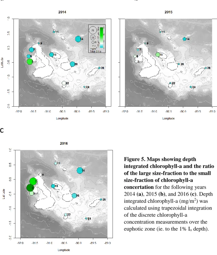
Figure 5. Maps showing depth integrated chlorophyll-a and the ratio of the large size-fraction to the small size-fraction of chlorophyll-a concertation ... 24
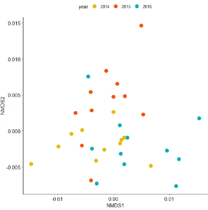
Figure 6. Nonmetric multidimensional scaling (NMDS) of the discrete chemical and biological measurements ... 26
Figure 7. Nonmetric multidimensional scaling (NMDS) of the physical measurements ... 27
Figure 8. Community composition (18S) and biomass. ... 30
Figure 9. Principal component plots of microeukaryote communities ... 32
Figure 10. Maps of deep layer potential density ... 34
Figure 11. Community composition of the Class Alveolata. ... 36
Figure 12. Principal component plots of Alveolata ... 38
Figure 13. Community composition of the Class Stramenopiles. ... 41
Figure 14. Principal component plots of Stramenopiles. ... 43
xi
LIST OF ABBREVIATIONS
18S 18S rDNA
bp base pairs
Chl-a Chlorophyll-a
CTD Conductivity-Temperature-Depth
DI Deionized
DIC Dissolved inorganic carbon EF Equatorial front
ENSO El Niño Southern Oscillation ESW Equatorial surface water EUC Equatorial Undercurrent GMR Galápagos Marine Reserve GNP Galápagos National Park HNLC High nutrient, low chlorophyll-a ITCZ Intertropical convergence zone NECC North equatorial countercurrent OTU Operational taxonomic unit PC Particulate carbon
PCU Peruvian coastal upwelling PN Particulate nitrogen
POC Particulate organic carbon
Rb Raw fluorescence
xii STUW Subtropical underwater
xiii
LIST OF SYMBOLS
Io Incident irradiance at the 50% light level
1
INTRODUCTION
The Galápagos Islands (1-2 °S, 90-92 °W) are volcanically active and began forming five million years ago on the equator, roughly 1000 km west of mainland Ecuador. The islands are famous for having varied habitats which have elicited high biodiversity, especially noted in the macrofauna by naturalists such as Charles Darwin, Barbara and Peter Grant, and others. This holds true in the marine realm, particularly because many major currents converge on the islands, making them a primary productivity hot spot amongst a vast high-nutrient, low-chlorophyll-a (HNLC) region. These currents contribute to the mixing of tropical and subtropical water masses, as well as to the upwelling of nutrients from the Galápagos platform (Fiedler & Talley, 2006; Palacios, 2004a).Various types of topographically induced upwelling stimulate
phytoplankton growth, providing an organic carbon source which supports the islands’ marine food webs. Despite the important ecological role that marine microeukaryotes fill, there are few studies which have addressed them in the Galápagos Islands, especially in assessing how they respond to ecological perturbation.
2
Certain currents are key in influencing the mixing of regional water masses, including the South Equatorial Current (SEC), the North Equatorial Countercurrent (NECC), and the
equatorial undercurrent (EUC). The SEC spans 5 °N-13 °S and 90-140 °W and extends from the surface to ~100 m deep. It flows westward on either side of the equator and interacts with the entire Galápagos platform from east to west. The eastern section of the SEC is cooled by water from the Peruvian Coastal Upwelling (PCU) and the equatorial upwelling. The SEC therefore resembles water mass properties that are intermediate of the equatorial upwelling and the South Pacific subtropical gyre (Pennington et al., 2006). Overlapping with the range of the SEC, the NECC spans 3-9 °N and 91-140 °W and extends from the surface to 100 m deep. It flows
eastward, north of the SEC and transports warm water from the western Pacific warm pool to the east tropical Pacific. The region in which the SEC and the NECC interact (which can be between 2-5 °N) is called the equatorial front (EF). Temperature differences along the EF can cause tropical instability waves (Pennington et al., 2006; Strutton et al., 2008), a sub-seasonal physical perturbation which can occur in addition to the semi-decadal ENSO. The EUC (2°N - 2°S) runs subsurface to the SEC and flows from the western to the eastern boundary upwelling onto the western side of the Galápagos platform (Kessler, 2006). The EUC delivers subtropical
underwater (STUW) located at ~100 m depth to the surface. The STUW is formed from waters of the North and South Pacific subtropical gyres, which are saltier than surrounding water masses, and are well ventilated (Fiedler & Talley, 2006).
3
equatorial cold tongue is less susceptible to temporal variability. Surface properties of the cold tongue are that of the ESW, which have cool, moderately saline water and a shallow but weak pycnocline. The ESW is comprised of water from both the PCU and the equatorial upwelling, which occur seasonally (Fiedler & Talley, 2006). The cold tongue is coldest in September and October, during our sampling period. It usually undergoes seasonal variability of ±1-3 °C. The western side of the Galápagos platform is a temperature minima within the cold tongue, due to the upwelling of the EUC (Fiedler & Talley, 2006).
The physical oceanography of this region is quite complex, making understanding the mechanisms that drive primary production challenging. Moreover, these dynamics are
understudied in local regions such as the coastal waters of the Galápagos Islands. Recently, a group of scientists heavily involved in conservation efforts in the Galápagos Islands met to collaboratively derive an environmental research agenda for the region. They identified 50 questions that were most timely to consider, and of those 7 were within the field of
oceanography. An important outcome was to try to better understand how ENSO influences trophic chains in marine and terrestrial communities (Izurieta et al., 2018).During ENSO equatorial waters warm and weaker trade winds slow the SEC, therefore upwelling is not as prevalent due to the weakening of the EUC.
4
variability in dinoflagellate diversity, which they attributed to be due to the relative availability of water masses sourced from the EUC (Carnicer et al., 2019).
Studies have shown that lapses in upwelling, whether they be from ENSO, seasonal variation, or the discrepancies of local bathymetries, affect phytoplankton biomass throughout the islands (Carnicer et al., 2019; Liu et al., 2014; Schaeffer et al., 2008a; Sweet et al., 2007b). There has been one previous study, a PhD dissertation, that identifies phytoplankton groups found in the Galápagos Islands over an El Niño period. They found that during El Niño the relative abundance of diatoms and chlorophytes decreased, while cyanobacteria and haptophytes increased (McCulloch et al., 2011).
Here we elucidate phytoplankton communities to the genera level using metabarcoding techniques via targeting the 18S rDNA (18S) gene. Identifying to the genera level is helpful when trying to understand the functional diversity of marine microeukaryotes and to posit their unique ecological roles. Without this type of baseline data, it is impossible to know if marine microeukaryotes, typical of the Galápagos Islands, are resistant to perturbations such as ENSO or if their ranges change with climate change (Allison & Martiny, 2008). Other countries have imposed routine monitoring of marine microeukaryotes using 18S and here we share the first of these measurements in the Galápagos Islands (Brown et al., 2018).
This baseline information would complement and extend our current understanding of how ENSO affects this region from both biogeochemical and ecological standpoints. There were three main objectives, separated into 2 parts:
Part 1.
5
2) To examine if these physical conditions could be used to predict chemical and biological measurements.
Part 2.
3) To identify microeukaryote communities in the Galápagos Islands and how they may change from an El Niño (2015) to a normal period (2016).
6
METHODS
Study Region and Sample Collection
Physical, chemical, and biological measurements were taken from various sites (Figure 1) surrounding the Galápagos Islands (89 – 92 ºW, 1.5 ºS – 2 ºN). Sample collection occurred over 15 days in October and reoccurred annually for three years (2014 – 2016) using Galápagos National Park (GNP) monitoring vessels: the M/V Guadalupe River (2014) and the M/V Sierra Negra (2015 and 2016). Based on the Oceanic Niño Index (ONI), periods of El Niño and La Niña within an ENSO occur when the three month running mean of SST is 0.5ºC above or below the threshold for five consecutive months in the Niño 3.4 index (170 – 120 ºW, 5 ºS – 5 ºN). According to the ONI, 2014 was not an anomalous year, 2015 was the strongest El Niño to have occurred since 1950, peaking in December, and 2016 reached the five-month consecutive anomaly period by November, classifying it as a La Niña. The Galápagos Islands however, straddle the Niño 1.2 index (80 – 90 ºW, 0 – 10 ºS) and the Niño 3 index (150 – 90 ºW, 5 – 5 ºS). These indices also were classified as an El Niño in 2015, but in 2016 did not trend to La Niña at a fast-enough rate to be classified as such. Therefore, while we recognize the differences
between 2014 and 2016, for the purposes of this study we will refer to them both as normal years.
At each site a Seabird 19Plus Conductivity-Temperature-Depth (CTD) instrument, equipped with temperature, salinity, fluorescence (FLNTU, WET Labs Inc.), and
7
and 1%, which were calculated from the CTD casts. Depths for discrete samples were
approximate due to some wire angle that occurred during the casts, a product of strong currents. Some sites were only sampled at the surface, in which case water was collected at 10 m depth. Ten L Niskin bottles were used to collect seawater which was then dispensed into acid-cleaned, seawater rinsed 10 L Cubitainers (Hedwin Corporation, Newark, DE, USA) for each Io depth.
8
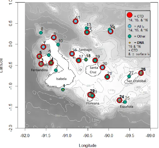
Figure 1. Map of sites sampled during 2014-2016 surveys. Atminimum, if a site was sampled on a given year, a CTD cast was taken. Red indicates that sites have CTD casts performed for every sampling year, and therefore also denote all sites that were sampled in 2014. Additional sites were added in 2015 and 2016. Blue indicates sites in which discrete chemical and biological measurements were collected at all incident irradiance depths (50%, 30%, 10%, and 1%), for all three sampling years. Green indicates ‘other’ sites, in which data gaps vary. For example, some ‘other’ sites may be those in which the surface (10 m depth) was sampled exclusively, while others may only have CTD casts for 2015 and 2016, etc. Orange with a bolded site number indicates sites which have DNA (18S) samples. Some sites sampled for DNA have all Io depths
sampled, while others have only the surface depth sampled, indicated by the blue or green, respectively. Coordinates for site locations can be found in Appendix 5.
Isabela
Santa Cruz Fernandina
Floreana
Española
9 Chlorophyll-a
Field
Chl-a concentrations were used as a biomass proxy for phytoplankton. Size-fractioned chl-a was measured by gravity filtering 400 ml of seawater through Isopore polycarbonate 5 µm filters (47 mm) to obtain the large cell size fraction (> 5 µm). The filtrate was then filtered onto a Whatman GF/F filter (25mm) using an in-line vacuum (< 100 mmHg) to obtain the small cell size fraction (≤ 5 µm). Filters were rinsed with particle-free (0.2 µm filtered) seawater and stored at -20 ºC until onshore analysis. Measurements were taken in triplicate, per irradiance depth, yielding 12 bottles per full site, or three bottles per surface-only site.
Laboratory
Extraction of chl-a samples was performed in the dark. Prior to extraction, samples were placed on ice and incubated for 10 minutes. New 25 ml scintillation vials were rinsed with 90% acetone. Filters were placed in the scintillation vials and 6 ml of 90% acetone was added. Once in acetone, polycarbonate filters were vortexed for 10 seconds while GF/F filters were not. The vials were then stored in the dark at -20 ºC for 24 hours. After this period, the raw fluorescence (Rb) of the chl-a extracts were measured on a Turner Designs 10-AU fluorometer as according to Brand et al. (1981).
Particulate Nutrients and Nutrient Uptake Rates Field
Measurements of particulate nitrogen (PN) and particulate carbon (PC), both plankton biomass proxies, were obtained simultaneously with uptake rates of nitrate and dissolved
10
sea surface temperatures via a flow-through system were covered with screening to mimic different irradiance depths. Triplicate polycarbonate bottles (618 ml) were filled with seawater from each irradiance depth and placed in the respective screened incubation tanks for 24 hrs, beginning in the morning between 6:00 and 8:00 in order to capture the photosynthesis and respiration cycles appropriately. Tracer isotope additions of ≤ 10% of the ambient nutrient
concentrations were used to measure nutrient uptake rates following methods described in Barber et al. (1996). Ambient nitrate and bicarbonate were assumed to be 5 µM and 1200 µM,
respectively. Nitrite concentration was assumed to be < 5% of ambient N, therefore N uptake rates were assumed to be that of nitrate. Nitrate uptake was measured by adding 0.5 µM 15NO3 to
each bottle prior to incubation. Dissolved inorganic carbon (DIC) uptake rates, or net community particulate organic carbon (POC) was measured by adding 120 µM 13C-HCO3 to each bottle prior
to incubation. These incubations were performed in triplicate, per irradiance depth, yielding 12 bottles per full site, or 3 bottles per surface-only site. After incubation, the bottle contents were filtered to capture the plankton community at 24 hrs of exposure to the trace isotopes. The large size fraction (> 5 µm) was filtered onto a 5 µm polycarbonate filter (47 mm) and the filtrate was then filtered onto a pre-combusted (450 ºC for 5 hours) GF/F (25 mm) to obtain the small size fraction (≤ 5 µm). The polycarbonate filter which used to collect the large size fraction was rinsed with particle-free seawater onto a separate pre-combusted GF/F. All filters were stored in petri dishes and frozen at -20 ºC until onshore analysis.
Laboratory
11
prior to use. The pellets were kept in the 96 well plates and stored in a desiccator. Samples were sent to the stable isotope facility at University of California Davis for mass spectrometry
analysis. Ratios of ‘normal’ N and C relative to 15N and 13C concentrations on the filters were used to calculate N-uptake and DIC-uptake rates of the community, as well as the PN and PC present in each bottle.
Dissolved Nutrients
Dissolved nutrients, nitrate, phosphate, and silicate were measured by filtering 30 ml of water through a 0.2 µm filter, using polypropylene FalconTM tube syringes. Between each use, Swivex syringes, including o-rings were acid washed in 10% HCl and rinsed in DI water before air drying. The filtrate was stored at -20 ºC and sent to the stable isotope facility at University of California Davis for mass spectrometry analysis. Nutrient samples were taken in duplicate at each Io depth or at surface-only sites.
DNA for 18S rRNA Analysis Field
Four liters of water from each irradiance depth or surface depth was filtered using an in-line vacuum (< 100 mmHg) through Pall 0.45 µm membrane filters (47 mm). Filters were stored at -20 ºC until onshore analysis.
Laboratory
12
CA, USA). Extracts were diluted either 1:10 or 1:100 so that the starting DNA concentrations were between 20-50 ng/µl. The V4 hypervariable region of the 18S rRNA gene (600 bp) was targeted and amplified using a two-step PCR process (Quigley et al., 2014). All primers used in the first PCR shared the same linker sequence so that barcodes containing illumina specific adapters could be attached during the second PCR. The linker primers contained a section of degenerative nucleotide bases designed to increase the complexity of the library as more iterations of PCR were applied to the sample extracts. These could be used to aid in removing PCR duplicates, although this was not performed in this study. The forward linker primer was 5’- TCG TCG GCA GCG TC + A GAT GTG TAT AAG AGA CAG + NNNN +
CCAGCASCYGCGGTAATTCC -3’, and the reverse linker primer was 5’- GTC TCG TGG GCT CGG + AGA TGT GTA TAA GAG ACAG + NNNN + ACTTTCGTTCTTGAT -3’. The underlined nucleotide bases are the linker sequences, the italicized bases are spacer sequences, the N’s are the degenerative bases, and the bold bases are the v4-18S eukaryotic target
sequences. The linker primers were attached with Illumina forward and reverse barcodes and adapters.
The reagents used for the first PCR included 15 µl Milli-Q water, 2.4 µl ExTaq buffer, 1 µl of forward linker primer, 1 µl of reverse linker primer, 1 µl of ExTaq dNTPs, and 0.125 µl of ExTaq enzymes (Takara Bio Inc., Katsastu, Japan). 5 µl of diluted DNA extract was added to the reaction mixture. Samples were run in the thermocycler at 95 ºC for 5 min, 30 cycles at 95 ºC for 40 s, 59 ºC for 2 min, and 72 ºC for 1 min, followed by a third stage at 72 ºC for 7 min. Products of the reaction were checked on a 1% agarose gel. Products were cleaned using the Qiagen Qiaquick PCR purification kit (Qiagen, Germantown, MD, USA) and
13
same assay kit previously mentioned. The reagents used for the second PCR included 9.5 µl Milli-Q water, 3 µl of barcoded forward primer, 3 µl of barcoded reverse primer, 2 µl ExTaq buffer, 0.5 µl of ExTaq dNTPs, and 0.1 µl of ExTaq enzyme. Two µl of PCR product from the first reaction, diluted to 10 ng/µl was added to the reaction mixture. Samples were run in the thermocycler at 95 ºC for 5 min, 4-10 cycles at 95 ºC for 40 s, 59 ºC for 2 min, and 72 ºC for 1 min, followed by a third stage at 72 ºC for 7 min. Samples were checked on a 1% agarose gel every 2 cycles until faint bands were achieved. Products were excised from the gel and cleaned using the Qiagen Gel Extraction kit (Qiagen, Germantown, MD, USA) and manufacturer
provided protocol. DNA concentrations of the products were quantified and samples were pooled so that each sample was represented at a concentration of 10 ng/µl. The pool was run in a single large gel lane on a 1% SYBR Green (Invitrogen, Carlsbad, CA, USA) stained gel. The target band was excised and weighed. It was then divided into parts that weighed < 400 mg, the maximum weight recommended by the manufacturer per reaction chamber of Qiagen Gel Extraction kits (Qiagen, Germantown, MD, USA). Each part was cleaned with the Qiagen Gel Extraction kit. The products from the kit were pooled back together and the library was
submitted for sequencing to the University of North Carolina at Chapel Hill High Throughput Sequencing Facility across two lanes of Illumina MiSeq (2 × 300).
Amplicon assembly and Quality Control
14
control, merging, and removing chimeras (Appendix 1). Rarefaction and additional sample cleaning steps were performed in R v. 3.5.3 using the phyloseq v. 1. 24. 2 and vegan v. 2.5-4 packages. Mean amplicon length for sequencing lane 1 was 561 bp, while mean amplicon length for sequencing lane 2 was 599 bp. Multiplexed sequence files were in the CASAVA 1.8 FASTQ format and were demultiplexed using QIIME 2. Denoising was done using the QIIME 2 plug-in DADA2, in which reverse reads and forward reads from lane 2 were truncated to 260 bp and 280 bp, respectively, while the reverse reads and forward reads from lane 1 were truncated to 250 bp and 210 bp, respectively. Chimeras were removed by the consensus method and reads were merged. Assembled amplicons were annotated by blasting to the SILVA v. 123 reference database using a 90% pairwise identity cutoff. Metazoans were removed. Technical replicates were pooled, as they all met expected similarity thresholds (Wen et al 2017). Of the 61 samples, 41 were technical replicates. Those 41 were pooled to represent 19 samples; the total samples now being 39. These samples were rarefied to 2066 reads. Six samples were removed due to rarefication, yielding 33 annotated samples represented by 1002 OTUs. From the remaining samples, sites were chosen if they had samples for both 2015 and 2016. Sixteen of the 33
samples, or 8 sites, met these criteria and comprised of the sample sites 1, 3, 4, 5, 18, 22, 24, and 26 (Appendix 2). Rarefaction curves are displayed in Appendix 3. Custom taxonomies
(Appendix 4) were assigned in certain cases, described in the following section.
Data Preparation and Statistical Analysis Physical Measurements
15
using the sw_pden() function from the Mixing (MX) Oceanographic toolbox v 1.8.0.0 in MATLAB (R2017b). The mixed layer depth was defined as the depth in which the change in potential density (Δρθ) from the surface was > 0.35 kg/m3. The depth at which the deep layer
began was determined by calculating when the density from the bottom of the cast differed from the density at a shallower depth by > 0.2 kg/m3. This marked the top of the deep layer or the deep layer depth. These density cut-off values were chosen based on the visual inspection of all CTD casts and defined the layers appropriately. The remaining area between the mixed layer depth and the deep layer depth was the intermediate layer. Temperature, salinity, and potential density of the mixed and deep layers were averaged from CTD cast measurements. Δρθ over the
intermediate layer was calculated as the difference in potential density averages of the deep and mixed layers. These calculations are displayed in Appendix 5.
Discrete Chemical and Biological Measurements
Discrete chemical and biological measurements are displayed in Appendix 6 and flow cytometry measurements are displayed in Appendix 7. Chl-a, PN, and PC were all measured to use as proxies for plankton biomass. At full sites (ie. all incident irradiance depths sampled), select chemical and biological measurements were depth integrated using trapezoidal integration (Appendix 8). These full sites included: 3, 5, 7, 9, 11, 14, 16, 20, 22, 24, and 26.
Size-fractionated measurements of chl-a as well as PN and PC were used to consider the ratio of large phytoplankton cells (> 5 µm) to small phytoplankton cells (≤ 5 µm). F-ratio, a proxy for the ratio of new production to total production, was calculated using methods from Aufdenkampe et al., (2002).
16
certain chemical and biological parameters. Sites that met these criteria included: 3, 5, 7, 9, 11, 12, 14, 16, 22, 24, and 26. Spearman’s ρ correlations were used to assess relationships between dissolved nutrients and the physical properties of the different layers. Kruskal-Wallis tests were used to see how uptake rates and f-ratios varied between years. The R package Vegan_2 5.4 was used to perform an unconstrained direct gradient analysis by calculating Bray-Curtis
dissimilarity matrices for the physical measurements as well as the chemical, biological, and flow cytometry measurements, separately. A two-way PERMANOVA (Vegan function ‘adonis’) test was performed on each matrix to see if samples varied more by site or over sampling
timepoints. A Mantel’s test (Vegan function mantel) was then used to see if the dissimilarities between the sample physical measurements correlated to the dissimilarities between the sample chemical, biological, and flow cytometry measurements. Bray-Curtis dissimilarity matrices were visualized on non-metric multidimensional scaling (NMDS) plots.
Amplicons
17
2132 OTUs at the genera level that consisted of Archaea, Bacteria, and Eukaryotes. At the site sampled within a comparable region to our sample sites, Eukaryotes made up ~10% of the relative abundance (Rojas-jiméne, 2018). While the exact number of OTUs was not evident in the study, I estimated that they had ~210 genera of eukaryotes. We had ~120 genera of
eukaryotes, prior to grouping unknown and uncultured OTUs (Appendix 2).
The OTU table was then transformed using a Hellinger’s transformation by taking the square root of the relative proportions of OTUs at the genus level. This transformation places less weight on OTUs with a high relative proportion, which was appropriate given that the majority of OTUs represented low proportions of the samples. A dissimilarity matrix was then calculated based on eigenvalues (base R function princomp) which preforms principle
18
RESULTS
Part 1.
One effort of our study was to gain an understanding of the physical oceanographic make-up of the sampled region, and how it may change from a normal period (2014) through an El Niño (2015) to another normal period (2016). Part of the motivation for this was to determine if physical changes correlated with changes in chemical and biological measurements.
Physical oceanographic conditions
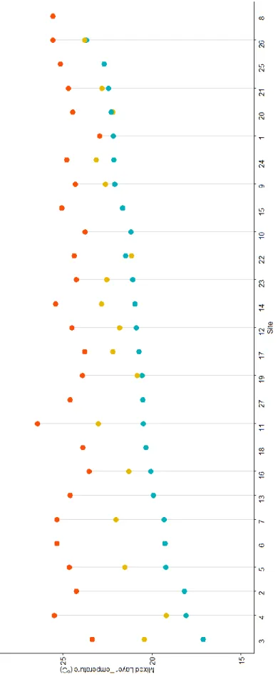
Average mixed layer temperature showed distinct changes over the three years (Figure 2). The coolest mixed layer temperatures at all sites were observed in 2016, except for sites 22 and 20, which were marginally cooler in 2014. Sites 2 through 7, located to the west of islands Isabela and Fernandina had the coolest mixed layers, an indication of the EUC upwelling. This pattern only remained consistent in 2016 and at site 4 in 2014. Sites 3, 5, and 7 were comparable temperatures to other mixed layer measurements during 2014 and sites 2 and 6 were not
19 F igu re 2. Ave rag e m ixe d layer te m p er ature s ca lcul ate d f rom CTD c as ts. S it es orde re
d in i
20 Chemical and biological conditions
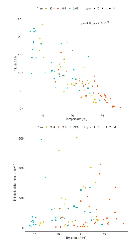
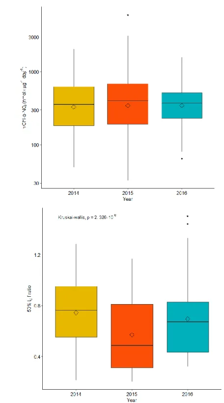
Seawater temperature across the mixed, intermediate, and deep layers showed a significant negative relationship (ρ = -0.85, p = 2.2e-16) with dissolved nitrate concentrations (Figure 3a), implying that higher nitrate concentrations are associated with cooler waters, often at depth. However, temperature did not have a relationship with nitrate uptake rates (Figure 3b), indicating that nitrate demand was not a function of just temperature and that nitrate may be biologically available irrespective of changes in temperature and the physical conditions which those changes imply. Biomass (chl-a) normalized nitrate uptake rates (VChl-a-NO3) did not
change significantly between years (Figure 4a), but new production relative to the total
21
a
b
22
a
b
Figure 4. Box plots of biomass normalized nitrate uptake and 50% Io f-ratio.(a) Box plots showing the median, mean, and interquartile range of VChl-a-NO3 for all years (2014-2016). (b)
Box plots showing the median, mean, and interquartile range of the 50% Io f-ratiofor all years
23
24
a
b
c
Figure 5. Maps showing depth
integrated chlorophyll-a and the ratio of the large size-fraction to the small size-fraction of chlorophyll-a
concertation for the following years 2014 (a), 2015 (b), and 2016 (c). Depth integrated chlorophyll-a (mg/m2) was calculated using trapezoidal integration of the discrete chlorophyll-a
25
The differences in chemical, biological, and flow cytometry measurements between the three years were more site specific (R2 = 0.20, p < 0.001) than they were year specific, however groupings were not strong, indicating the high variability chemically and biologically throughout the Galápagos Islands (Figure 6). The physical conditions differed more temporally than they did spatially (R2 = 0.11, p = 0.028) (Figure 7). Additionally, the physical conditions at the sites did
not correlate to the differences in chemical, biological, and flow cytometry at the sites (Mantel statistic r: 0.1252, p = 0.128).
26
27
Figure 7. Nonmetric multidimensional scaling (NMDS) of the physical measurements: deep layer depth, mixed layer depth, potential density of the deep layer, potential density of the mixed layer, salinity of the deep layer, salinity of the mixed layer, temperature of the deep layer,
temperature of the mixed layer, thickness of the intermediate layer, and change in density over the intermediate layer for all sites based on Bray-Curtis dissimilarity. Differences between samples could be explained more by sampling year than by site.
28 Part 2.
Another motivation of our study was to identify microeukaryote communities that can be observed in the Galápagos Islands. Additionally, we sought to see if there was variability in community composition spatially and temporally.
Microeukaryote Plankton Composition
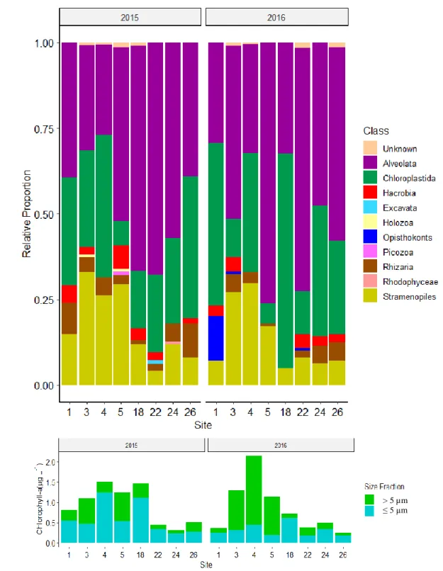
The microeukaryote plankton were represented by 10 major class levels or equivalent groups: Alveolata, Chloroplastida, Hacrobia, Excavata, Holozoa, Opisthokonts, Picozoa, Rhizaria, Rhodophyceae, and Stramenopiles (Figure 8a). The three most abundant groups, the Alveolata, Chloroplastida, and Stramenopiles, were present at all sites in 2015 and 2016. Either the Alveolata or the Chloroplastida were the classes with the highest relative proportion. In 2015, Alveolata had the largest relative proportion in samples 5, 18, 22, and 24, while Chloroplastida had the largest relative proportion at the remaining sites. In 2016, Alveolata had the largest relative proportion at sites 3, 5, and 22, while Chloroplastida had the largest relative proportion at the remaining sites. Stramenopiles conserved relative proportion trends across both years, having the highest proportions at sites 3, 4, and 5. Despite the similarity in relative proportions, it’s important to note the differences in biomass between the years (Figure 8b). Moreover, a caveat of using chl-a concentrations to view the relative proportion plots in a ‘biomass normalized’ manner is that not all plankton sequenced would have contained chl-a.
29
in 2016, and were especially abundant at site 1, where they made up the third largest proportion of that community. The Opisthokonts were filtered of Metazoans, and therefore consisted of fungi. Additionally, Opisthokonts were also present at sites 3 and 22. Holozoans, Picozoans, Excavata, and Rhodophyceae were only present in 2015. Holozoans were present at sites 3 and 5. The Picozoans, Excavata, and Rhodophyceae which were present at sites 5, 22, and 24,
respectively.
At these coarse class group levels, changes in relative abundance occurred from 2015 to 2016. Stramenopiles decreased at all sites except 4 and 22. At site 18, Chloroplastida increased to be in majority in 2016 at the expense of Alveolata and Stramenopile proportions observed in 2015. At site 5, the Alveolata increased at the expense of the Stramenopiles and other less
30
a
b
Figure 8. Community composition (18S) and biomass.(a) Relative proportions of
microeukaryotes at class level groupings for 2015 and 2016. (b) Stacked bar chart showing the proportion of large cell size-fractioned chlorophyll-a to small cell size-fractioned chlorophyll-a and total chlorophyll-a concentrations at each site. Note that the 18S samples comprise of plankton > 0.45 µm.
31
32
a
b
c
33
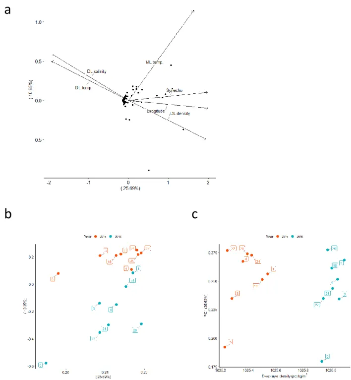
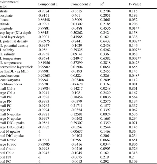
Table 1. Correlation coefficients and significance of environmental factors correlated to the differences between microeukaryote communities at the genera level. Output of the envfit function, a function from the R package Vegan that fits environmental factors onto ordinations. Environmental factors are from flow cytometry measurements and the discrete chemical and biological measurements. Significant environmental factors are displayed as vectors on Figure 9a.
Environmental
Factor Component 1 Component 2 R
2 P-Value
Nitrate -0.9324 -0.3615 0.2704 0.115
Phosphate -0.9161 -0.401 0.2051 0.193
Silicate 0.86548 -0.5009 0.3661 0.052
Latitude -0.9995 0.03302 0.2185 0.206
Longitude 0.99881 -0.0488 0.4536 0.014*
Deep layer (DL) depth 0.86451 0.50262 0.2424 0.158
Mixed layer depth -0.9001 0.43565 0.162 0.338
DL potential density 0.96975 -0.2441 0.6432 0.002**
ML potential density -0.9947 -0.1029 0.2458 0.146
DL salinity -0.956 0.29325 0.5262 0.007**
ML salinity -0.9958 0.09141 0.336 0.058
DL temperature -0.9684 0.24947 0.6382 0.002**
ML temperature 0.81956 0.57299 0.3818 0.042*
Intermediate layer thick 0.99982 0.01904 0.0651 0.655
Δρθ (|ρθ DL - ρθ ML|) 0.99981 -0.0193 0.2455 0.145
Synechococcus 0.99863 0.05224 0.3864 0.048*
Picoeukaryotes 0.9994 -0.03466 0.2805 0.112
Prochlorococcus 0.9978 0.06628 0.3162 0.081
Small Chl-a 0.98984 0.14217 0.0248 0.861
Large Chl-a -0.9941 -0.1081 0.2429 0.167
Small PN -0.9828 0.18454 0.0836 0.564
Large PN -0.9993 -0.0379 0.2576 0.134
Small PC -0.9762 0.21711 0.1577 0.337
Large PC -0.9994 -0.0354 0.3397 0.067
Small N-uptake -0.9921 0.12581 0.0924 0.536
Large N-uptake -0.9997 -0.0262 0.1665 0.294
Small DIC-uptake -0.9561 0.29307 0.3359 0.071
Large DIC-uptake -0.9982 -0.0596 0.2544 0.145
Total N-uptake -1 0.00637 0.1468 0.36
Total DIC-uptake -1 -0.0103 0.2064 0.234
Small f-ratio -0.9997 0.0256 0.0662 0.651
Large f-ratio 0.93985 -0.3416 0.0344 0.806
Total f-ratio -0.9998 -0.0216 0.0905 0.526
Total Chl-a -0.9945 -0.1045 0.162 0.318
Total PN -1 -0.0075 0.219 0.2
Total PC -1 -0.0013 0.292 0.109
34
a
b
c
Figure 10. Maps of deep layer potential density 2014 (a), 2015 (b), and 2016 (c)
35 Aveolata Composition
The Alveolata consist of four major groups of eukaryotic plankton: the alveolates, apicomplexans, ciliates, and dinoflagellates (Figure 11). Of the Alveolata, there were 34 genera represented across the sampled sites. In 2015, two alveolate groups, Syndiniales Group I and Syndiniales Group II, were present and represented the largest relative proportion at all of the sites. Both Syndiniales I and Syndiniales II remained present in 2016 at sites 1, 3, 4, 22, 24, and 26. Site 22 had the highest relative proportion of Alveolata in 2015 and had the highest relative proportion of Syndiniales Group II of all sites irrespective of year. In 2016 at site 18, Syndiniales I was present without the presence of Synidiniales II, which is the only instance of this.
Another dominant group that was generally associated with Syndiniales I and II was Syndiniales III. Syndiniales III was present in 2015 at stations 3, 4, 5, 18, 24, and 26; while in 2016, it was present at stations 1 and 24. The most obvious difference between sites from 2015 to 2016 is the reduction of Syndiniales I and II as well as the dominance of the dinoflagellate Gyrodinium in 2016. Gyrodinium was found at site 5 in 2015, as well as sites 3, 4, 5, 22, 24, and 26 in 2016, making up a large portion of the Alveolata in the 2016 samples.
36
22 and 24 in 2016, but took up a large proportion at those sites. Interestingly, there were more unknown (unable to match to a reference sequence in the database) Alveolata in 2016.
Figure 11. Community composition of the Class Alveolata. Relative proportions of Alveolata at the genus level for 2015 and 2016.
37
significant correlate by a fair margin was the longitude of site location (R2 = 0.70, p < 0.001),
suggesting that the changes in alveolates were more affected spatially than differences between the years, relative to the whole microeukaryote community. When site loadings for principle component 1 were plotted verses longitude the relationship was statistically significant (ρ = 0.674, p = 0.0042) and the sites did not separate by year. Similarly, deep layer water properties were correlated with the differences amongst the Alveolata community. These, in order of high to low R2 value, included temperature of the deep layer, density of the deep layer, and salinity of the deep layer. Mixed layer salinity also significantly correlated with the differences amongst the Alveolata (R2 = 0.51, p = 0.008). Other correlations with physical measurements included Δρθ of
the intermediate layer, temperature of the mixed layer, and potential density of the mixed layer. Some physiological and biological measurements were correlated with genus level differences in the Alveolata between sites from 2015 to 2016. Prochlorococcus cell counts and the small size-fraction (≤ 5µm) of DIC uptake were strongly correlated (R2 = 0.53, p = 0.008; R2
= 0.47, p = 0.016, respectively) with differences amongst Alveolata communities. When site loadings for principle component 1 were plotted verses longitude the relationship was
38
a
b
c
Figure 12. Principal component plots of Alveolata. (a) PCA plot showing PC1 verses PC2 of Alveolata genera based on eigenvalues. Significant environmental variables that correlated with differences in relative proportions of genera are plotted as vectors. (b) Plot of longitude verses PC1, showing a significant relationship (Spearman, ρ=0.674, p<0.05). (c) Plot of
39
Table 2. Correlation coefficients and significance of environmental factors correlated to the differences between Alveolata communities at the genera level. Output of the envfit function, a function from the R package Vegan, that fits environmental factors onto ordinations.
Environmental factors are from flow cytometry measurements and the discrete chemical and biological measurements. Significant environmental factors are displayed as vectors on Figure 12a.
Environmental
Factor Component 1 Component 2 R
2 P-Value
Nitrate -0.9735 -0.2287 0.3049 0.108
Phosphate -0.982 -0.189 0.2486 0.173
Silicate -0.4812 -0.8766 0.33 0.088
Latitude -0.9931 0.11746 0.3234 0.076
Longitude 0.98705 -0.1604 0.6997 0.001***
Deep layer (DL) depth 0.87214 0.48925 0.2246 0.181
Mixed layer (ML) depth 0.919 0.39426 0.1273 0.421
DL potential density 0.68599 -0.7276 0.5073 0.009**
ML potential density -0.9997 -0.0249 0.3652 0.048*
DL salinity -0.816 0.57803 0.4889 0.013*
ML salinity -0.9731 0.23047 0.505 0.008**
DL temperature -0.7066 0.70763 0.5119 0.009**
ML temperature 0.95525 0.29578 0.4179 0.033*
Intermediate layer thick 0.62532 0.78037 0.0347 0.81
Δρθ (|ρθ DL - ρθ ML|) 0.99401 -0.1093 0.4044 0.035*
Synechococcus 0.99006 0.14068 0.4202 0.024*
Picoeukaryotes 0.99975 -0.0224 0.0874 0.525
Prochlorococcus 0.99991 -0.0133 0.5332 0.008**
Small Chl-a -0.9535 0.30148 0.0922 0.536
Large Chl-a -0.9956 -0.0943 0.3364 0.075
Small PN -0.96 0.28002 0.3306 0.081
Large PN -1 0.00166 0.3687 0.05*
Small PC -0.9461 0.32398 0.3822 0.051
Large PC -1 0.00186 0.4665 0.016*
Small N-uptake -0.9688 0.24773 0.3067 0.097
Large N-uptake -0.9998 0.02049 0.2518 0.169
Small DIC-uptake -0.9066 0.42191 0.4968 0.013*
Large DIC-uptake -0.9993 -0.0376 0.3547 0.061
Total N-uptake -0.9959 0.09024 0.2994 0.111
Total DIC-uptake -0.9984 0.05634 0.3627 0.06
Small f-ratio -0.9904 0.13802 0.1911 0.261
Large f-ratio -0.999 -0.0445 0.0446 0.768
Total f-ratio -0.9968 0.08032 0.1968 0.243
Total Chl-a -0.9999 -0.0163 0.3042 0.095
Total PN -0.9972 0.07509 0.4303 0.032*
Total PC -0.997 0.07718 0.5224 0.008**
40 Stramenopile Composition
The Stramenopiles consist of oomycetes, brown algae, and the Bracillariophyceae (diatoms). Of the Stramenopiles, there were 22 genera represented across the sampled sites (Figure 13). Sites 3, 4, and 5 had the highest total relative proportion of Stramenopiles
41
Figure 13. Community composition of the Class Stramenopiles. Relative proportions of Stramenopiles at the genera level for 2015 and 2016.
We used principal component analysis to identify within the Stramenopiles if there were significant differences in Stramenopiles genera between sites from 2015 to 2016 (Figure 14). The strongest environmental correlates (Table 3) with Stramenopile community differences were density and temperature of the deep layer (R2 = 0.65, p < 0.001; R2 = 0.64, p < 0.001,
respectively). Other physical conditions with significant correlations, in order from highest R2,
42
differences in the Stramenopiles between sites from 2015 to 2016 (Table 3). Synechococcus and Prochlorochoccus counts strongly correlated (R2 = 0.64, p = 0.003; R2 = 0.60, p = 0.004,
43
a
b
c
44
Table 3. Correlation coefficients and significance of environmental factors correlated to the differences between Stramenopile communities at the genera level. Output of the envfit function, a function from the R package Vegan that fits environmental factors onto ordinations. Environmental factors are from flow cytometry measurements and the discrete chemical and biological measurements. Significant environmental factors are displayed as vectors on Figure 14a.
Environmental
Factor Component 1 Component 2 R
2 P-Value
Nitrate -1 -0.0075 0.3227 0.1
Phosphate -0.9999 0.01412 0.2816 0.132
Silicate -0.9945 -0.105 0.2737 0.153
Latitude -0.9986 0.05272 0.247 0.16
Longitude 0.98485 -0.1734 0.462 0.024*
Deep layer (DL) depth 0.99993 0.01153 0.2243 0.222
Mixed layer depth 0.96642 0.25697 0.2023 0.249
DL potential density -0.8829 -0.4696 0.6527 0.001***
ML potential density -0.9992 -0.0403 0.3934 0.049*
DL salinity 0.83584 0.54897 0.4968 0.012*
ML salinity -0.9077 0.41966 0.2748 0.135
DL temperature 0.87891 0.47698 0.6441 0.001***
ML temperature 0.9911 0.13313 0.4716 0.017*
Intermediate layer thick 0.85634 -0.5164 0.151 0.359
Δρθ (|ρθ DL - ρθ ML|) 0.99074 -0.1358 0.3678 0.058
Synechococcus 0.97394 -0.2268 0.6404 0.003**
Picoeukaryotes 0.81423 -0.5805 0.3577 0.058
Prochlorococcus 0.99519 0.09798 0.6044 0.004**
Small Chl-a -0.7763 -0.6303 0.0458 0.744
Large Chl-a -0.999 0.04468 0.3646 0.057
Small PN -0.9543 -0.2988 0.0538 0.696
Large PN -0.9948 0.10168 0.4157 0.033*
Small PC -0.8357 -0.5492 0.0168 0.896
Large PC -0.9961 0.08879 0.5121 0.013*
Small N-uptake -0.9592 0.28264 0.1107 0.453
Large N-uptake -0.9835 0.18076 0.388 0.054
Small DIC-uptake 0.89395 0.44817 0.0351 0.81
Large DIC-uptake -0.9965 0.08323 0.4081 0.031*
Total N-uptake -0.9811 0.1937 0.4077 0.046*
Total DIC-uptake -0.9941 0.10842 0.3969 0.038*
Small f-ratio -0.9821 0.18864 0.2137 0.232
Large f-ratio -0.9935 -0.1141 0.0742 0.623
Total f-ratio -0.9936 0.11305 0.2414 0.191
Total Chl-a -1 0.00511 0.3274 0.074
Total PN -0.9978 0.06589 0.4046 0.035*
Total PC -0.9977 0.06845 0.4752 0.016*
45 Chlorophyte Composition
46
47
DISCUSSION
Part 1.
The eastern equatorial Pacific Ocean is an HNLC known to have high nitrate and phosphate concentrations, yet chronically low phytoplankton biomass due to iron limitation (Behrenfeld et al., 1996). Understanding these dynamics and what they mean for this region ecologically remain on the forefront of pertinent questions in oceanography. In the waters surrounding the Galápagos Islands, HNLC conditions are generally relieved. This is due in part to the interaction of currents with the islands’ topography, especially the EUC which upwells onto the platform from the west. Additionally, equatorial upwelling, forming the cold tongue, is ever present. Seasonally, the cold tongue is coolest in September and October (Fiedler and Talley 2006), over which period we performed our surveys. The Galápagos Islands follow Southern hemisphere seasonality such that the period from May to November, or Garúa (mist) season, has colder SST. The cooler water and warmer air temperatures during this time of year cause water to condense from the air, increasing the humidity, hence the name, Garúa (Sweet at al 2008). Despite sampling within the same season during the cooler part of the year, we observed an average of ~ 2 ℃ difference in mixed layer temperature between 2015 and 2016. This was due to the ENSO signal, which by definition is a positive anomaly in SST. Because of this, there have been many studies which use SST to try to understand chlorophyll-a dynamics in the eastern equatorial Pacific region (Banks, 2003; G. C. Feldman, 1986; G. Feldman, Clark, & Halpern, 1984; Palacios, 2004b; Schaeffer et al., 2008b; W. V. Sweet et al., 2007a).
48
are also recycled in the mixed layer. The Galápagos Islands are embedded within this region but can benefit from lithogenic sources of iron (Barber & Chavez, 1991; Rafter et al., 2017), due to the currents topographically interacting with the islands. This natural iron enrichment that leads to phytoplankton blooms is a phenomena termed “island mass effect” (Martin et al., 1994; Palacios, 2002). It is caused by any processes which enhance vertical mixing when encountering an island, such as tidal mixing or wind driven coastal and equatorial upwelling (Feldman, 1986). Particular areas in the Galápagos have higher iron availability than others such as Bahía
Elizabeth, a shallow bay on the west side of Isabela (Edgar et al., 2004; Kislik et al., 2017). Its shallow depth results in relatively weak vertical mixing required to resuspend iron. When vertical mixing is adequate, “island mass affect” can occur causing large phytoplankton blooms that eventually deplete nitrate (Martin et al., 1994). Therefore, we suspected that the strength and duration of vertical mixing has a strong control over whether phytoplankton become limited by iron or nitrate, or perhaps undergo co-limitation. We found that nitrate concentration strongly correlated with water temperature and that cooler, deeper water had higher nitrate. This
observation corroborates the idea that vertical mixing is critical for the delivery of all nutrients to the surface waters. Nitrate uptake, or an indication of the rate of new production, did not
correlate with water temperature. This showed that at these local scales, temperature alone is not enough to predict the occurrence of phytoplankton biomass and warrants the need for more fine scale field observations.
49
(Edgar et al., 2004). Previous studies have sought to understand patterns of localized
phytoplankton biomass and how they change seasonally (Palacios, 2002, 2004a). These studies have relied on ocean color derived from satellites and the interpolation of in situ chl-a
measurements to try to understand the seasonality of primary production. The chl-a patterns derived from satellites can best be described by both annual and semi-annual signals. Annually, SST change on a basin scale due to the migration of the intertropical convergence zone (ITCZ). Semi-annually, two modes of physical disturbances are found to explain variation of satellite chl-a pchl-atterns. The strongest of the two wchl-as identified chl-as the migrchl-ation of the EF, where the wchl-arm TSW of the north meet the cool ESW. The other mode identified as critical in controlling chl-a was the upwelling of STUW from the western side of the platform (Palacios, 2002).
Interestingly, past studies have found that this secondary mode is not nearly as critical as the migration of the EF. However, this was only deemed true from observations which lacked the compounding impact of an El Niño.
50
well by the remotely sensed and measured parameters from those studies. In one such study, depth of the thermocline could explain some of the observed chlorophyll-a variability (R2 = 0.21, p > 0.05) and in other studies this has also been identified as an important physical feature for the broader eastern equatorial region, but none of these findings yielded statistical significance (Palacios, 2002; W. V. Sweet et al., 2007a). Similarly, we found that differences in physical conditions amongst the sites could not collectively account for the differences in the chemical, biological and flow cytometry measurements at all sites. The chemical, biological and flow cytometry measurements differed more spatially.
Part 2.
The only other study to our knowledge that has looked specifically at phytoplankton communities in the Galápagos Islands during an El Niño used high-performance liquid chromatography (HPLC) and chemical taxonomy analysis (CHEMTAX), to classify phytoplankton, based on their pigments, by the following groups: diatoms, chrysophytes, chlorophytes, cyanobacteria, and haptophytes (McCulloch et al. unpublished 2011).
51
during El Niño, and the diatoms and pelagophytes in the transition to La Niña (McCulloch et al. unpublished 2011). Haptophytes, which fall under the class Hacrobia, did not comprise of a large proportion in our samples, but were consistently present across sites. We did see that small cell size-fractions (≤ 5µm) contributed more to chl-a concentrations over the El Niño than did large cell size-fractions (> 5µm). Based on our flow cytometry counts and relative proportions of microeukaryote communities, we see that cyanobacteria and dinoflagellates contributed most to chl-a concentrations during the 2015 El Niño, while diatoms and dinoflagellates were the main contributors in 2016.
Dinoflagellates made a larger relative proportion of the phytoplankton communities than we had anticipated, likely due to their diverse life strategies that can allow them to bloom at various stages of the upwelling cycle. Dinoflagellates which are thought to have the best chances of success during upwelling typically are capable of a dormant over-wintering stage (Smayda & Trainer, 2010). We observed large relative proportions of Gyrodinium, which are meroplanktonic and capable of forming germinating resting cysts that can store nutrients for long periods of time whilst remaining in the sediments (Anderson et al., 1985). A previous study in the Galápagos Islands focused on surveying dinoflagellates since many species are harmful algae (Carnicer et al., 2019). They identified 152 taxa and 38 dinoflagellate genera. But despite high species richness, a majority of the abundance making up the dinoflagellate communities were benthic species, that could survive suspended within the water column. These taxa included
Prorocentrum lima, Coolia sp., Ostereopsis cf. lenticularis, and Ostereopsis cf. ovata. Ostereopsis cf. ovata made up 46% of the dinoflagellate abundances (Carnicer et al., 2019).
52
relaxation occurs. For example, if relaxation with in a region commonly occurs on the order of days, than in order for a dinoflagellate to bloom during an upwelling, it may need to be able to form a resting spore capable of supplying it with enough nutrients for it to survive over those relaxation days (Smayda & Trainer, 2010). In this sense, Gyrodinium meets the criteria of a dinoflagellate that would succeed semi-decadal gaps in the upwelling cycle controlled by ENSO. Another adaptation dinoflagellates must have to thrive in upwelling, is the ability to tolerate a range of mixing and advection habitats, defying the traditional Margalef model which proposes that high-nutrient and light, low turbulent conditions are “ideal” for a dinoflagellate bloom (Wyatt, 2014). Blooms of Gyrodinium have been documented as being advected from offshore to their coastal location, surviving strong horizontal shear (Raine et al., 1993). Our observations also challenge the classic stratification-dinoflagellate bloom paradigm (Smayda, 2002), indicated by the importance of deep layer water density in predicting communities which suggests that phytoplankton groups observed should be able to endure entrainment within currents and vertical mixing.
There are other eco-physiological advantages that Gyrodinium sp. have which may also help explain its co-occurrence with diatoms, as well as the inability of diatoms to take up a majority of the relative proportions of the community during the normal year (2016).
53
upwelling (Neuer & Cowles, 1994). Moreover, Gyrodinium sp. have the ability to ingest prey that is as large as its own size via engulfment, as well as other strengths which include the ability to reduce its rate of metabolism when prey availability is low (Hansen, 1992). But perhaps what stopped Gyrodinium sp. from taking up even greater relative proportions is that they have lower growth rates than many of their ciliate competitors (Silva et al., 2009), and we found ciliates to be amongst the observed Alveolata communities.
In upwelling systems, diatom and dinoflagellate blooms commonly occur simultaneously (Smayda & Trainer, 2010). Chaetoceros sp. can form resting spores anticipatory of upwelling relaxation and continuous sporulation as well as rapid germination put it at an advantage
(Smayda, 2002), which may be why we still observe their presence in 2016 despite knowing that they can be grazed on by Gyrodinium sp. In similar fashion to to Gyrodinium sp., Chaetoceros sp. are able to produce both vegetative cells and resting cysts (Pitcher et al., 1991). Chaetoceros sp. are also less susceptible to horizontal advection than other diatoms (Tilstone et al., 2000). It’s possible that due to these advantages, Chaetoceros sp. was able to maintain high relative
proportions from the El Niño to the normal year.
54
Corethron sp. were also present over both years west of Isabela and this was consistent with other studies (McCulloch et al. unpublished 2011). Another defining feature of 2015 was the large relative proportions of the Syndiniales sp. In light of 18S rRNA techniques, parasitism in the ocean, especially that by the Syndiniales sp. is more prevalent than previously recognized (Guillou et al., 2008). To our knowledge, this was the first documentation of their presence in the Galápagos Islands. Dinoflagellates are common hosts to parasitic Syndiniales sp. (Jephcott et al., 2016). The relative proportions of Syndiniales sp. along with other heterotrophic Alveolata could be a cause for lower average f-ratios in 2015, relative to 2014 and 2016.
The Chlorophyta had a constant and consistent presence throughout the DNA sample sites. Worldwide, Chlorophyta are ubiquitous, commonly found in the coastal ocean, especially in oligotrophic regions (Tragin & Vaulot, 2018). Ostreococcus sp. other than Subclades A and B, where the most common Chlorophyta genus identified. Ostreococcus sp. is the smallest known photosynthetic eukaryote currently (Tragin et al., 2016). They are typically 0.8 µm (Chrétiennot-Dinet et al. 1995). In the PCU, diatoms and dinoflagellates are common, however
picophytoplankton consistently make up a majority of the microeukaryote communities.
Included in these picophytoplankton are the dominant chlorophyte, Ostereococcus sp.(Rii et al., 2016). We observed similar patterns, perhaps another indicator of the importance in water mass sources in contributing to microeukaryote community composition.
55
importance of understanding the baseline phytoplankton taxa, seasonal differences in microeukaryotes, and overall production of the Galápagos Islands (Carnicer et al., 2019;
56
APPENDIX 1: NO. OF READS PER SAMPLE AFTER VARIOUS BIOINFORMATIC STEPS Appendix 1. Table of original sample ID’s (note that nomenclature varies due to separate
sampling runs on Illumina, indicated by the Illumina lane value). Sequenced samples were mainly from incident irradiance (Io) depth 1 (50%) but some are from depths 2 or 3, 30% or 10%,
respectively. Reads show the number that were put into QIIME II, retained after filtering,
denoised in DADA-2, merged, and had chimeras removed. Three samples were lost during these steps, resulting in the 61 samples listed in this table. Bolded sample ID’s were used for 18S analysis and were pooled if considered technical replicates.
Sample ID Illumina Lane
Site Year Io Depth
Level
Reads
input filtered denoised merged non-chimeric
G15-1-1 1 1 ‘15 1 33767 20362 20362 9377 9241
1_1_2015 2 ‘15 1 26560 7555 7555 3781 1335
1_1_2016 2 ‘16 1 191084 152385 152385 130136 28722
G15-2-1 1 2 ‘15 1 45392 19004 19004 11365 11365
2_1_2015 2 ‘15 1 45305 38655 38655 25928 12833
G14-1-1 1 3 ‘14 1 14789 9262 9262 5827 5827
1_1_2014 2 ‘14 1 5883 3065 3065 2608 2608
G15-3-1 1 ‘15 1 34401 10528 10528 3238 3238
3_1_2015 2 ‘15 1 141860 41870 41870 21680 16225
3_1_2016 2 ‘16 1 86983 71192 71192 56869 33540
G15-4-1 1 4 ‘15 1 63260 40923 40923 24750 23436
4_1_2015 2 ‘15 1 86723 79538 79538 70177 19722
4_2_2016 2 ‘16 2 130178 76059 76059 65219 26087
G14-3-1 1 5 ‘14 1 62560 38946 38946 24036 18971
5_1_2014 2 ‘14 1 10454 9225 9225 7469 2546
G15-5-1 1 ‘15 1 28622 18457 18457 8691 8538
5_1_2015 2 ‘15 1 817264 743077 743077 580938 136577
5_1_2016 2 ‘16 1 21114 17367 17367 14640 11223
G14-4-1 1 7 ‘14 1 58938 25003 25003 15929 13420
7_1_2014 2 ‘14 1 49918 42160 42160 39991 12135
7_2_2014 2 ‘14 2 16123 14013 14013 13750 1813
G15-7-1 1 ‘15 1 44831 14183 14183 6276 5460
7_1_2015 2 ‘15 1 26189 16092 16092 9114 5503
57
G14-5-1 1 9 ‘14 1 36960 23543 23543 12894 9504
G15-9-1 1 ‘15 1 40256 24016 24016 13499 13499
9_1_2015 2 ‘15 1 14960 12552 12552 7229 2776
G15-10-1 1 10 ‘15 1 34027 13968 13968 6401 6401
G14-6-1 1 11 ‘14 1 64444 41255 41255 22767 14350
11_1_2014 2 ‘14 1 42984 37165 37165 30094 11398
G15-11-1 1 ‘15 1 27305 16948 16948 7668 7014
11_1_2015 2 ‘15 1 38349 32534 32534 26442 13050
G14-7-1 1 12 ‘14 1 51284 33146 33146 20325 14227
G15-12-1 1 ‘15 1 44098 27352 27352 14364 13468
12_1_2015 2 ‘15 1 283984 170368 170368 123062 45748
12_1_2016 2 ‘16 1 2459 2000 2000 1354 137
G14-8-1 1 14 ‘14 1 57867 36855 36855 25786 15429
8_1_2014 2 ‘14 1 94310 79293 79293 69068 24841
G15-14-1 1 ‘15 1 32809 20308 20308 9861 9861
14_1_2015 2 ‘15 1 7633 6480 6480 3353 3353
G14-9-1 1 16 ‘14 1 10397 6722 6722 3658 3645
G15-16-1 1 ‘15 1 38464 23276 23276 10618 10402
16_1_2015 2 ‘15 1 3714 2973 2973 2269 2269
G15-18-1 1 18 ‘15 1 47766 29983 29983 17418 14819
18_1_2015 2 ‘15 1 140637 70935 70935 42060 30446
18_1_2016 2 ‘16 1 62233 45655 45655 37554 8677
G14-11-1 1 20 ‘14 1 20331 10640 10640 7340 7340
G15-20-1 1 ‘15 1 67002 29004 29004 18848 16340
20_1_2015 2 ‘15 1 94067 49938 49938 24702 14900
G14-14-2 1 22 ‘14 2 13143 5016 5016 3540 3540
G15-22-1 1 ‘15 1 52559 16094 16094 9106 7697
22_1_2015 2 ‘15 1 40457 37205 37205 24144 15653
22_1_2016 2 ‘16 1 187324 171043 171043 116206 46941
G14-16-3 1 24 ‘14 3 26008 16937 16937 11936 10660
G15-24-1 1 ‘15 1 100552 66927 66927 42605 26749
24_1_2016 2 ‘16 1 78095 71395 71395 52183 22001
G14-17-1 1 26 ‘14 1 10486 6594 6594 4448 4448
G15-26-1 1 ‘15 1 46411 30722 30722 18721 16903
26_1_2015 2 ‘15 1 4703 3684 3684 1585 1071
58
APPENDIX 2: NO. OF READS AND OTUS PER 18S SAMPLE
Appendix 2. Table of samples used for 18S rRNA analysis of ‘DNA’ sites in this study. Samples are derived from bolded samples in Appendix 1, some of which have been pooled from technical replicates to obtain the values below. The final number of reads, or library size, was obtained after blasting the assembled amplicons to the SILVA v. 123 reference database. The number of different OTUs present in each sample before and after rarefication is displayed. OTUs no. values reflect adjustments made to unknown OTUs. If unknown OTUs were present in the same Class they were classified as the same unknown grouping and reflected a single OTU.
Site Year Reads OTUs
input filtered denoised merged
non-chimeric
final no. of reads
Raw After
Rarefy
1 2015 60327 27917 27917 13158 10576 7044 14 14
1 2016 191084 152385 152385 130136 28722 20227 15 15
3 2015 176261 52398 52398 24918 19463 17994 17 17
3 2016 86983 71192 71192 56869 33540 29945 26 26
4 2015 149983 120461 120461 94927 43158 32498 19 19
4 2016 130178 76059 76059 65219 26087 21793 19 19
5 2015 845886 761534 761534 589629 145115 85659 56 53
5 2016 21114 17367 17367 14640 11223 8063 8 8
18 2015 188403 100918 100918 59478 45265 36694 26 24
18 2016 62233 45655 45655 37554 8677 7928 10 10
22 2015 93016 53299 53299 33250 23350 15958 12 12
22 2016 187324 171043 171043 116206 46941 32238 22 22
24 2015 100552 66927 66927 42605 26749 18215 20 20
24 2016 78095 71395 71395 52183 22001 17021 12 12
26 2015 51114 34406 34406 20306 17974 11148 12 12
59
APPENDIX 3: RAREFACTION CURVES
Appendix 3. Figures showing rarefaction curves of samples bolded in Appendix 1 (technical replicates have been pooled). (a) Rarefaction curves for 39 samples. (b) Same as chart a, with x-axis set from 0 to 5000 reads. Samples, were rarefied to 2066 reads, causing the loss of 6
samples. Note that OTU values on these plots reflect OTUs before custom taxonomy was assigned. If unknown OTUs were present in the same Class (defined in Appendix 4) they were classified as the same unknown grouping and reflected a single OTU. Hence OTU values in Appendix 2 are lower.
a
b
Reads
OT
Us
OTUs
60
APPENDIX 4: CUSTOM TAXONOMY TABLE
Appendix 4. Custom taxonomy assigned to the Class taxonomic level (D_2__) originating from the SILVA v. 123 database.
Class Custom Class
Cryptomonadales Hacrobia Kathablepharidae Hacrobia Prymnesiophyceae Hacrobia
Palpitomonas Hacrobia
Telonema Hacrobia
Discoba Excavata
Nucletmycea Opisthokonts
Picomonadida Picozoa
Alveolata Alveolata
Chloroplastida Chloroplastida
Rhizaria Rhizaria
Rhodophyceae Rhodophyceae
Stramenopiles Stramenopiles