THEORY AND PHENOMENOLOGY OF KINETIC MIXING AT STRONG COUPLING
Arada Malekian
A dissertation submitted to the faculty at the University of North Carolina at Chapel Hill in partial fulfillment of the requirements for the degree of Doctor of Philosophy in the Department of Physics &
Astronomy.
Chapel Hill 2016
Approved by:
ABSTRACT
Arada Malekian: THEORY AND PHENOMENOLOGY OF KINETIC MIXING AT STRONG COUPLING
(Under the direction of Jonathan J. Heckman)
ACKNOWLEDGMENTS
Many thanks to my family and friends for their unconditional love, undoubted support, and constant encouragement.
Special thanks to my advisor, Jonathan J. Heckman, for his patience, counsel, and mentorship. For keeping me sane when I was under pressure. For keeping a positive attitude even when I was unhappy with progress. For reminding me to always act in present and move forward, instead of dwelling in the past. Also, for pushing me to my limits to make this happen.
Thanks to my committee members, old & new, for providing their time, support, comments and good will.
Thanks to the faculty and staff at the Department of Physics & Astronomy. Thanks to all the professors I have worked with as a teaching assistant; the experience taken away will last a lifetime. Special thanks to Dr.Duane Deardorff, Dr. Alice Churukian, Dr. Stefan Jeglinski, Maggie Jensen and Shane Brogan, for their help, support and guidance throughout the years.
I dedicate this dissertation to
My Mother, for the unfailing impression that I’m making her proud. My Father, for being a symbol of hard work and perseverance.
My Sister, for her courage to realize dreams. My Grandmother, for incomprehensible amounts of love.
My Aunt, for always being there when nobody else is.
TABLE OF CONTENTS
LIST OF FIGURES . . . ix
LIST OF TABLES . . . xi
LIST OF CONVENTIONS AND ABBREVIATIONS . . . xii
1 Introduction . . . 1
2 A Look Into Supersymmetry . . . 6
2.1 SUSY algebra . . . 6
2.2 SUSY Multiplets and Representations . . . 8
2.2.1 Massless multiplets . . . 8
2.2.2 Massive BPS multiplets . . . 12
2.3 Supersymmetric Field Formulation . . . 15
3 Stringy Extensions To Standard Model . . . 17
3.1 Weak Coupling Limit . . . 18
3.2 Strong Coupling Limit . . . 21
3.3 N = 2 Superfield Formulation . . . 24
4 The Seiberg-Witten Method . . . 28
4.1 Flavor Symmetry Group: A1 . . . 33
4.2 Flavor Symmetry Group: A2 . . . 39
4.3 Flavor Symmetry Group: D4 . . . 44
4.4 Groups with Higher Rank Flavor Symmetry . . . 53
5.1 Introduction . . . 54
5.2 Gauge Lagrangian . . . 55
5.3 Coulomb Branch Lagrangian . . . 59
5.4 Superpotential Deformation . . . 67
5.4.1 The Bosoinc Effective Potential . . . 70
5.4.2 The Fermionic Effective Potential . . . 73
5.5 Breaking Supersymmetry . . . 75
6 Dark Rutherford Scattering. . . 80
6.1 Coulomb Scattering . . . 80
6.2 Stationary Dark Dyons . . . 84
6.3 Moving Target . . . 86
6.4 Dyon Angular Momentum . . . 92
6.4.1 Selection Rules . . . 94
7 Summary and Conclusions . . . 96
7.1 Summary of Concepts . . . 96
7.2 Outlook and Future Directions . . . 97
Appendix A Code for Coupling Constant Graphs . . . 99
A.1 A1 Flavor Symmetry Group . . . 100
A.2 A2 Flavor Symmetry Group . . . 105
A.3 D4 Flavor Symmetry Group . . . 110
Appendix B Code for Effective Potential Graphs. . . .118
B.1 Gaugino Mixing . . . 119
B.2 Effective Potential Derivative with no Superpotential . . . 119
B.3 Effective Potential Contour plots with no Superpotential . . . 121
Appendix C Code for Calculating Mass-Squared Values . . . .125
C.1 Bosonic and Fermionic Mass-Squared Values, at the Supersymmetric Limit . . . 127
C.2 Bosonic and Fermionic Mass-Squared Values, with SUSY Breaking Turned On . . . 128
LIST OF FIGURES
3.1 Depiction of interaction between the Standard Model and the extra sector. a. Shows the general scheme and the “messenger” states. Under “Visible sector” can be any flavor symmetry group that partially includes SM gauge groupGSM. The “Extra sector” is the probe D3-brane.
b. Pictures the model described in this chapter. The 7vis seven-brane stack gives the SM gauge group (or replacements), and the 7hidstack corresponds to a flavor seven-brane. Their intersection creates the Yukawa points, and close to Yukawa point is the probe D3-brane as extra sector. The two sectors interact with each other via 3–7 messenger string states. . . 18 3.2 Feynman diagram showing the transition betweenγ1 andγ2 of two differentU(1)s. . . 20 3.3 vacuum polarization diagram of two differentU(1)s showing transition betweenγ1 andγ2. . . 20
4.1 (a). C/h1, τi plane. The lines of same color are considered equivalent, and thus construct
the torus. The dashed lines are the “opened” version of cycles of the torus. (b). The torus created after connecting the equivalent lines of theC/h1, τiplane to each other. LoopsAand
B are the independent cycles of the torus. . . 29 4.2 The fundamental domain for the modular parameterτ is shaded in gray. Every point outside
of this can be mapped into a point inside using anSL(2,Z) transformation, and theτ values
inside of the domain give all the values in the complex planeCfor thej-function exactly once.
This domain is restricted by conditions Imτ >0, −1
2 <Reτ ≤
1
2 and |τ| ≥1, which come fromH/SL(2,Z). The image is taken from Wikipedia. . . 30
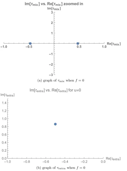
4.3 Graphs of coupling constants τmix and τextra for the A1 case when f =u= 0. (a) graph of τmix. Points are concentrated at Re[τmix] =±0.471405. (b) graph of τextra. All points are concentrated onτextra=e2πi/3, which is expected as the argument of thej-function for j= 0. 38 4.4 Graph ofτmix for theA1 case when g = 0. At this limit, all the calculated points resulted
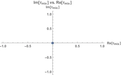
in τmix = 0. This means no mixing between the extra and visible sectors, and therefore it involves no useful information. . . 39 4.5 Graphs of components of coupling constantτmixvs. mass parameterm, whenu= 0.1 (orange)
andu= 0.01 (blue), and mass parametermtakes over values from [0,10] range. Graphs are for theA1 case. We notice that the curvature of component graphs (a and b) increase for smalleru. Graphcjust gets closer to expected Imτmix= 0, asugets closer to zero. . . 40 4.6 Graphs of coupling constants τmix1 and τextra for the A2 case when f = u = 0. (a) graph
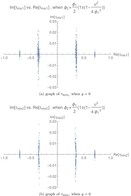
of τmix. Points are localized in bands at Re[τmix] ≈ 0,±0.35,±0.70. (b) graph of τextra. All points are concentrated on τextra =e2πi/3 =−0.5 + 0.866i, which is expected under the conditionj = 0. . . 43 4.7 Graphs of τmix1 and τmix2 forg = 0 case in A2. a. graph of τmix1. b. graph of τmix2. We
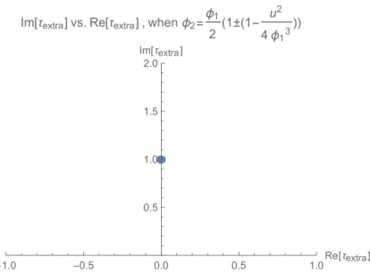
notice that, although the distribution might not be identical, but in both graphs the data points are concentrated around the same Re[τmix] values. . . 45 4.8 Graph of τextra for the g = 0 case in A2. As expected, this results in onlyτextra =i in the
fundamental domain. . . 46 4.9 Graphs ofτmix andτextra for the f = 0 case ofD4. a. In the graph of τmix the data points
are concentrated on six points, whereas inb. graph of τextra all points are concentrated on
4.10 Graphs ofτmix andτextra for theg= 0 case ofD4. a. graph ofτmix shows the values it takes whenj= 1. b. graph ofτextra, showing thatτextra=iwhenj= 1 as expected. . . 50 4.11 Graphs of the coupling constants for the weak coupling limit of D4. a. The graph ofτmix is
divided into four rectangular regions in the four quadrants. b. The graph ofτextra shows all the values ofτextraconcentrating in a band between Im[τextra]≈1.9 and Im[τextra]≈2.8. . . . 51 4.12 τmix andτextragraphs forD4symmetry group whenϕis free to take on any value in a range
equivalent to root range ofu, no constraints.a. graph of τmix. b. graph of τextra. . . 52
5.1 Graph of gaugino mixing parametersεmix(blue) and Mextra(purple) for theA1case. On x-axis we have |u|= [0,10]. In this range, εmix values are rather small, but comparable to Mextra values. . . 59 5.2 Graph of |∂Vbosonic/∂a| with respect to |u| for |u| = [0,10] for the case when there is no
superpotential. For flavor symmetry groupA1. . . 63 5.3 Contour plot of magnitude of potentialV evaluated for 15000 values ofubetween|u|= [0,1].
This graph depicts the plot of values of |V| with respect to real and imaginary parts of u. As it is evident, the magnitude of|V| barely changes, and it is definitely not at minimum at originu= 0. . . 67 5.4 Contour plots of potentialVbosonicand its derivative |∂Vbosoic/∂u|evaluated for 10000 points
LIST OF TABLES
2.1 Maximum number of supercharges for each dimension ford≤10 . . . 8
LIST OF CONVENTIONS AND ABBREVIATIONS
Our conventions follow [1]. Unless otherwise stated:
Metric signature (−,+,+,+)
Greek indicesµ, ν, . . . Lorentz indices. Run over four space-time coordinates 0,1,2,3
Greek indicesα, β, . . . spinor indices. Usually run over 1,2, forSO(3,1) Weyl spinors
Latin indicesi, j, k, l, . . . moduli space indices. Usually run over 1, .., r+1 where ris the rank of flavor symmetry group
Capital latin indicesA, B, . . . SUSY counters. Run over 1, ...,N whereN is the num-ber of supercharges
θα,θ˜α superspace coordiantes
0123 +1
SM Standard Model
SUSY Supersymmetry, Supersymmetric
SUGRA Supergravity
CHAPTER 1: Introduction
As physicists, we like to group things together neatly in a way that they can be explained by as few universal laws as possible. This is the reason why Standard Model was created throughout the latter half of the 20th century in the first place. It was formulated as a gauge quantum field theory encompassing the electromagnetic, weak, and strong nuclear interactions, as well as classifying all the subatomic particles known at the time (mid-1970’s). But although a very triumphant achievement in the history of physics, it was not so satisfying because it left out gravity and the theory of general relativity. At this point, every law known in nature belonged in only one of the two boxes of physics: that of Standard Model (or alternatively, quantum physics), and that of general relativity. And laws from one box could not even be defined in the other. In addition, the core methodologies used in these two viewpoints were intrinsically different. This inconsistency was an obstacle in the attempts to explain nature as unity. Thus began a search for a theory that can combine quantum effects with general relativity and vice versa, i.e. a theory ofquantum gravity.
But before we start discussing solutions to quantum gravity, let us talk a bit more about Standard Model (SM) and more reasons to why it is viewed as incomplete. SM was the result of impressive collaborations between both theoretical and experimental particle physicists from around the world. It was a renormalizable, mathematically self-consistent theory and it had the gauge symmetry group of SU(3)×SU(2)×U(1). SM introduced and incorporated the concept of gluons and quantum chromodynamics (QCD) to modern physics. The combining of electromagnetic and weak forces, and constructing electroweak physics, which was definitely a milestone in modern physics, was also amongst the first steps of creation of SM. The theoretical side of Standard Model also predicted the existence of several particles, which were experimentally discovered decades later1. But among all these successes, SM also had quite a few shortcomings. One of the main unsolved problems in SM is the hierarchy problem; The Standard Model leaves the mass of the Higgs boson as a parameter to be measured, rather than a value to be calculated – more of an empirical discovery, rather than a theoretical result. The only constraint on it is that it has to be of the order of 100 to 1000 GeV to ensure unitarity of SM. The problem occurs because quantum corrections require the Higgs boson to have a mass much higher than this, but for an inexplicable reason we have an almost-perfect cancellation of these corrections at∼125 GeV. The only possible explanations for this phenomenon are that there is either some underlying connections between these observations, which SM gives no explanation about, or that some
extremely precise fine-tuning must be applied on the mass parameter, which from theorists’ point of view is considered to be unnatural. Another problem with the SM are the neutrino masses; According to SM neutrinos are supposed to be massless, however neutrino oscillation experiments have shown that neutrinos actually do have mass! A third problem with SM is the inability to explain Dark Matter and Dark Energy. The SM does not have any candidates for weakly to not at all interacting Dark Matter, and the attempts to explain dark energy in terms of SM vacuum energy leads to a discrepancy of up to 120 orders of magnitude! And of course, last but not least, is the failure to couple to gravity; SM is just incompatible with gravity, or more accurately general relativity, and there is no way to incorporate gravity in the model without tearing it down with various assumptions first.
So enters the beautiful solution of String Theory. String theory, being a theory of quantum gravity, successfully answers the last shortcoming of SM listed in the previous paragraph, and also motivates various proposals to address the rest of the points. The idea is, that one can include gravity in a consistent quantum theory, if one gives up the notion that the fundamental particles in the theory must be point-like, and allow them to have one dimension, i.e. be strings [2, 3]. These fundamental strings can have a range of energies - or equivalently, masses - and thus can create different types of particles, and theories, depending on their state of oscillation. But one thing is for certain; all string theories contain a particle with zero mass and spin two [4]. In SM formulation, there exists one massless spin two particle - the graviton! Hence, all string theories will indeed contain gravity.
Consistency puts a high level of constraints on possible string theories, however. For instance, there is a family of string theories, called bosonic string theories, that are only consistent in 26 dimensions (the name comes appropriately from the fact that these type of string theories consist only of bosons!). These theories, however, also contain tachyons – which means that their ground state has a negative mass-squared value – and that makes these theories unstable. Thus, to make the theories stable and tachyon-free, we must incorporate supersymmetry - which demands that a fermion exist for each boson and vice versa2 -and this results in the theory only existing in 10 dimensions. This is therefore called supersymmetric string theory, orSuperstring theory. There are several types of superstrings, and therefore superstring theories, based on initial assumptions on whether or not allow our theory to be chiral (e.g. Type IIA superstring theory is nonchiral versus Type IIB superstring theory being chiral), or have specific gauge symmetries (e.g. Heterotic superstring theory3has anE8×E8gauge symmetry). Nevertheless, all of these different variations of superstrings have 10 dimensions.
2 This type of supersymmetry is of course broken in low-energy limits, since we do not have equal number of fermions and
bosons in nature. We will discuss an example of supersymmetcry breaking in Chapter 5.
3 Heterotic superstring theories are consistent theories that are built by combining a bosonic string theory moving in one
But as we know, the world around us in macroscopic level exists in only 4 dimensions, and in much lower energy levels than that of microscopic elements. A common approach to make contact with low energy physics, is to assume these extra dimensions are minuscule and do not appear at long distances. Mathematically, we compactify on the extra dimensions, and we get a low energy effective field theory as a result. A natural question then arises: How does string theory behave in d = 4 dimensions, i.e. the framework where Standard Model is formulated in? We know that String theory successfully couples gravity to SM, but can it provide suggestions for rest of SM shortcomings? It is undoubtedly important to examine possible low energy manifestations of String theory. In this thesis we are not going to give direct predictions of the strings, but rather we will present a well-motivated class of scenarios which canonically embed in string theory and we will use string theory to study these scenarios.
In a broad class of string-based models in F-theory, the Standard Model is given by a configuration of intersecting seven-branes [5–10]. In these configurations, the SM, also known as thevisible sector, is realized on a stack of intersecting seven-branes, 7vis. Additionally, there could also exist flavor seven-branes, 7hid. This allows for physics beyond SM to potentially enter in specific ways; many SM extensions involve the existence of so-called “extra” sectors. Probe D3-branes are very well-motivated candidates for the extra sectors, because they are locally attracted to the points of triple intersections between these seven-branes [11, 12]. The physicsbeyond SM then is studied by the “interactions” between SM (visible sector) and the extra sector (the D3-brane). In this class of models, this corresponds to the 3–7 “messenger states”; the states which are charged under both SM and the naturalU(1) of the D3-brane, U(1)D3. This encourages an investigation on mixing between theseU(1)’s. Although, generally, the electric kinetic mixing has been heavily studied [12–24], there is a substantial lack of analysis on magnetic kinetic mixing as far as we are aware [25, 26].
It is shown in [13] that the D3-brane is stable close to, but not directly on top of the 7vis brane. This realizes an N = 2 superconformal field theory (SCFT) with E8 flavor symmetry to describe the model [27, 28]. The Standard Model gauge group then comes from breaking the E8 flavor symmetry down to a GSM ≡ SU(3)×SU(2)×U(1) subgroup of the E8, which in turn has a U(1) ⊂ E8 which is commonly referred to as theU(1)-hypercharge, orU(1)Y, of the SM.
curve appearing in a special class of F-theory compactifications, commonly known as the Seiberg-Witten curve. TheSeiberg-Witten (SW) method then uses formal tools of elliptic curves to find the modular parametersτ’s of the SW curve, which in turn act as the coupling constants between the probe D3-brane and the seven-branes, i.e. between the extra and visible sectors. Indeed, Seiberg and Witten used this method to write an exact low-energy effective Lagrangian for N = 2 supersymmetric theory withSU(2) gauge theory [37]. This was later generalized toSU(N) gauge groups in [38, 39], and then even more generalized for the cases with exceptional Lie groups as gauge groups, or even cases where the gauge group is not specified and we cannot propose a Lagrangian [27, 40].
The fine point of the SW method is that the N = 2 supersymmetric gauge theory contains a complex adjoint matrix scalar, whose non-zero vacuum expectation value parameterizes physically distinct vacua. Thus, we can always write its effective field theory as a bundle of U(1)’s [41]. This is because in four-dimensionalN = 2 theories, the definitive K¨ahler potential of the theory is also constrained by holomorphy [42], hence we can make exact statements for four-dimensional strongly coupled field theories without knowing much about the details of the theory. This ability is what makes the four dimensional string theories, and specifically thed= 4,N = 2 supersymmetric theory, much interesting subjects in field theory.
In our work, instead of E8 flavor symmetry which has all of the SM gauge group as a subgroup, we assume different, smaller gauge groups with various flavor symmetries, with the presumption that the flavor symmetry of these groups would at least partially encompass the SM gauge group. Using the SW method then, with proper choice of parameters we can extract aU(1) from these flavor symmetry groups; then the interaction between the visible and extra sectors is summarized in the interaction betweenU(1)D3 and the extracted U(1)’s from the flavor symmetry group. For these flavor symmetry groups, we find the modular parameters of the SW curve, which in turn are thecoupling constantsτij’s between the probe D3-brane and the seven-branes, i.e. between the extra and visible sectors. These calculations form the heart of this thesis.
is hardly interacting with the visible sector means this extra sector provides natural candidates for Dark Matter. The extra sector with these configurations is often referred to as the “Dark sector”. The electric kinetic mixing, from concepts similar to that of Dark sector, has been studied widely and resulted in several DM scenarios [22, 43–47]. However, in our scenario, we treat the physics of the Dark sector as one with
N = 2 supersymmetry, as well as both electric and magnetic kinetic mixing. This gives rise to very interesting possibilities for DM phenomenology that could be probed in DM experiments. For example, a recent review on composite dark matter scenarios with strong coupling dynamics can be found in [48].
The structure of this dissertation is as follows: in the next chapter I introduce supersymmetry and lay down the mathematical groundwork for four dimensional supersymmetric theories. In the following chapter I present details for our model and talk about the mixing terms between visible and extra sectors at both weak and strong coupling limits; the need to work in strong coupling then shapes the main motivation of this project. This brings the culmination to Chapter 4 where I introduce the Seiberg-Witten method and carry coupling constant calculations for various flavor symmetry groups, namely A1, A2 andD4. Chapter 5 is dedicated to the effects of supersymmetry on the field theory; specifically, I calculate the bosonic and fermionic masses of the theory once in the supersymmetric limit, then I introduce supersymmetry breaking and see how the mass values diverge from each other when there is no supersymmetry. Eventually, in Chapter 6 I explore the concept of the dark sector; more specifically, I investigate Dark Rutherford scattering by treating a magnetically charged extra sector as a heavy classical source, and scatter charges (in case of direct detection experiments, most probably protons) off this source. The charges represent the visible sector and the model itself assimilates Dark Matter moving around the earth in galactic wind. We finish the dissertation with providing summary of results and an outlook of future prospective work in Chapter 7.
CHAPTER 2: A Look Into Supersymmetry
Supersymmetry is one of the most compelling fields of study in modern physics, because it suggests solutions to several problems that are otherwise prominent in Standard Model. For instance, it has a natural solution to the hierarchy problem between the electroweak scale and the Planck scale. Supersymmetry (or SUSY, for short) also leads to gauge coupling unification at high energy (GUT scale) where Standard Model fails to do so. In addition, extensions of supersymmetry also provide Dark Matter candidates which are consistent with relic abundance calculations; we will explore a toy model of such candidates in Chapter 6. Because of these reasons and several more, supersymmetry has become the dominant framework in string theory.
In this chapter we will lay down the mathematical groundwork for formulating supersymmetry. This will begin by presenting the SUSY algebra. For the most part, we will focus on SUSY in 4 dimensions because this will be the most prominent case throughout this dissertation. However, generalizations to other dimensions will be discussed briefly.
Section 2.1: SUSY algebra
In its simplest form, SUSY inddimensions can be described by generatorQαand its conjugate ¯Qα˙. By Lorentz invariance these generators are spinor representations ofSO(d−1,1). In d= 4 therefore, they are SO(3,1) Weyl spinors and they abide the following anti-commutation relations,
{Qα, Qβ}={Q¯α,˙ Q¯β˙}= 0
{Qα,Q¯β˙}= 2σαµβ˙Pµ (2.1)
where Pµ is the energy-momentum operator (the four-momentum in d = 4) and the index µ,(ν, ...) runs from one to four identifying Lorentz four-vectors. The indicesα, β, ...,α,˙ β, ...˙ run from one to two to denote the two-component Weyl spinors. Alsoσµ = (1, σi), whereσi, i= 1,2,3 are the three Pauli matrices. It is also worthwhile to introduce the ¯σµ notation,
σµ
αβ˙ = (1, σ i
There is one more additional relation for SUSY algebra, and that comes from the fact that this symmetry does not depend on spacetime position; therefore
[Qα, Pµ] = [ ¯Qα˙, Pµ] = 0. (2.2)
We also have the trivial [Pµ, Pν] = 0.
The generator Qα is called thesupercharge of the theory, since it exchanges superpartner states with each other. In other words, because Qα is a spinor, it turns bosons into fermions and vice versa according to the spin-statistics theorem. This is commonly written in a formal notation as
{(−1)F, Qα}= 0
where
(−1)F|bosoni= +1|bosoni (−1)F|fermioni=−1|fermioni. (2.3)
The relations (2.1) and (2.2) describe the formulation of the simplest form of supersymmetry, with only one supercharge Qα. Generally we can have multiple supercharges governing the supersymmetry of the theory. In these cases we adopt an additional index for the supercharges and write them as QA
α, where A= 1, ...,N for a theory with N supercharges. Theories withN >1 SUSY are then referred to as having
extended SUSY; in return, theN = 1 SUSY described above adopts the nameunextended supersymmetry. The extended SUSY algebra in 4 dimensions then follows the following relations,
{QAα,Q¯βB˙ }= 2σµ αβ˙Pµδ
A B
{QAα, QBβ}= 2αβZAB
{Q¯αA,˙ Q¯βB˙ }=−2α˙β˙Z AB†
[QAα, Pµ] =[ ¯QαA, Pµ] = 0˙ (2.4)
with [Pµ, Pν] = 0 and α˙β˙ =−αβ. As already mentioned, A, B, ... = 1, ...,N; the rest of the indices run similar to the unextended case as described under (2.1). TheZABhere are antisymmetric linear combinations of internal symmetry generatorsTi,
ZAB= X
i ciABT
i
d N
10 2
9 2
8 2
7 2
6 4
5 4
4 8
3 16
Table 2.1: Maximum number of supercharges for each dimension ford≤10
and they commute with all other operators in the algebra. Because of this, the ZAB are called the central
charges of the algebra.
There is a maximum number of supercharges a theory can have in each dimension, however. This number is decided by the constraint that no particle with spin larger than 2 should exist in the theory [49]. For d= 4 this number isN = 8; this is equivalent to 32 degrees of freedom. Indeed, each Weyl spinor has four degrees of freedom (Q1, Q2,Q˙¯1, and ¯Q˙2) and 8×4 = 32. This is referred to as maximal supersymmetry. The maximal supersymmetry is closely associated with gravity; in some dimensions being the only case that includes the spin 2 particle graviton in its representations. Supersymmetric theories which include graviton (and its superpartnergravitino) are calledsupergravity theories, or SUGRA.
The maximum number of supercharges in dimensions other than four should also result in 32 maximum degrees of freedom for the theory. A list of maximum allowed number of supercharges in each dimension (d≤10) is shown in Table 2.1, borrowed partially from [50].
Section 2.2: SUSY Multiplets and Representations
2.2.1: Massless multiplets
We will now explain how to achieve the states in each supersymmetric theory using its SUSY generators QA
α. For this we will start with the more straightforward case of massless multiplets first.
Since massless states do not have a rest frame, they are best described in the light frame;Pµ= (E,0,0, E) whereE is the energy of the state. A massless state is determined by its energy and its helicityλ. Combined it can be represented as|E, λi.
We now introduce an auxiliary operator called thePauli-Lubanski pseudo-vector,
Wµ=−1
2
HereMµν is Lorentz rotation generator and it commutes with the SUSY generators like,
[QAα, Mµν] = 1 2(σµν)
β αQ
A
β [ ¯Q A
˙
α, Mµν] =− 1 2(¯σµν)
˙ β ˙ αQ¯
A ˙ β.
The zeroth component of the pseudo-vector (2.5) has a convenient eigenvalue when acting on a massless state,
W0|E, λi=Eλ|E, λi
the product of the energy and helicity of the state! Therefore we will now try acting withW0 on the state QA
α|E, λi. We will have
W0QAα|E, λi=QAαW0+ [W0, QαA]|E, λi=Eλδβα−1
2(σ 3)β
α
QAβ|E, λi (2.6)
But we know that (σ3)1
1 =−(σ3)22 = 1 and (σ3)21 = (σ3)12 = 0. Therefore this means thatQA1 lowers the helicity by1/2andQA
2 raises it by1/2.
Alternatively, if we write (2.6) for the conjugate generators we will see that ¯QA ˙
1 would raise the helicity by1/2and ¯QA
˙
2 would lower it by
1/2. Therefore we can setQA
2 = ¯QA2˙ = 0 and define “creation/annihilation” operators only usingQA
1,Q¯A1˙ . Assume
aA≡ 1
2√EQ A
1 a
A†≡ 1 2√E
¯ QA1˙.
These operators will then abide a simple Clifford algebra,
{aA, aB†}=δAB {aA, aB}={aA†, aB†}= 0.
Now that we have creation and annihilation operators we can start constructing our states starting by the ground state. By definition, a ground state|E, λ0iwould vanish by all annihilation operators. In other words,
aA|E, λ0i= 0 ∀A= 1, ...,N
The rest of the states would then just be created by acting on the ground state by one or multiple creation operators. Each creation operator would raise the helicity by1/2.
The maximum number of creation operators acting on the ground state is of course capped byN. Also, for each state|E, λ0+k
0
/2i, there would be Nk0
ways of achieving it. These two statements are what we use to construct our multiplets!
I will bring examples of constructing several multiplets that are pivotal to the work in this dissertation in the following.
N
= 1
Multiplets
When N = 1, that means that k in (2.7) has only one value, which in turn means only one creation operator.
Chiral Multiplet
This multiplet has the ground state helicity of λ0= 0. Therefore the states will be
|E,0i
a†|E,0i=|E,1 2i
The physical content of this multiplet is one complex scalar field and one Weyl spinor. Vector Multiplet
This multiplet starts with ground state helicity ofλ0=12. The states are
|E,12i
a†|E,12i=|E,1i
The field content of this multiplet is a two-component spinor again (gaugino) and a vector boson (gauge boson).
These are the mainN = 1 multiplets we will encounter going forward.
N
= 2
Multiplets
This multiplet starts with helicityλ0= 0 again. The states will be
|E,0i
a†1|E,0i=|E,12i
a†2|E,0i=|E,12i
a†1a†2|E,0i=|E,1i
The field content of this multiplet is a vector boson, two spin 1/2 fermions, and a complex scalar field.
The Hypermultiplet
Ground state of this multiplet has helicityλ0=−1
2. Therefore,
|E,−1
2i
a†1|E,−1
2i=|E,0i
a†2|E,−1
2i=|E,0i
a†1a†2|E,−1
2i=|E,
1
2i
The field content would be a Weyl fermion ψ, two complex scalarsqand ˜q, and another Weyl fermion ˜
ψ in the conjugate representation ofψ.
The N = 2 multiplets can be decomposed in terms of N = 1 multiplets. In the language of N = 1 multiplet, the N = 2 vector multiplet can be considered as the N = 1 vector multiplet plus the chiral multiplet. TheN = 2 hypermultiplet can be thought of as the N = 1 chiral multiplet plus its conjugate.
N
>
2
Multiplets for Additional Examples
N = 4 Vector Multiplet
states and multiplicities then are:
4 0
= 1 |E,−1i
4 1
= 4 a†1|E,−1i=|E,−1
2i
4 2
= 6 a†1a†2|E,−1i=|E,0i
4 3
= 4 a†1a†2a†3|E,−1i=|E,12i
4 4
= 1 a†1a†2a†3a†4|E,−1i=|E,+1i
N = 8 SUGRA Multiplet
This is the maximal SUSY in d= 4 and it will have a spin 2 graviton. The states start with ground state helicity ofλ0=−2. Then
8 0
= 1 |E,−2i
8 8
= 1 (a†)8|E,−2i=|E,+2i
8 1
= 8 (a†)1|E,−2i=|E,−3/2i
8 7
= 8 (a†)7|E,−2i=|E,+3/2i 8
2
= 28 (a†)2|E,−2i=|E,−1i
8 6
= 28 (a†)6|E,−2i=|E,+1i
8 3
= 56 (a†)3|E,−2i=|E,−1/2i
8 5
= 56 (a†)5|E,−2i=|E,+1/2i 8
4
= 70 (a†)4|E,−2i=|E,0i
All of the discussion brought in this section was about massless states and multiplets. Next we will study the massive multiplets.
2.2.2: Massive BPS multiplets
Let us refer back to the fact that in the massless multiplets, the number of states with each helicity was defined by Nk
. This means that the total number of states in a massless multiplet is
N X k=0 N k
= (1 + 1)N = 2N.
like the SUSY generatorsQAα. Thus the total number of states in a massive multiplet would be 2N
X
k=0 2N
k
= 22N.
This is problematic for various reasons. Firstly, assuming fields become massive under Higgs mechanism, we cannot go from a multiplet with 2N states to one with 22N states; quantum corrections cannot change the length of the multiplet. Furthermore, and we will get to talk about this concept more in the next chapter, while studying the strong coupling limit of supersymmetric theories, 22N includes too many degrees of freedom and result in inconsistent mass values. By contrast, multiplets with 2N degrees of freedom have mass/charge ratios that are fixed by SUSY algebra and are preserved under a continuous variation in the gauge coupling.
To fix this issue let us return to (2.4). As mentioned, the central charges ZAB are anti-symmetric, and since they commute with everything they can be diagonalized. For this purpose we choose to work in a basis where the matrixZAB can be written as
ZAB =
0 D
−D 0
where theD-block is anN/2×N/2diagonal matrix with eigenvalueszm on the diagonal,m= 1, ...,N/2.
D= diag(z1, ..., zN/2)
We will now divide the indices A = 1, ...,N into sets of double indices (A, m) where A = 1,2 and m= 1, ...,N/2. Therefore the extended SUSY algebra would then read
{Q(A,m)α ,Q¯(B,n)˙ β }= 2δ
ABδmnσµ
αβ˙Pµ (2.8)
{Q(A,m)α , Q(B,n)β }= 2αβABδmnzm
{Q¯(A,m)α˙ ,Q¯(B,n)˙
β }=−2α˙β˙ ABδmn
zm
It is also worthwhile to mention that for massive states we can always operate in their rest frame, where Pµ= (M,0,0,0). Therefore the first line of (2.8) becomes
{Q(A,m)α ,Q¯(B,n)˙
sinceσ0=1.
We can make the sets of relations in (2.8) more compact by defining new generators,
Q± αm≡
1 2 Q
(1,m) α ±Q¯
˙
α(2,m), (2.9)
and their Hermitian conjugates Q±αm, where plus and minus act respectively. The dotted and undotted indices in (2.9) are mixed while preserving covariance; another way of writing this would be to replace ¯Qα˙ withαβ˙Q¯β˙.
The SUSY algebra (2.8) with these new operators will then be
{Q± αm,Q
± βn}={Q
± αm,Q
∓ βn}={Q
± αm,Q
∓ βn}= 0
and
{Q±αm,Q±βn}=δαβδmn(M ±zm). (2.10)
But the left hand side of (2.10) is non-negative, so that requires
M ≥zm (2.11)
In other words, the mass of the state is bounded from bottom by the eigenvalues of central charges. The condition in (2.11) is known as theBPS bound, and states abiding by this bound as BPS states.
Suppose condition (2.11) is satisfied for N eigenvalues zm. Then we can rescale the operators Q±αm for thoseN eigenvalues by defining
a±αm ≡(M ±zm)− 1 2Q±
αm
The operators a±αm are creation/annihilation operators whose degrees of freedom is reduced by N bound states. Therefore they follow a Clifford algebra with 2(N −N) degrees of freedom. This means that the total number of states becomes
2N X
k=0
2(N −N) k
= 22(N −N).
It is easy to see here that the maximum number of zm eigenvalues which can satisfy the BPS bound is
Section 2.3: Supersymmetric Field Formulation
Let us remember once again the field content ofN = 1 SUSY multiplets:
chiral multiplet- consists of a complex scalar fieldφand a two-component spinorψα
vector multiplet - consists of a massless vector field Aµ (gauge boson) and its superpartner λα (gaugino)
Hereα= 1,2 andµ= 0,1,2,3 as usual.
In SUSY theories, for further calculation purposes, and to be able to write SUSY invariant Lagrangians, it is convenient to combine the consisting fields of these multiplets into so-called superfields. So let us investigate each of the aforementioned multiplets from QFT point of view.
For the chiral multiplet, we will introduce anticommuting variables θα and ¯θα, and an auxiliary field˙ F to assembleφandψinto the chiral superfield Φ.
Φ =φ(y) +√2θψ(y) +θ2F(y) (2.12)
whereyµ =xµ+iθσµθ. One should realize that by¯ θ2 we mean θθ=θαθ
α, the same way byθψ andθσµθ¯ we mean the summationsθαψα andθασµ
αα˙θ¯α˙, respectively. Expanding they-dependance would give us
Φ =φ(x) +iθσµθ∂µφ(x)¯ −1
4θ
2θ¯2∂2φ(x) +√2θψ(x)−√i 2θ
2(∂µψ(x)σµθ¯+θ2F(x) (2.13)
Here we utilized the fact thatθ’s are anticommuting andθαθα= 0.
For the vector multiplet we will again use the θ’s and another auxiliary field D to assemble the vector superfield V.
V =−θσµθAµ¯ +iθ2(¯θλ)¯ −iθ¯2(θλ) +12θ2θ¯2D (2.14)
The fields in the vector multiplet can be put together in a different way to create a more complex superfield which would prove to be very useful in further calculations. This superfield is
Wα=−iλα(y) +D(y)θα−iσµναβθβFµν+θ2σµ∇µλα(y)¯ (2.15)
Here σµν = 1
4(σ
So now, since Wα is chiral, the contraction WαWα would be SUSY invariant. One then is curious to calculateR
d2θWαW
α, knowing that R
dθ≡ ∂
∂θ. This means that the result of the integral would simply be the coefficient of theθ2term of theWαW
αexpansion. So,
WαWα θ2 =
h
−iλα(y) +D(y)θα−iσµν,αβθβFµν+θ2σ∇λ¯α(y) i
×h−iλα(y) +D(y)θα−iσικαβθ β
Fικ+θ2σ∇¯λα(y)i θ2 = −2iλσµ∇µλ¯+D2−i(σµν)ααDFµν−
1 2σ
µνσικFµνFικ θ2
But (σµν)αα= Trσµν = 0. Also,
σµνσικ= 1 2(g
µι
gνκ−gµκgνι)− i
2 µνικ
(with0123= +1). So eventually, we will get to the SUSY invariant result,
Z
d2θWαWα=−1
2FµνF
µν−2iλσµ∇
µλ¯+D2+ i 2Fµν
˜ Fµν,
where we have replaced the dual ˜Fµν ≡ 1
2
µνικFικ in the last term.
This expression appears to have potential to be a Lagrangian, but it needs some changes. Most impor-tantly, it’s last term is purely imaginary, which cannot happen in an invariant Lagrangian. However, if we introduce the complex coupling constant
τ= θ 2π+
4πi
g2 , (2.16)
and calculateR
d2θτ WαW
αinstead, then we could get a real Lagrangian with correct coefficients. Indeed, 1
8π Im Z
d2θτ WαWα= 1 8π ·
h4π g2(−
1 2FµνF
µν−2iλσµ∇
µ¯λ+D2) + θ 2π
1 2Fµν
˜ Fµνi
= 1 g2· −
1 4FµνF
µν−iλσµ∇ µλ¯+
1 2D
2+ θ
32π2FµνF˜
µν. (2.17)
CHAPTER 3: Stringy Extensions To Standard Model
Before we begin any discussion about physics beyond Standard Model, we first need to describe the Standard Model in the platform of string theory. In a broad class of string-based models, the Standard Model is given by a configuration of intersecting seven-branes via F-theory (see for example [5, 6], or for more extensive literature on model building in F-theory [7–10]). From this point of view then, many SM extensions involve the existence of so-called“extra” sectors. Let us describe an example of such configurations.
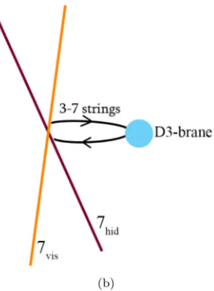
In these configurations, the SM is localized at the intersection of a stack of seven-branes 7vis; this is also known as thevisible sector. Additionally, there could also exist extra flavor seven-branes 7hid. At the points of triple intersections between these seven-branes, Yukawa interactions are localized. This motivates another good choice for extra sector. Probe D3-branes are locally attracted to Yukawa points [11, 12], so we can include their “interactions” with the seven-branes. It is important for visualization to note that these branes are spacetime filling branes, with seven-branes filling four extra dimensions, while D3-branes are pointlike in extra dimensions. For a visual depiction of this scenario, see Figure 3.1.
Our goal is of course to study physics beyond the Standard Model; therefore we will focus on the “in-teractions” between SM (visible sector) and the extra sector, which is the D3-brane. The two communicate with each other via “messenger states”, which in the case of this model correspond to the 3–7visand 3–7hid strings (see Figure 3.1b). The D3-brane has a naturalU(1) gauge group which we will denote byU(1)D3. The 3–7vis states are charged under both SM and U(1)D3, while the 3–7hid ones are only charged under U(1)D3 and are SM singlets, and therefore are much lighter. Because of these properties, the 3–7hidstates form a natural candidate for Dark Matter, i.e. adark sector; we will revisit this concept in Chapter 6. But until then, we will explore more generally the physics of all states charged underU(1)D3; which means the 3–3, 3–7vis and 3–7hid string states.
It is worth reiterating again, that the 7–7 intersections realize the Standard Model. More specifically, the 7vis–7vis string states are associated with force carriers of SM, while 7vis–7hid states represent the quarks and leptons. The 7hid–7hid intersection of the flavor branes is a weakly coupled extra sector, that can also be viewed as a possible scenario for Dark Matter. This possibility was studied in [51].
(a) (b)
Figure 3.1: Depiction of interaction between the Standard Model and the extra sector. a. Shows the general scheme and the “messenger” states. Under “Visible sector” can be any flavor symmetry group that partially includes SM gauge groupGSM. The “Extra sector” is the probe D3-brane. b. Pictures the model described in this chapter. The 7vis seven-brane stack gives the SM gauge group (or replacements), and the 7hid stack corresponds to a flavor seven-brane. Their intersection creates the Yukawa points, and close to Yukawa point is the probe D3-brane as extra sector. The two sectors interact with each other via 3–7 messenger string states.
“Minahan-Nemeschansky theory” [27, 28]. The Standard Model gauge group then comes from weakly gauging aGSM≡SU(3)×SU(2)×U(1) subgroup ofE8.
Instead ofE8, which has all ofSU(3)×SU(2)×U(1) as a subgroup, in this project we will start small! We will assume different gauge groups for our visible sector with various flavor symmetries, with the presumption that the flavor symmetry of the group would at least partially encompass the SM gauge group. With proper choice of parameters then, we can extract a U(1) from the flavor symmetry groups too. The interaction between the visible and extra sector then, would be summarized in the interaction between theU(1)D3 and the extractedU(1) from the flavor symmetry group.
In the next chapter, we will investigate several different flavor symmetry groups and explore the model in each case. In this chapter, however, we will set up the framework that will be needed for these calculations.
Section 3.1: Weak Coupling Limit
would be
L=−1
4 n 1
g2 11
Fµν1 F1,µν+ 1 g2 22
Fµν2 F2,µν+ 2 g2 12
Fµν1 F2,µνo
+ 1
32π2 n
θ11Fµν1 F˜ 1,µν
+θ22Fµν2 F˜ 2,µν
+ 2θ12Fµν1 F˜
2,µνo
, (3.1)
whereFi
µνs are field strengths ofU(1)i, and their duals are defined as ˜Fi,µν = 1 2
µνρσFi
ρσ. The Lagrangian (3.1) can be rearranged to be written as
L=− 1
4g2 11
Fµν1 F1,µν− 1 4g2
22
Fµν2 F2,µν+ θ11 32π2F
1
µνF˜1,µν+ θ22 32π2F
2
µνF˜2,µν+Lmix,
where
Lmix=− χelec
12 2 F
1 µνF
2,µν−χ
mag 12
2 F 1 µνF˜
2,µν.
The terms with duplicate indices are simply the well-known formulation for singleU(1) scenarios. The
mixing effect between the twoU(1)’s is represented in the terms proportional toχelec
12 andχ
mag
12 . The χelec12 term is the CP preservingelectric mixing term between the twoU(1)s
Fµν1 F2,µν=E~1·E~2−B~1·B~2,
while the term proportional toχmag12 , is CP violating and can be written as
Fµν1 F˜ 2,µν
=E~1·B~2+B~1·E~2,
and represents the mixing of the magnetic and electric fields of differentU(1)’s with one another; this will be themagnetic mixing term.
Just like any other situation in quantum field theory, we first assume that these coupling constants are small and proceed to solve our problem using weak coupling methods. The most common tool at weak coupling is perturbation theory with Feynman diagrams. So let us figure out the Feynman diagrams associated with the Lagrangian (3.1).
Feynman diagram associated with these transition would be
Figure 3.2: Feynman diagram showing the transition between γ1 andγ2 of two differentU(1)s.
At second order in the case of twoU(1)s, we would have the vacuum polarization diagram transitioning γ1to γ2 through a loop of creation and annihilation.
Figure 3.3: vacuum polarization diagram of two different U(1)s showing transition betweenγ1 andγ2.
The modified Green’s function for this diagram would be
−
Z d4k (2π)4Tr
h
−ig1γµ· i /
p−m· −ig2γ ν· i
/ p0−m
i
, (3.2)
where g1 and g2 are charges of the fermions, i.e. g1 =e1q1, g2 = e2q2, with theei being the unit charges under eachU(1)i. pandp0 are the momenta of the fermion and anti-fermion created, andmis their mass.
A review of a similar Green’s function calculation has been presented in [52]. The final result for a 4-dimensional spacetime with slight modification would match ours,
−2χ
π Z 1
0
dxx(1−x)2
−γ−log∆ + log 4π
.
Here, instead of the familiarα= e 2
4π, we have introduced the modifiedχ≡
q1e1q2e2 4π .
In addition, ∆≡m2−x(1−x)k2, withkbeing the momentum of the photons. Sincexonly ranges from 0 to 1, for large mass values, ∆≈m2and thus log∆≈2logm. This will get rid of all the constant terms in the parenthesis1, and as a result we will be left with
2χ
π ·2logm· Z 1
0
dxx(1−x)
=q1e1q2e2 6π2 log
m
µ, (3.3)
1 The terms 2
−γcome from a Gamma function approximation and always cancel in observable quantities. The scheme used
whereµis a reference scale.
Now consider a toy model with four fermionsf1, f2, f12, f120 with respective charges (q1,0),(0, q2),(q1, q2), (q1,−q2) underU(1)1×U(1)2 gauge symmetry. And also respective masses ofm1, m2, m12, m012. According to (3.3), the fermionsf1andf2will not have a contribution to the Green’s function since the product of the charges would vanish. Forf12andf120 on the other hand, we will have the combined contribution of
q1e1q2e2 6π2 log
m12 m0
12
. (3.4)
This result presents two very important ideas. One, that for there to be a mixing effect, matter needs to be charged under bothU(1)s. Two, it gives rise to “non-decoupling effect”; meaning that even if the masses are too large to have an effect in the weak coupling limit, if they’re comparable (and charged oppositely under one of theU(1)s), the effect would still be present.
The expression written in (3.4) is thecoupling constant for the weak coupling limit. This result was first presented by Holdom in [21].
At this point one should note that unless there are magnetic monopoles in the theory, the θ terms and the entirety of second line in (3.1), can be ignored because being a total derivative, they do not add any new information to the equations of motion. Therefore, in order to see effects of magnetic mixing, and to proceed with our calculations, it is necessary to assume that magnetic monopoles exist.
More so, it is important to remember that weak coupling, and therefore the method of Feynman diagrams, is a perturbative one. Indeed, in the weak coupling limit we assume that the monopoles are heavy. More specifically,
mmonopole melectron ∝
1 g2
whereg <<1. It is then of natural curiosity (and a well-motivated one, as it will become clear later in this thesis), to explore the limits where the mass of electron and mass of monopole are comparable; i.e. when g≈1. In these limits, we cannot claim perturbation anymore, and thus we exit the weak coupling territory.
Section 3.2: Strong Coupling Limit
Let us have a quick review of Maxwell equations in presence of monopoles. The original Maxwell equations (without the monopoles) are summarized as
∂µFµν =Jeν
whereFµν is the electromagnetic field tensor, defined asFµν =∂µAν−∂νAµ, andJeνis the electric current. The presence of monopoles, as we know, encourages aduality in the equations (3.5). They become
∂µFµν=Jeν
∂µF˜µν=Jmν, (3.6)
where Jν
m is the magnetic current, which is defined analogous to the electric current. However, with the monopoles involved, the field tensor is no longer the antisymmetric difference of derivatives of the vector potential.
Unlike electric mixing, magnetic mixing does cause CP violation in the theory. Indeed, according to Dirac [53], if we have a particle with electric charge q and another particle with magnetic charge p, the quantum mechanics of their interactions would only be consistent if pq = 2πn. Additionally, it was shown in [54, 55] that a generalized version of this condition also holds for dyons. Namely, if we have a dyond1, with electric chargeq1and magnetic chargep1 (we will incorporate the shorthand notationd1= (q1, p1) for dyons), and another dyon d2= (q2, p2), the quantum mechanics between them would only be consistent if q1p2−p1q2= 2πn. This quantity is often calleddyon coupling between the two dyons,
hd1|d2i ≡q1p2−p1q2.
It is of interest to note, that one can now treat a separated dyon as two distant special dyons, where one only has electric charge and the other only magnetic. In other words, one would haved1= (q,0) andd2= (0, p). In this special case then, the dyon coupling is also going to be the system’s angular momentum, as we will havehd1|d2i=pq≡ |~l|. The derivation of this equation is shown in length in Chapter 6, but it is worthy to notice here that the quantization of the angular momentum of the system is equivalent to the quantization of electric and magnetic charges.
Now let us imagine a dyon with electric charge q and minimum magnetic charge p = 2πe, i.e. (q,2πe). When we act on this dyon with the CP operator, since electric and magnetic fields transform oppositely under parity, then the resulting dyon would have (−q,2πe). Comparing these two particles then, we would have q1p2−p1q2= 4πqe . This is only a multiple of 2πifq=neor q= (n+1
2)e. Therefore, dyons must all have either integer or half-integer electric charges.
work in a basis in which all magnetic charges are integral and in which the physically measured electric charges may contain shifts by various theta angles [56].
Let us first note that we can write the general θ-terms as
− θ
32π2FµνF˜
µν = θ
8π2E·B. (3.7)
In a background with magnetic monopoles theEandBfields would be defined using the electromagnetic potentialAµ= (A0,A) as followed,
E=∇A0 B=∇ ×A+pr
r3,
wherepis the magnetic charge of a monopole located at the origin. Now if we calculate the θ-term contri-bution to the Lagrangian (using (3.7)), we will get
Lθ= θ 8π2
Z
d3rE·B= θ 8π2
Z
d3r(∇A0)·(∇ ×A+pr r3) =− θp
8π2 Z
d3rA0∇ · r
r3 =− θp 2π
Z
d3rA0δ3(r).
This is similar to the interaction of an electric point charge with the magnitude of θp2π located at the origin, i.e. where the monopole is, with the electrostatic potentialA0. Considering the agreed upon basis wherep is integer, then we can say that the dyon has acquired a shift in its electric charge by integer× θ
2π.
This calculation can be used for θ11 and θ22; in each case it would give us the electric charge of that monopole under its correspondent U(1). The θ12 term however, would give us the “mixing” charges. To calculate this for example we will write the electric and magnetic fields of both U(1)s in presence of a monopole that has magnetic chargep2 underU(1)2. In other words,
E1=∇A01, B1=∇ ×A1, E2=∇A02, B2=∇ ×A2+p2
r
r3.
We will then have
Lθ= θ12 8π2
Z
d3r(E1·B2+E2·B1) =− θ12 8π2
Z
d3rA0∇ ·pr r3 =−θ12p2
2π Z
d3rA01δ3(r).
This indicates that this dyon has now acquired an electric charge shift by θ12p2
acquired a shift in its electric charge affected by the monopole of the extra sector, which is charged under U(1)2.
As we mentioned earlier in our discussion, with including monopoles we are enhancing a duality between electric and magnetic fields. This suggests that electric mixing and magnetic mixing, could be two faces of the same coin! In fact, we could nicely package the two together with the help of a complex matrix τij defined as
τij= θij 2π +
4πi g2
ij
. (3.8)
This is the most central expression of this thesis. From here on, whenever we mention “coupling constants” or “coupling constant matrix”, we will be referring to the matrixτij and its elements.
Now, utilizing the coupling constant matrixτij, we can write the Lagrangian (3.1) as
L= 1 16π
−ImτijFµνi Fj,µν+ ReτijFµνi F˜j,µν
(3.9)
It is easy to check that this will give us the same Lagrangian as (3.1). Indeed,
L=− 1
16πImτijF i µνF
j,µν+ 1
16πReτijF i µνF˜
j,µν
=− 1
16π 4π g2
ij
Fµνi Fj,µν+ 1 16π
θij 2πF
i µνF˜
j,µν
=− 1
4g2 ij
Fµνi Fj,µν+ θij 32π2F
i µνF˜
j,µν.
As one can notice, the real part of (3.8) gives the magnetic mixing terms (Reτij is proportional to the magnetic coupling constants θ), while the imaginary part of the statement gives the electric mixing terms (Imτij is proportional to the electric coupling constants g12). So it becomes evident that knowing theτij will give us all we need to know about the mixing terms with the extra sector.
In the next chapter, we will introduce a method that will help us find theτij’s. But before that, we will need to introduce the necessary fields and framework in which this method operates and that is theN = 2 supersymmetric quantum field theory. The next section is dedicated to superfield formulation of N = 2 SUSY.
Section 3.3: N = 2 Superfield Formulation
the vector multiplet, into a singleN = 2 supersymmetric multiplet. Conceivably, this multiplet would have two sets of fermions (spinorsψand gauginoλ) and two sets of bosons (the complex scalarφand the gauge bosonAµ). A SUSY invariant Lagrangian for this multiplet then, would also come from combining SUSY invariant expressions consisting of theN = 1 superfields.
We have already found one such combination using the spinorial superfields, (2.17). Another SUSY invariant expression can be constructed by combining the chiral and vector superfields as follows
Z
d2θd2θΦ¯ +e−2gVΦ.
These two expressions put together, with some coefficient adjustment, would create the N = 2 super Yang-Mills Lagrangian
L= 1 8π Im
Z
d2θτ WαWα+ 1 2g2
Z
d2θd2θΦ¯ +e−2gVΦ = Imh τ
8π Z
d2θWαWα+ Z
d2θd2θΦ¯ +e−2gVΦi.
It can be shown that the two integrals above can be combined into one single equation,
L= Imh τ 8π
Z
d2θd2θ˜1 2Tr Ψ
2i, (3.10)
where Ψ is theN = 2 analogue of a chiral superfield, and ˜θα,θ¯˜α˙ are a new set of anticommuting variables introduced forN = 2 SUSY. The explicit form for Ψ can therefore be obtained as
Ψ = Φ(˜y, θ) +√2˜θαWα(˜y, θ) + ˜θαθαG(˜˜ y, θ), (3.11)
with
G(˜y, θ) =−1
2 Z
d2θ[Φ(˜¯ y−iθσθ, θ,¯ θ)]¯ +exp{−2gV(˜y−iθσθ, θ,¯ θ)¯}
and ˜yµ = xµ+iθσµθ¯+iθσ˜ µθ¯˜=yµ+iθσ˜ µθ. The superfields Φ(y, θ),˜¯ Φ(x, θ,θ), V¯ (x, θ,θ) and¯ W(y, θ) are given by their N = 1 description, respectively (2.12),(2.13),(2.14) and (2.15). All the component fields are in the adjoint representation ofSU(N) gauge symmetry.
One could notice from (3.10) that the integrand depends only on Ψ, and not Ψ+. Indeed, the most all-inclusive form of writing theN = 2 SUSY Lagrangian is
LN=2= 1 8πIm
Z
where the function F is aholomorphic function of Ψ, meaning that it is only a function of Ψ and not Ψ+. This functionFis called theN = 2prepotentialand it is a very important object inN = 2 supersymmetry. In particular, if we define it asF(Ψ)≡1
2TrτΨ
2, we will return to the Lagrangian (3.10).
Furthermore, if we expand Ψ according to (3.11), and consequently (2.12), we will notice that its bosonic component involves the adjoint valued complex scalar fieldφ. Let us now assume a ground state in which the adjoint fieldφhas a non-zero vacuum expectation value. At weak coupling limit, this can be parameterized in terms of a diagonalN×N matrix, whereN =r+ 1 andris rank of the gauge group. We have,
φ=
a1 . ..
aN
, (3.13)
witha1+...+aN = 0. The situation is slightly different in strong coupling limit, because there we should parameterize the vacuum only in terms of vacuum expectation values of gauge invariant operators. By multiplying this matrix by itself and taking the trace of the product diagonal matrices, we can create N−1 =rindependent symmetric polynomials ofak’s (Trφk would not be independent anymore fork > N and Trφ= 0). We will introduce these polynomials as
uk =hTr φki, (3.14)
These gauge invariant parameters act as coordinates on theCoulomb branch of the theory, which in case of
N = 2 SUSY for example, is the moduli space for the vector multiplets. Different expectation values for ak’s, and more specifically foruk’s, describe different physical theories. In case of anSU(N) we haveN−1 independent coordinates,u2, ...uN; this makes sense becauseSU(N) is a rankN−1 gauge group and with breaking the gauge symmetry it will becomeU(1)N−1. In addition to their gauge invariance, a very useful aspect of introducing coordinatesuk is that when we are in strong coupling limit and do not have a specific Lagrangian description, we can still talk about the Coulomb branch patameters and thus investigate the theory.
Let us refer back to the adjoint valued matrix φ in (3.13). From this definition we can say that the prepotential introduced above is a holomorphic function of the elementsak and thus define their dual fields as2
aDk ≡ ∂F
∂ak .
Then, by definition,
τij= ∂2F ∂ai∂aj =
∂aD i ∂aj =
∂aDj
∂ai, (3.15)
and we can therefore state that having information about the prepotential is equivalent to having information about theτ’s.
CHAPTER 4: The Seiberg-Witten Method
Our main objective here is to seek out a way to find the coupling constant τij’s without knowing much details about the microscopic structure of our theory. This was achieved by Seiberg and Witten [37], by realizing two main symmetries about the behavior ofτ.
The first symmetry is based on the electric-magnetic duality, which states that Maxwell equations are symmetric underE →B and B → −E (or in short, Fµν ↔Fµν˜ ). The transition τ → −1τ , switches θ ↔g (up to factors), and this mimics switching between electric and magnetic fields, since g and θ are their corresponding coupling constants. This transition is also used when switching from strong coupling limit to weak coupling limit, and vice versa. The second symmetry basically provides the periodicity of theθ angle, by being invariant underτ →τ+ 1.
These two symmetries together can combine and impose invariance underτ→ aτ+b
cτ+d. This transformation is the general SL(2,Z) transformation under an
a b c d
matrix. The genius in Seiberg-Witten work is realizing thatSL(2,Z) is also the group of modular transformations for theta functions defined on an elliptic
curve.
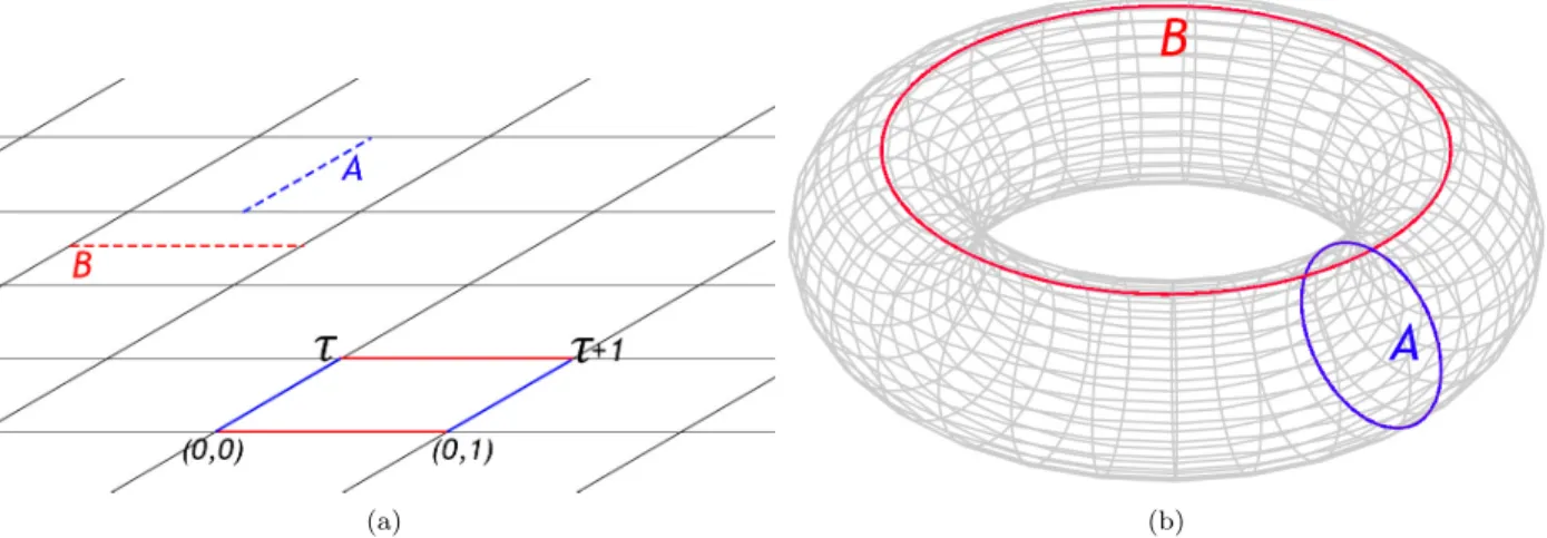
The Seiberg-Witten method is based on the effective action on the Coulomb branch of the theory. From the properties ofτ discussed at the beginning of this chapter, Seiberg and Witten realized that this moduli space is also where the modular transformations ofSL(2,Z) would be occurring; and that moduli space can be thought of as geometrically parameterized by the complex structure of aT2. ThisT2 can be written as the quotient space of the complex plane Cby a group denoted by h1, τiwhich ensures the periodicity of τ
(see Fig. 4.1a for visual depiction). This T2 =
C/h1, τispace then parameterizes elliptic curves described
by
y2=x3+f(u)x+g(u), (4.1)
where f and g are polynomials inu, and their exact form is decided by the flavor symmetry group Gflavor that we consider.
(a) (b)
Figure 4.1: (a). C/h1, τi plane. The lines of same color are considered equivalent, and thus construct the torus. The dashed lines are the “opened” version of cycles of the torus. (b). The torus created after connecting the equivalent lines of the C/h1, τi plane to each other. Loops A and B are the independent cycles of the torus.
space. (See Fig. 4.1b)
We can also define a modular invariant function for elliptic curves, called the Klein invariantj-function, as
j(τ) = 4f 3
4f3+ 27g2. (4.2)
Thej-function is only a function of the modular parameterτ and is therefore SL(2,Z) invariant. To avoid
SL(2,Z) redundancy, it is common to define a “fundamental domain” for the τ parameter and work only
in that domain. Mathematically, this domain is defined by H/SL(2,Z), where H = {Imτ > 0} is the
upper half plane. Geometrically, the domain is marked by the shaded area in Figure 4.2. All the values ofτ lying outside the fundamental domain can be mapped to a point inside the domain using anSL(2,Z) transformation. Additionally, whenτ is restricted to this domain, thej-function takes on every value in the complex planeCexactly once.
For a representationRofGflavor, we can then define theSeiberg-Witten (SW) differential,λR. According to [40] (which is in turn a review of [27]), the SW differential for a representationRcan be written as
λR= (c1u+c3B(u)) dx
y +c2 X
a
maya(u) x−xa(u)
dx
y , (4.3)
wherec1, c2andc3are normalization constants, andB(u) depends on the symmetry groupGflavor. For most smaller rank symmetry groups, B = 0. The sections (xa(u), ya(u)) are the poles of the SW differential, wherea= 1, ...,dimR, andma are the mass parameters at these poles.
Figure 4.2: The fundamental domain for the modular parameter τ is shaded in gray. Every point outside of this can be mapped into a point inside using anSL(2,Z) transformation, and the τ values inside of the domain give all the values in the complex planeCfor thej-function exactly once. This domain is restricted by conditions Imτ >0,−1
2 <Reτ ≤
1
2 and|τ| ≥1, which come fromH/SL(2,Z). The image is taken from Wikipedia.
and B loops of the torus, see Figure 4.1b
a= I
A
λR aD=
I
B
λR. (4.4)
In this setting,aandaD are called the SWperiods. An additional expression gives the mass parametersma around the poles
1 kR
ma 2√2 =
I
xa
λR.
Alternatively, the mass parameters for an irreducible representation R of Gflavor, can be found using the roots and weights ofGflavor. Define ~λa as the weight space vector of Rand~αf as the root space vector of
Gflavor. Then,
ma=~λa·ϕ~ (4.5)
whereϕ~ =P f~αfϕ
f, witha= 1, ...,dimRand f = 1, ...,rankGflavor.
At this point it is worth mentioning that knowledge of SW periods can also aid us in extracting the massM of BPS states introduced in Section 2.2.2. Indeed, assume a state has both electric and magnetic charges and is also charged under the flavor symmetry group. Let us denote these charges byqe, qm, andqa respectively. The central chargeZ of such a state would then be
Z =qmaD+qea+ 1
√
2 X
a
where a and aD are the SW periods, and the ma are the flavor symmetry characteristic mass parameters (4.5). The BPS mass is then given by
M =√2|Z|. (4.7)
Let us take a second look at eq. (4.6). The last term in (4.6) can be rewritten using the expression for mass parameters (4.5). We will have,
1
√
2 X
a
qama =√1
2 X
a
qa~λa·ϕ~
=√1
2 X
a qa~λa·
X
f ~ αfϕf
Now if we combine all the coefficients aswf, we can rewrite this as
1
√
2 X
f wfϕf
At this point we can define new “mass parameters”af as
af≡ √1
2ϕ f,
So that the overall BPS mass formula will become
M =√2qmaD+qea+ X
f wfaf
. (4.8)
The main benefit of writing the mass formula in this form is that it provides a very clear distinction and a straightforward understanding of the two types of coupling constants we investigate in this project. The
τextra, or τr+1,r+1 where r is the rank of the flavor symmetry group, which describes the coupling of the
extra sector with itself, and the so-calledτmix’s, which define the mixing between the extra sector and the flavor symmetry. In other words,
τmixf =τf,r+1≡ ∂a
D
∂af, forf = 1, ..., r τextra=τr+1,r+1≡ ∂a
D ∂a
whereris the rank of Gflavor.


![Figure 4.5: Graphs of components of coupling constant τ mix vs. mass parameter m, when u = 0.1 (orange) and u = 0.01 (blue), and mass parameter m takes over values from [0, 10] range](https://thumb-us.123doks.com/thumbv2/123dok_us/8324842.2207212/52.918.249.677.104.1060/figure-graphs-components-coupling-constant-parameter-parameter-values.webp)