INTEGRATING OPTIMIZATION AND SAMPLING FOR ROBOT MOTION PLANNING WITH APPLICATIONS IN HEALTHCARE
Alan Kuntz
A dissertation submitted to the faculty at the University of North Carolina at Chapel Hill in partial fulfillment of the requirements for the degree of Doctor of Philosophy in the Department of
Computer Science in the College of Arts and Sciences.
Chapel Hill 2019
c 2019 Alan Kuntz
ABSTRACT
Alan Kuntz: Integrating Optimization and Sampling for Robot Motion Planning with Applications in Healthcare
(Under the direction of Ron Alterovitz)
Robots deployed in human-centric environments, such as a person’s home in a home-assistance setting or inside a person’s body in a surgical setting, have the potential to have a large, positive impact on human quality of life. However, for robots to operate in such environments they must be able to move efficiently while avoiding colliding with obstacles such as objects in the person’s home or sensitive anatomical structures in the person’s body. Robot motion planning aims to compute safe and efficient motions for robots that avoid obstacles, but home assistance and surgical robots come with unique challenges that can make this difficult. For instance, many state of the art surgical robots have computationally expensive kinematic models, i.e., it can be computationally expensive to predict their shape as they move. Some of these robots have hybrid dynamics, i.e., they consist of multiple stages that behave differently. Additionally, it can be difficult to plan motions for robots while leveraging real-world sensor data, such as point clouds.
ACKNOWLEDGEMENTS
First, I would like to thank my graduate advisor, Ron Alterovitz, for his invaluable support and guidance in matters both technical and otherwise throughout my time in graduate school. I would like to thank my undergraduate advisor, Lydia Tapia, for encouraging me to pursue a graduate education and setting me up for success as I continue my career. I would also like to thank my committee members for their valuable time, guidance, support, and feedback.
Next, I would like to thank the other students with whom I’ve shared a lab, offices, and the graduate experience. Specifically, I would not have been successful without the mentorship of Luis Torres, Jeff Ichnowski, Chris Bowen, and Kasra Manavi.
This work was made possible by the National Science Foundation (NSF) under awards IIS-1149965, CNS-1305286, and CCF-1533844, and the National Institutes of Health (NIH) under awards R21EB017952 and R01EB024864.
TABLE OF CONTENTS
LIST OF FIGURES . . . xi
LIST OF TABLES . . . xiii
CHAPTER 1: INTRODUCTION . . . 1
1.1 Challenges . . . 2
1.2 Contributions . . . 4
1.2.1 Motion Planning for Continuum Reconfigurable Incisionless Surgical Parallel Robots . . . 4
1.2.2 Kinematic Design Optimization of a Parallel Surgical Robot to Maximize Anatomical Visibility via Motion Planning . . . 5
1.2.3 Motion Planning for a Three-Stage Multilumen Transoral Lung Access System 5 1.2.4 Toward Transoral Peripheral Lung Access: Steering Bronchoscope-Deployed Needles through Porcine Lung Tissue . . . 6
1.2.5 Fast Anytime Motion Planning in Point Clouds by Interleaving Sampling and Interior Point Optimization . . . 6
1.2.6 Planning High-Quality Motions for Concentric Tube Robots in Point Clouds via Parallel Sampling and Optimization . . . 6
1.2.7 Estimating the Complete Shape of Concentric Tube Robots via Learning . . . 7
1.3 Thesis Statement . . . 8
1.4 Organization . . . 8
CHAPTER 2: MOTION PLANNING FOR CONTINUUM RECONFIGURABLE INCISIONLESS SURGICAL PARALLEL ROBOTS . . . 9
2.1 Related Work . . . 11
2.2 Problem Formulation . . . 12
2.2.1 CRISP Robot . . . 12
2.2.2 Motion Planning . . . 13
2.3.1 Motion Planning . . . 14
2.3.2 Mechanics & Solution Seeding . . . 16
2.3.3 Candidate CRISP Setup Evaluation . . . 19
2.4 Results . . . 19
2.4.1 Generating Visibility Sets . . . 20
2.4.2 Motion Planning to View a Specific Goal Point . . . 22
2.4.3 Mechanics Solution Seeding . . . 22
2.5 Conclusion . . . 23
CHAPTER 3: KINEMATIC DESIGN OPTIMIZATION OF A PARALLEL SURGICAL ROBOT TO MAXIMIZE ANATOMICAL VISIBILITY VIA MOTION PLANNING . . . 25
3.1 Related Work . . . 27
3.2 Problem Definition . . . 29
3.2.1 Design Space . . . 29
3.2.2 Configuration Space . . . 30
3.2.3 Workspace . . . 30
3.2.4 Maximizing Viewable Anatomy . . . 31
3.3 Method . . . 31
3.3.1 Exploring Design Space . . . 33
3.3.2 Evaluating Candidate Designs . . . 33
3.4 Analysis . . . 35
3.4.1 Preliminaries . . . 35
3.4.2 Sampling Optimal Designs Infinitely Often . . . 36
3.4.3 Asymptotic Optimality . . . 38
3.5 Results . . . 38
3.6 Conclusion . . . 40
CHAPTER 4: MOTION PLANNING FOR A THREE-STAGE MULTILUMEN TRANSORAL LUNG ACCESS SYSTEM . . . 43
4.1 Related Work . . . 45
4.3 Method . . . 49
4.3.1 Planning Deployment of the Bronchoscope . . . 50
4.3.2 Planning Deployment of the Concentric Tube Robot . . . 51
4.3.3 Steering the Bevel-Tip Needle to the Goal Point . . . 51
4.3.4 Motion Planning for the Entire System . . . 53
4.4 Results . . . 53
4.5 Conclusion . . . 56
CHAPTER 5: TOWARD TRANSORAL PERIPHERAL LUNG ACCESS: STEERING BRONCHOSCOPE-DEPLOYED NEEDLES THROUGH PORCINE LUNG TISSUE . . . 57
5.1 Materials & Methods . . . 57
5.2 Results . . . 59
5.3 Discussion . . . 60
CHAPTER 6: FAST ANYTIME MOTION PLANNING IN POINT CLOUDS BY INTERLEAVING SAMPLING AND INTERIOR POINT OPTIMIZATION . 62 6.1 Related Work . . . 65
6.2 Problem Definition . . . 66
6.3 Method . . . 67
6.3.1 Global Exploration using Sampling-Based Motion Planning . . . 68
6.3.2 Lazy Interior Point Optimization . . . 69
6.3.3 Asymptotic Optimality . . . 73
6.4 Results . . . 73
6.4.1 Motion Planning for a 3D Spherical Robot . . . 75
6.4.2 Motion Planning for the Arm of a Baxter Robot . . . 76
6.5 Conclusion . . . 80
CHAPTER 7: PLANNING HIGH-QUALITY MOTIONS FOR CONCENTRIC TUBE ROBOTS IN POINT CLOUDS VIA PARALLEL SAMPLING AND OPTIMIZATION . . . 81
7.1 Related Work . . . 84
7.2 Problem Definition . . . 86
7.3.1 Method Overview . . . 88
7.3.2 Global Exploration through Sampling . . . 89
7.3.3 Interior Point Local Optimization . . . 90
7.3.4 Keeping Track of the Best Plan Found . . . 91
7.4 Results . . . 92
7.4.1 Comparison and Analysis . . . 93
7.4.2 Adapting to Changing Anatomy . . . 95
7.5 Conclusion . . . 97
CHAPTER 8: ESTIMATING THE COMPLETE SHAPE OF CONCENTRIC TUBE ROBOTS VIA LEARNING . . . 98
8.1 Materials & Methods . . . 99
8.2 Results . . . 101
8.3 Discussion . . . 103
CHAPTER 9: CONCLUSION . . . 104
LIST OF FIGURES
1.1 Examples of robotic systems that may be used in a healthcare setting . . . 2
2.1 CRISP system and motion planning framework overview . . . 10
2.2 CRISP parameter diagram . . . 13
2.3 Segmented pleural effusion volume in anatomical setting . . . 20
2.4 Two setups for the CRISP robot . . . 21
2.5 Visibility sets for each setup . . . 21
2.6 Percentage of goal points seen . . . 22
2.7 An example CRISP motion plan . . . 23
3.1 Two images of the CRISP robot . . . 26
3.2 2D example of the impact of different designs . . . 27
3.3 The CRISP robot’s kinematic design parameters . . . 30
3.4 Scenario 1 . . . 39
3.5 Scenario 2 . . . 40
3.6 Percent viewed over time for each scenario . . . 41
3.7 Anatomy visualized at 2 minutes and at 8 hours . . . 41
4.1 Example motion plan for three-stage robot . . . 44
4.2 The three stages . . . 45
4.3 Utilizing different branches of bronchial tree . . . 50
4.4 Trunpet-shaped reachable workspace of the steerable needle . . . 52
4.5 Safe bronchoscope deploy positions . . . 54
4.6 First 15 solutions across multiple homotopic classes . . . 54
4.7 Lung nodule query locations . . . 55
4.8 Percentage of lung nodules successfully planned to . . . 55
4.9 Path cost over time . . . 56
5.1 System deployed in inflated ex vivo porcine lung in CT scanner . . . 58
5.3 Segmentation and path from CT scan . . . 60
5.4 CT scan slices of deployment . . . 61
6.1 Overview of ISIMP . . . 64
6.2 Lazy constraint set use overview . . . 71
6.3 Cutoff function and bisection overview . . . 73
6.4 3D point cloud environment . . . 74
6.5 3D cost over time with varying point cloud sizes . . . 74
6.6 Comparison to sampling-based methods . . . 77
6.7 Comparison to optimization-based methods . . . 78
6.8 Visualization of baxter results . . . 79
7.1 PSIMP overview . . . 82
7.2 Concentric tube robot moving through different homotopy classes in point cloud . . . 84
7.3 Examples of plans before and after optimization . . . 89
7.4 Point clouds from real patient anatomy . . . 92
7.5 Ratio to best plan over time . . . 94
7.6 Direct comparison over time . . . 95
7.7 Point cloud representation of modified anatomy enables new motions . . . 96
8.1 Learned concentric tube model diagram . . . 99
8.2 Shape from silhouette setup . . . 100
LIST OF TABLES
5.1 Needle steering tip errors in porcine lung . . . 60
6.1 Statistics on point cloud points used by ISIMP . . . 76
8.1 Polynomial basis function coefficients . . . 101
8.2 Tube parameters for the 3-tube concentric tube robot . . . 101
CHAPTER 1 Introduction
In order for robots to have a large, positive impact on human quality of life, they must be able to safely and effectively operate in human-centric environments. One area in which robots have a large potential for positive impact is healthcare. Robots have the potential to assist people in their homes with tasks that these people may be unable to perform themselves due to age, disease, disability, or other factors. Robots in a surgical setting have the potential to increase the capabilities of surgeons, enabling the surgeons to perform new or existing procedures more safely and on a larger class of patients than is currently possible.
In both of these human-centric settings, robots must be capable of operating safely, avoiding unintentional collisions with obstacles in their environments. In a home assistance setting, the obstacles a robot must avoid may be the humans or objects in the humans’ home. In a surgical setting, the obstacles may be inside the humans themselves—anatomical obstacles, such as bones, nerve bundles, or vasculature. In addition to avoiding unintended collision with obstacles, the robots must be effective at performing the tasks required of them. One approach to enabling robots to operate in a safe and effective manner in human-centric environments isrobot motion planning.
Robot motion planning methods compute motions for a robot to perform a user-specified task subject to a set of constraints. These constraints can be problem and robot specific, and frequently include kinematic constraints (such as joint limits), differential constraints (such as a minimum turning radius along the robot’s path), and environmental constraints (such as obstacle avoidance described above). Then, under a set of assumptions (such as perfect modeling and knowledge of the environment), any computed motion that satisfies these constraints is known to be safe, as it does not collide with the environment, as well as feasible, i.e., it conforms to the robot’s kinematic requirements.
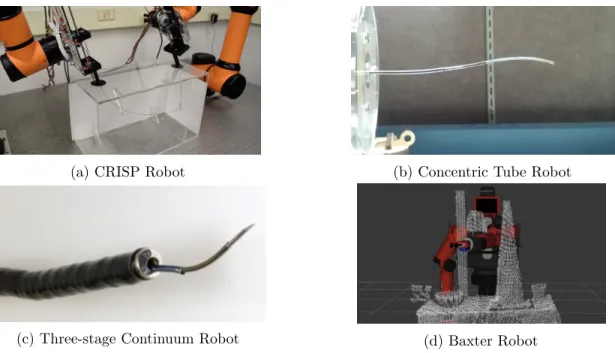
(a) CRISP Robot (b) Concentric Tube Robot
(c) Three-stage Continuum Robot (d) Baxter Robot
Figure 1.1: We plan safe and effective motions for a variety of different types of robots, including those shown here. (a) The Continuum Reconfigurable Incisionless Surgical Parallel (CRISP) robot is composed of multiple needle-diameter tubes that are assembled into a parallel structure using snares [1, 2]. (b) A concentric tube robot is composed of multiple telescoping precurved flexible tubes [3, 4]. (c) A three-stage continuum robot combines a tendon-actuated bronchoscope with concentric tubes and a steerable needle [5]. (d) A Baxter robot is a commercially available robot with two 7 degree of freedom (DOF) serial-link manipulator arms [6].
motion plan. A high-quality plan under such a metric would ensure that the plan avoids unnecessary motion, reducing the time and energy spent by the robot to execute the task. Another relevant cost metric is clearance from obstacles, wherein a high-quality plan would travel far from the obstacles in the environment, improving the safety of the plan as it is executed.
In this dissertation, we present and evaluate novel algorithms that compute safe (constraint satisfying) and effective (high-quality) motion plans for robots, such as those shown in Fig. 1.1, in healthcare applications. In order to do so, our methods leverage a combination of sampling- and optimization-based methods.
1.1 Challenges
Computationally expensive kinematic models One class of robot that we focus on is contin-uum surgical robots. Contincontin-uum surgical robots are robots that are capable of taking curved shapes which allow them to safely travel deep into the human body [7], enabling minimally invasive surgical procedures (for examples of such systems, see Figs. 1.1a, 1.1b, and 1.1c). Successfully planning motions for such systems will allow for less invasive surgical procedures as they curve around sensitive anatomical structures. However, computing the anticipated shape of continuum surgical robots frequently takes orders of magnitude longer than computing the shape of traditional robotic systems such as serial-link manipulators [4, 8]. This limitation must be addressed for motion planning to be successful for such systems.
Parameters set pre-procedure which greatly impact capabilities For systems such as the Continuum Reconfigurable Incisionless Surgical Parallel (CRISP) robot (see Fig. 1.1a), decisions are made prior to the surgical procedure such as where on the patient’s body the robot is inserted and the robot’s parallel structure. We refer to these parameters as the robot’s kinematic design. Decisions about the robot’s kinematic design are frequently made heuristically and can have a large impact on the success of the surgical procedure.
Hybrid and highly-constrained kinematics in multistage robots The 3-stage robot shown in Fig. 1.1c consists of multiple robotic stages that are deployed in sequence and that all behave differently. Some of these stages are holonomic, while others are non-holonomic, making it difficult to efficiently integrate the stages into a single motion planning framework. Additionally, decisions made when planning motions for each of the stages dramatically impacts the stages that are deployed later in time. This property must be accounted for when planning motions for such hybrid systems.
environments can be difficult due to the large number of points and their lack of inherent structure.
Inaccurate shape models For some continuum robot systems, such as concentric tube robots (see Fig. 1.1b) the physics-based shape models may be inaccurate due to issues such as material inhomogeneities and inconsistent and difficult to predict physical phenomena such as friction [9, 10]. Motion planning and control of these systems rely on the assumption that the shape model is accurate.
1.2 Contributions
Many methods have already been developed for planning motions for a variety of robots. However, these methods frequently do not work well in the presence of the challenges described above. As such, in this work we adapt, integrate, and develop novel algorithms specifically to address the above challenges as we plan motions for these systems. We discuss our methods briefly here and in full detail in the corresponding chapters.
1.2.1 Motion Planning for Continuum Reconfigurable Incisionless Surgical Parallel Robots
1.2.2 Kinematic Design Optimization of a Parallel Surgical Robot to Maximize Anatomical Visibility via Motion Planning
In order to address the challenge of effectively setting pre-procedure parameters, we introduce a method to optimize, on a patient-specific basis, the kinematic design of the CRISP robot. Our objective is to maximize the ability of the robot’s tip camera to view tissue surfaces in constrained spaces. The kinematic design of the CRISP robot, which greatly influences its ability to perform a task, includes parameters that are fixed before the procedure begins, such as entry points into the body and parallel structure connection points. We combine a global stochastic optimization algorithm, Adaptive Simulated Annealing (ASA), with the motion planner designed for the CRISP robot. ASA facilitates exploration of the robot’s design space while the motion planner enables evaluation of candidate designs based on their ability to successfully view target regions on a tissue surface. By leveraging motion planning, we ensure that the evaluation of a design only considers motions which do not collide with the patient’s anatomy. We analytically show that the method asymptotically converges to a globally optimal solution and demonstrate our algorithm’s ability to optimize kinematic designs of the CRISP robot on a patient-specific basis. This contribution is discussed in Chapter 3 and was presented in [11].
1.2.4 Toward Transoral Peripheral Lung Access: Steering Bronchoscope-Deployed Needles through Porcine Lung Tissue
In this work, we physically deploy and evaluate the efficacy of the three-stage lung tumor biopsy robot in biological tissue. We deploy the robot into inflated porcine lung and demonstrate the robot’s ability to steer around anatomical obstacles to targets in the periphery of the lung with high accuracy. We run a number of trials in the lung achieving average needle-tip errors in the1mm to2
mm range. We also gather CT scans of the robot’s deployment in the lung to visualize the robot’s placement in the anatomy. This contribution is discussed in Chapter 5 and was originally presented in [13].
1.2.5 Fast Anytime Motion Planning in Point Clouds by Interleaving Sampling and Interior Point Optimization
Robot manipulators operating in unstructured environments, such as in home assistance settings, need to plan their motions quickly while relying on real-world sensors, which typically produce point clouds. To enable intuitive, interactive, and reactive user interfaces, the motion plan computation should provide high-quality solutions quickly and in an anytime manner, meaning the algorithm progressively improves its solution and can be interrupted at any time and return a valid solution. To address these challenges, we combine two paradigms: (1) asymptotically-optimal sampling-based motion planning, which is effective at providing anytime solutions but can struggle to quickly converge to high quality solutions in high dimensional configuration spaces, and (2) optimization, which locally refines paths quickly. We propose the use of interior point optimization for its ability to perform in an anytime manner that guarantees obstacle avoidance in each iteration, and we provide a novel lazy formulation that efficiently operates directly on point cloud data. Our method iteratively alternates between anytime sampling-based motion planning and anytime, lazy interior point optimization to compute high quality motion plans quickly, converging to a globally optimal solution. This contribution is discussed in Chapter 6 and was originally presented in [14].
1.2.6 Planning High-Quality Motions for Concentric Tube Robots in Point Clouds via Parallel Sampling and Optimization
surgery. As in the previous contribution, our motion planning method uses a combination of sampling-based motion planning methods and local optimization, via an interior point method, to efficiently handle point cloud data and quickly compute high quality plans. This ensures that the computed plan is feasible and avoids obstacles at every iteration, in an anytime fashion. Building upon the previous contribution, rather than interleaving the sampling- and optimization-based methods we instead present a framework that leverages parallelism to efficiently do both simultaneously. Additionally, rather than minimizing the motion plan’s length, we instead minimize a cost metric that encourages clearance from obstacles, promoting safer motion plans. We demonstrate the method’s efficacy in three anatomical scenarios, including two generated from endoscopic videos of real patient anatomy. This contribution is discussed in Chapter 7 and will appear in [15].
1.2.7 Estimating the Complete Shape of Concentric Tube Robots via Learning In order to successfully plan motions for concentric tube robots, the motion planner needs to be able to accurately determine the shape of the robot as it moves through the world. Traditionally, this is done using physics-based mechanical models that are based on complex mechanical concepts such as Cosserat rod theory. However, these models have difficulty accurately accounting for all of the complex physical phenomenon associated with the robot in the real world, such as friction between the tubes. As a result, the mechanical models are frequently inaccurate. We propose a data-driven, machine learning based approach using a deep neural network to solve this problem.
1.3 Thesis Statement
This dissertation proposes the following thesis:
For robots operating in human-centric environments, robot motion planning, via a combination of sampling- and optimization-based methods, enables fast and high-quality kinematic design optimization and motion computation while overcoming challenges associated with computationally expensive kinematic models, hybrid and highly-constrained kinematics, and point-cloud obstacle representations.
Each chapter of this dissertation supports this thesis statement as outlined below. 1.4 Organization
CHAPTER 2
Motion Planning for Continuum Reconfigurable Incisionless Surgical Parallel Robots
The Continuum Reconfigurable Incisionless Surgical Parallel (CRISP) robot [1] is a new type of continuum robot [7, 19] that consists of multiple needle-diameter flexible instruments that are assembled together inside a body cavity to perform minimally invasive medical procedures. The CRISP robot typically includes (1) a flexible instrument with a working channel through which a tool (e.g., chip-tip camera, ablation probe, etc.) is passed, and (2) one or more additional flexible instruments that are inserted into the body cavity and attach to the first instrument via snares, creating a strong, parallel kinematic structure (see Fig. 2.1). The parallel nature of the structure provides strength to the robot, enabling the device to apply larger forces during medical procedures when required. The tool’s tip can be repositioned and reoriented inside the body by robotically moving the instruments outside the body in concert.
The CRISP robot is an ideal platform for inspecting and manipulating tissues on the surface of a pleural effusion, which is a collection of excess fluid in the pleural space around the lungs. Pleural effusions can be caused by over 50 different diseases [20]. Accurate diagnosis of the disease is critical, as the underlying cause can be deadly and may have drastically different treatment paths. Thoracoscopy is the gold standard and involves insertion of endoscopic tools through the ribs [21]. Endoscopic tools give clinicians direct visualization of the pleural space. However, thoracoscopy is invasive: it requires incisions, and major complications are reported to be as high as 15% [22]. A CRISP robot, with a chip-tip camera deployed through the tool working channel, has the potential to combine the minimal invasiveness of needles with the ability of endoscopic tools to systematically inspect the interior surface of a patient’s pleural effusion.
RCM
obstacle chip-tip
camera
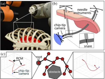
Figure 2.1: An overview of the CRISP robotic system and motion planning framework. (a) The needle-diameter flexible instruments form a parallel structure inside the body whose shape is modified by actuating the instruments outside the body. (b) The instruments can be inserted and rotated to change the view of the camera at the tip. (c) The motion planner incrementally computes a tree data structure of collision-free robot configurations, which can be used to manipulate the instruments (shown in red) outside the body to reposition and reorient the camera tip while ensuring the instruments avoid anatomical obstacles inside the body.
the body avoid collision with anatomical obstacles, including the chest wall, the lung surface, and potential connections between the lung and chest wall. The configuration of the CRISP robot is the position and orientation of the instruments outside the body, and the motion planner computes a sequence of configurations that avoids collisions with anatomical obstacles inside the body, enforces remote-center-of-motion constraints on the tube’s entry points into the body, and enables visibility of the desired clinical site inside the body with the tool’s camera. Motion planning for CRISP robots is challenging because evaluating their kinematics for each configuration requires modeling the elastic and torsional interactions of the robot’s constituent tubes, which is computationally expensive. We introduce a sampling-based motion planner that efficiently propagates presolved state information for the kinematic model through a tree data structure in configuration space to accelerate motion plan computation.
estimate the set of points on the pleural effusion surface that can be seen by the tool tip camera of a CRISP robot for a given setup, as well as provide collision free motion plans for the robot to view the points on the pleural effusion surface. This analysis can provide physicians with insights into CRISP robot setups that are appropriate for specific clinical tasks that require pointing the camera at specific sites in the pleural effusion.
We demonstrate the speed and effectiveness of our new motion planner for CRISP robots in simulation using a pleural effusion segmented from a patient CT scan. We demonstrate both the method’s ability to plan motions for the robot to view specific clinically relevant sites as well as the ability to estimate the set of points that can be seen by the CRISP robot’s tool tip camera.
This chapter is based on work previously published in [8].
2.1 Related Work
Motion planning for the CRISP robot [1] is influenced by the way the shape of the robot is calculated. This influence is not unique to the CRISP robot and is a consideration present in motion planning for other continuum surgical robots.
One continuum surgical robot with related mechanics is the concentric tube robot [23]. Concentric tube robots are needle-like surgical manipulators composed of thin, nested, pre-curved nitinol tubes. Similar to the mechanics of the CRISP robot, the tubes of the concentric tube robot elastically interact in different configurations to influence the robot’s shape. Using various control methods, prior work has achieved position control of concentric tube robot tips [24, 9, 25]. Sampling based motion planning has also been used to control concentric tube robots. Torres et. al. use a combination of a precomputed roadmap and an inverse kinematics controller to achieve interactive rate planning for concentric tube robots [4]. Lyons et. al. apply optimization-based motion planning using a simplified kinematics model [26].
Another related medical robotic device for interventional medical procedures is steerable needles, which are composed of a highly flexible tube and employ an asymmetric tip to steer through soft tissue [27]. Motion planning for steerable needles has been achieved in a variety of ways [28, 29, 30], including sampling-based motion planning [31, 32, 12].
in the lung through the airway [34] but are restricted in their motion to the structure of the bronchial tree. In non-medical applications, probabilistic roadmaps have been applied to plan camera paths in virtual environments when given a specified goal position and orientation for the camera [35]. There has also been work in computer vision on how to plan new viewpoints for a camera such that object recognition is optimized [36, 37]. These works primarily consider how to plan the viewing angles of the camera, while we primarily focus on motion planning for a medical robot that contains a camera for purposes of viewing specific sites in cluttered and constrained spaces.
2.2 Problem Formulation
2.2.1 CRISP Robot
We consider a CRISP robot composed of N needle-diameter tubes. One of these tubes has a chip-tip camera affixed to its tip which we refer to as the camera tube,ρc. The remainingN−1tubes
are deployed with snares, and will be referred to as snare tubes,ρk, wherekis an integer uniquely
identifying a specific snare tube. In order to perform accurate mechanical modeling, we require as input each tube’s inner diameter (ID) and outer diameter (OD). We also require a description of the chip-tip camera, in the form of its angular field of view,θv.
A CRISP robot’s set of tubes can be assembled into parallel structures inside the patient’s body in an infinite number of ways. We require as input a description of the CRISP robot state (illustrated in Fig. 2.2). We make a distinction between the CRISP robot’ssetup state and the robot’sactuatable state. We define the CRISP robot’ssetup state as:
{rc,r1, . . . ,rN−1, s1, . . . , sN−1}, (2.1)
where rc ∈ R3 and rk ∈ R3, k = 1, . . . , N −1 denotes the tubes’ entry points into the patient’s
body, expressed in a global coordinate system, and the scalars sk denote the arc length along the
camera tube at which the kth snare tube attaches to the camera tube. The subscript c denotes a value corresponding to the camera tube, and an integer k denotes the value corresponding to thekth snare tube. This setup state is set prior to the surgical procedure and is not varied during
x
1
x
2
x
c
l
1
l
2
s
1
s
2
r
c
r
1
r
2
l
c
field of view chip-tip
camera flexible
instruments body entry points stiff outer
sheaths
snare grasp point
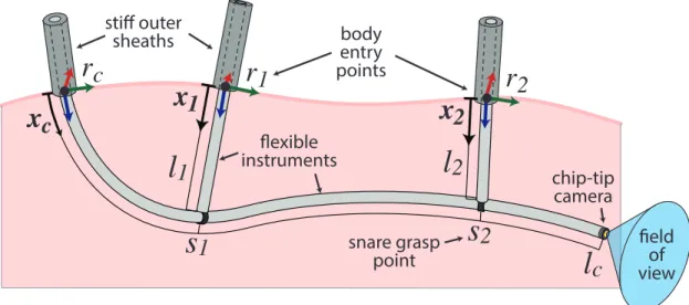
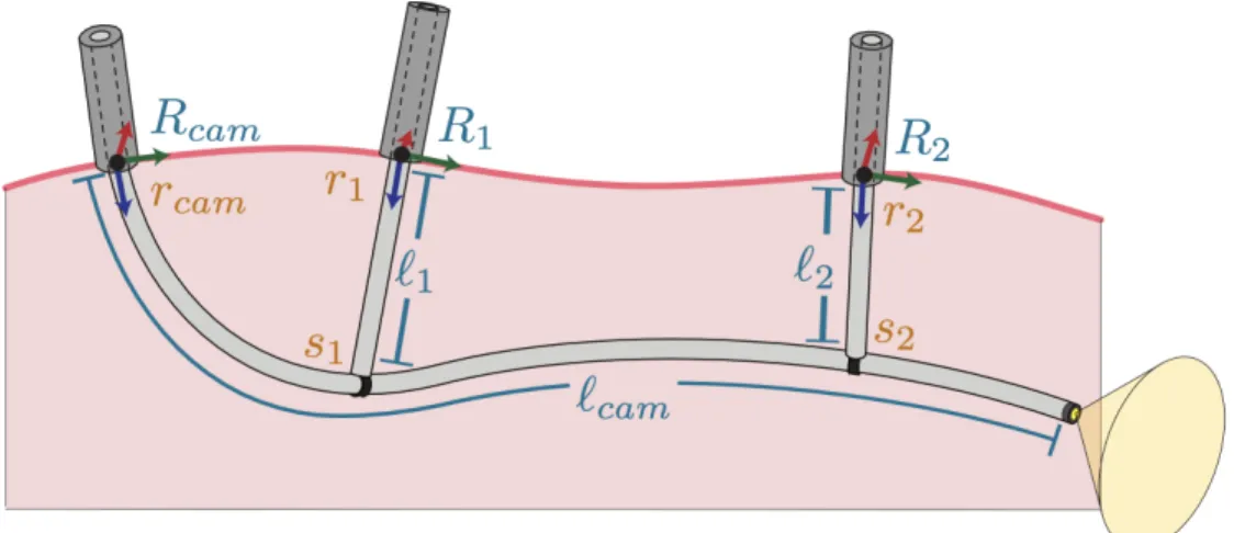
Figure 2.2: A stiff outer sheath introduces the tubes into the body entry pointsrc, r1, and r2. The
snares grasp the camera tube at arc lengthss1 ands2. A mechanics-based model predicts the states
of the camera tubexc and the snare tubes, x1 and x2, in arc length.
CRISP robot’s actuatable state as:
{Rc, R1, . . . , RN−1, `c, `1, . . . , `N−1}, (2.2)
where R ∈ SO(3) denotes the tubes’ orientations at their entry points as expressed in a global coordinate system, and the scalars`describe how far each of the tubes are inserted beyond their respective entry points into the body (with a maximum insertion length for each tube imposed by the physical robot). Thisactuatable state represents the robot’s state which will be varied during the execution of motions during the surgical procedure. The CRISP robot’s total state then becomes the union of the setup and actuatable states.
2.2.2 Motion Planning
We consider the problem of planning motions for a CRISP robot. To produce motion, each tube can be actuated via changing its orientation at the entry point into the pleural effusion space and translating the tube into and out of the space.
We define an instance of the robot’s actuatable state as a configuration
The space of all configurations the robot can assume is then Q⊆ SO(3)N ×RN.
For a given configuration q∈Qwe define the shape of the CRISP robot as a function
P(q, ρ, s) :SO(3)N ×RN × N ×R7→R3.
Function Pis a 3D space curve representing the backbone of tubeρ, at arc lengthsin the domain
[0, lρmax]. FunctionP, combined with knowledge of the cross-sectional outer diameter (OD) of each
tube allows us to calculate the shape of the entire CRISP robot. Also note, that as a special case,
pcamera is the 3D location of the camera on the tip of ρc, and it has a direction of view defined by
the vector vcamerawhich is tangent to the space curve at pcamera.
We then define a motion planσ= (q0,q1, . . . ,qn)as an ordered sequence of robot configurations.
We define a collision free plan as a plan for which the shape of the robot at every configuration in the plan does not collide with obstacles in the environment, and an interpolation between adjacent configurations does not collide with obstacles in the environment. We then define a valid plan as a plan that is collision free and achievable given the robot hardware.
When computing a motion plan, our method takes as input a CRISP setup, an initial configuration
q0, a Computed Tomography (CT) scan from which we will define the environment, and a goal point pgoal, the location in the anatomy that the physician is attempting to view with the camera. Our
method then produces as output a planσ, which is a collision-free sequence of configurations that will result in the robot being able to view pgoal.
When evaluating the quality of a candidate setup, we require as input the setup, an initial configuration q0, and the CT scan. Then, instead of outputting a plan to a specific goal point, we
instead output a set of cells on the interior surface of the pleural effusion which can be seen by manipulation of the CRISP robot with that specific setup, which we define as a visibility set.
2.3 Method
2.3.1 Motion Planning
To model the environment for our motion planner, we use an occupancy grid. The grid has free cells, Sfree, in which the robot is allowed to freely move, and occupied cells,Sobs, which the motion
We setSfree to be the cells in the CT scan consistent with the pleural effusion andSobs to be the
inverse segmentation. We also define a third set, Sbound to be the cells in Sobs which are adjacent
toSfree which will contain the goal point of interestpgoal and which will be the set we attempt to
visualize in the evaluation of a setup.
We solve the motion planning problem formulated in Sec. 2.2.2 using a sampling-based approach. We implement a planner based on the Rapidly-Exploring Random Trees (RRT) method [39]. The RRT method begins at a root node, the initial configuration, and iteratively and randomly constructs a tree structure where each node in the tree is a valid configuration, and an edge linking two nodes is a valid, collision free motion between them as a linear interpolation in configuration space. As the tree grows, it expands and explores the obstacle free configuration space of the robot. Once a node is found which has a camera pose with a clear view of the goal point, pgoal in the lung, the
tree can be traced back to the root node, and a valid plan from the initial configuration to a goal configuration has been found.
Specifically, we begin with our root node. We then sample a randomly generated point in configuration space. We linearly interpolate between the two configurations, using spherical linear interpolation (SLERP) [40] to interpolate between the rotational degrees of freedom. We then propagate along the line segment starting at the root node for a random percentage of the line segment, computing the shape of the robot and checking it againstSobs at a fine discretization. If the
robot collides with obstacles or reaches a configuration that the forward kinematics solver is unable to solve, we stop at the prior step of the discretization. We then add the last valid configuration and edge to the tree. This process is then repeated, but the node from which to start the propagation is chosen as the nearest neighbor in the tree to the newly sampled point.
This process continues until a time limit has passed or until a configuration has an unobstructed view ofpgoal, whichever comes first.
occupy, and doing an index lookup into the CT-derived occupancy grid for those cells.
To identify whether at a sampled configuration pgoal is visible from the camera on the tip of
ρc we implement a ray trace. First, the camera position and direction of view, pcamera and vcamera
are inferred from the tip of the shape computed for ρc. The vector between pgoal and pcamera is
computed, and it is compared with vcamera. To identify ifpgoallies within the field of view of the
camera, we examine the planar angle between the two vectors. If the angle is larger than θv/2, then pgoal does not lie within the field of view of the camera. If, however, the angle is less thanθv/2, then pgoal does lie in the field of view of the camera. This is not enough, however, because there must
exist line of sight between the camera andpgoal—the view ofpgoalmay be occluded by another part
of the patient anatomy. To identify if there exists clear line of site, a ray is traced frompcamerato pgoal. If the ray strikes an occupied cell in Sobs before it reaches pgoal, there is not clear line of site
and the motion planning continues. However, if there exists clear line of site then the plan is traced back to the root initial configuration and is returned.
2.3.2 Mechanics & Solution Seeding
One of the most computationally intensive aspects of the method is computing the forward kinematics of the CRISP robot that determines its shape. This is done for every node in the tree, and at every finely discretized point along each edge in the tree. The forward kinematics is calculated both to ensure the configuration is collision free everywhere on the CRISP robot’s body and to identify the camera pose.
The forward kinematics of the CRISP robot results from its mechanics, which were initially presented in [1]. In this chapter, we assume that the flexible instruments of a CRISP robot can be physically held by robot manipulators at the point where the tubes enter the patient’s body. This reduces the dimensionality of the CRISP robot’s actuation space to only include orientation of each tube at the body entry point and each tubes’ insertion length into the body. This assumption also simplifies the system mechanics and can be physically implemented in practice using stiff introducer sheaths through which the flexible instruments can be deployed. What follows is a summary of the simplified CRISP robot’s mechanics and forward kinematics.
We model the CRISP robot using the Cosserat rod equations [41, 42], which define a system of ordinary differential equations that govern the Cosserat-rod state of each tube. This state consists
momentm∈R3, and internal forcen∈
R3 of each tube, each as a function of arc length along the
tube’s backbone. For instance, the Cosserat-rod state of the camera tube is defined as
xc(s) = [pc(s) Rc(s) mc(s) nc(s)], 0≤s≤`c, (2.3)
wheresis the arc length parameter and`c is the length of the camera tube. We define the
Cosserat-rod state of the snare tubes,xk(s) for the kth snare tube, similarly. For more details on Cosserat
rod theory, we direct the reader to [41] and [42].
The forward kinematics of a multi-tube system are formulated as a multi-point boundary value differential equation, where the Cosserat-rod states of thekthsnare tube propagate along its backbone
in arc length 0≤s≤`k as
x0k(s) =
[p0k(s) Rk0(s) m0k(s) n0k(s)], sk−`k ≤s≤sk
0, otherwise
, (2.4)
where sk is the grasp location of thekth snare tube. The states of the camera tube propagate along
its backbone in arc length0≤s≤`c, as
x0c(s) =
[p0c(s) Rc0(s) m0c(s) +α n0c(s) +β], 0≤s≤`c
0, otherwise
, (2.5)
where0 denotes the derivative with respect to arc length. These derivatives, as well as the termsα and β, can be found in [1]. The tube lengths (`c and`k) and the initial values of the tube position
(pk(0) and pc(0)) and orientation (Rk(0) and Rc(0)) at the body entry points are given by the
corresponding entry point position and orientation from the starting state, (2.1) and (2.2). The initial values of the Cosserat-rod internal moments (mk(0)andmc(0) ) and forces (nk(0)andnk(0))
for both the snare and camera tubes are determined later to satisfy the constraints of the multi-point boundary value problem.
The constraints of the multi-point boundary value problem include a constraint at each of the grasp pointssk on the camera tube’s body. The grasp constraints enforce the tip position of the
snare tube is constrained so that there is a constant rigid body rotation that maps the snare tip orientation to the backbone pose of the camera tube’s orientation at arc length sk as
ck =
pk(`k)−pc(sk)
RTc(sk)Rk(`k)Rx−I
=0 (2.6)
where Rx ∈SO(3) is the rotation in the [−1,0,0]T direction by 90◦ and I ∈R3×3 is the identity
matrix.
Under the assumption that the system is quasistatic and in the absence of applied forces and moments at the camera tube’s tip, the force and moment at the camera tube’s tip will be zero, leading to the additional constraint of
cc(`c) =
mc(`c)
nc(`c)
=0. (2.7)
TheN −1 grasp constraintsci and the tip constraintcc can be packed into the total constraint
vector
c=
cc c1 . . . cN−1
=0. (2.8)
The multi-point boundary value problem is solved by varying the snare and camera tube’s initial conditions of their moments (mk(0) and mc(0) ) and forces (nk(0) and nc(0)) so that the total
constraint equation (2.8) is satisfied. When solved, the multi-point boundary value problem yields the system’s forward kinematics. We accomplish this using a numerical optimization routine known as a “shooting” method, where an initial seed of the snare and camera tube’s initial internal moment are iteratively perturbed to minimize kck [1].
The runtime of the forward kinematics computation is heavily dependent on the initial conditions seeded into the shooting method. If the initial conditions lie far from the true solution, not only will the shooting method converge more slowly, but it may not converge to a solution at all. However, if the initial conditions lie close to the true solution, then the shooting method will run much more quickly and the forward kinematics will be solved faster.
perturbation on an already solved forward kinematics problem. More specifically, as we expand the tree, we seed the initial conditions of each subsequent shape calculation with the true values found at the state from which it is propagating. Because each step is relatively small, we are always seeding the initial moments and forces with a solution that lies close to the true solution. We note a substantial computational speedup associated with this property compared to seeding the initial moments and forces with a generic set of initial conditions, as discussed in Sec. 2.4.3.
2.3.3 Candidate CRISP Setup Evaluation
An adaptation of our method can be used to evaluate a specific candidate CRISP setup and initial configuration by generating a visibility set. Rather than attempting to find a plan from the initial configuration to a viewpoint for a specificpgoal, one can ask the question “What is the total
set of all points that can be viewed in the space, if we start at a specificq0 using a given candidate
setup?" An answer to this question may be useful in evaluating how effective an initial configuration and setup is. To answer this question, we attempt to generate the set of all points in Sbound which
can be viewed by the robot starting at q0 with the candidate setup. This can be viewed as the
endoscopic equivalent of evaluating the reachable workspace of the robot.
We extend our method to construct a visibility set by allowing the tree to expand for a fixed and relatively long duration of time, while observing which cells inSbound can be seen from each
configuration in the tree. Rather than checking whether a specificpgoalcan be seen, we instead ask
what the set of cells is which is visible from the configuration. This is done in a similar fashion as above, but all cells inSbound are evaluated and filtered by their relative angle tovcamera. For each
cell that lies in the field of view of the camera, a ray is then traced to a point p in the cell, and the cell in Sbound at which the ray terminates is added to the visibility set. The union of the sets for
each configuration in the tree then becomes the total visibility set and is returned. 2.4 Results
Sag
ittal P
lane
Frontal Plane
pelvis
pleural effusion
deflated lung
Segmented Pleural Effusion
Fr
on
tal V
iew
Sag
ittal V
iew
Figure 2.3: An isometric view of the segmented open pleural effusion volume, bone structure, and lung is shown on the left. Frontal and sagittal views of the pleural effusion volume are shown on the right. Note that the collapsed lung lies on the posterior side of the pleural effusion.
2.4.1 Generating Visibility Sets
We first evaluated the ability of the method to generate visibility sets for two CRISP robot setups. Each setup included one snare tube and the camera tube, where the snare tube is affixed to the camera tube 1 cm from its tip. Both tubes have an OD of 1.02 mm and an ID of 0.84 mm. The two starting setups are shown in Fig. 2.4 in the pleural effusion space. The setups initially point the camera in different directions and have differing entry points and orientations into the effusion.
Setup 1 Setup 2
Fr
on
tal V
iew
Sag
ittal V
iew
Isometr
ic V
iew Entry Points
Figure 2.4: The setups and initial configurations for both Setup 1 (left column) and Setup 2 (right column). The pleural effusion is rendered transparent so the initial shape of the robot can be visualized.
Fr
on
tal V
iew
Sag
ittal V
iew
Setup 1 Setup 2
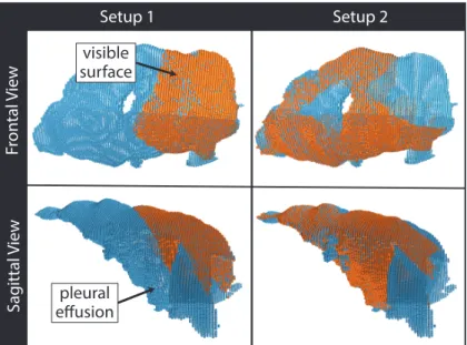
visible surface
pleural effusion
Figure 2.5: The visibility sets found by the motion planner for Setup 1 (left column) and Setup 2 (right column) after 1 hour of computation. The portion of the surface visualized is rendered in
0 10 20 30 40 50 60
Time (m)
0 20 40 60 80 100
Percent Found
Setup 1 Setup 2 Setup 1 / Total Setup 2 / Total
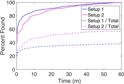
Figure 2.6: The percent of goal points seen by the camera as a function of the motion planner’s exploration time for each setup. Solid lines show the percent of goal points seen by the camera with respect to each setup’s visibility set. Dashed lines represent the percent of goal points seen with respect to the total number of points on the pleural effusion surface.
2.4.2 Motion Planning to View a Specific Goal Point
We next evaluate the motion planner for computing a motion to view a specific goal point using the chip-tip camera. Using≈49,500 goal points on the surface of the pleural effusion, we show in Fig. 2.6 the percentage of the goal points which have been visualized as a function of time. The percentage of points found can be viewed as the probability that the motion planner finds a plan to visualize a goal point if it were sampled uniformly from the set of visible points found by that specific setup (solid lines) or if it were sampled from all points on the interior surface of the pleural effusion (dashed lines). An example of a motion being planned to view a specific goal point can be seen in Fig. 2.7.
2.4.3 Mechanics Solution Seeding
To evaluate the efficacy of seeding the forward kinematics computation with the solution of an already known near-by shape, we repeated the experiments but without the the seeding. Instead, we initialize each shape calculation with the solved solution of only the initial configuration, corresponding to the root node in the tree.
At the end of the hour-long planning time, the motion planner for Setup 1 without the mechanics solution seeding had only planned visualizations for 30% of the total cells inSbounds compared to
Figure 2.7: A motion plan viewed from inside the pleural effusion. Potential points of interest on the interior surface of the pleural effusion are rendered as blue spheres, with the specific goal point rendered in pink. The plan goes from the initial configuration (a), through collision free intermediate configurations (b) and (c), to a configuration in which the tip of the camera tube can view the goal point in (d).
the seeding had only computed motion plans to visualize 38% of the cells compared to the 57% found by the motion planner with the mechanics solution seeding. A stark difference was also found in the number of configurations being added to the tree. For example, from Setup 1, after 1 hour the motion planner without the seeding had only added 2,177 configurations to the tree, while the motion planner with seeding had added 37,855 configurations. For Setup 2, the motion planner without the seeding had added 2,627 configurations, while the motion planner with the seeding had added 36,610 configurations. The≈14times increase in the number of configurations when using the seeding suggests a significantly more expansive motion planning tree capable of viewing more user-specified points of interest.
2.5 Conclusion
the flexible instrument’s entry points into the body, and efficiently handles the expensive computation of CRISP robot kinematics. We also extended the motion planner to estimate the set of points inside a body cavity that can be visually inspected by the camera of a CRISP robot for a given setup.
In future work, we plan to build upon this new motion planner to bring CRISP robots closer to clinical use. We plan to further accelerate the motion planner using sampling heuristics, precom-putation, and parallelization. Additionally, we plan to extend the motion planner to account for uncertainty such as patient motion during the procedure. We also plan to integrate our motion planner with a physical robot prototype and evaluate the performance of the integrated physical system.
CHAPTER 3
Kinematic Design Optimization of a Parallel Surgical Robot to Maximize Anatomical Visibility via Motion Planning
A robot’s kinematic design, i.e., physical parameters fixed prior to the robot’s use that affect a robot’s kinematics, can greatly impact the robot’s ability to perform a task. The quality of a specific kinematic design can vary as the robot’s task and environment changes. In medical robotics, the quality of a robot’s kinematic design is influenced by the specific surgical or interventional procedure it will perform as well as the specific patient anatomy in which it will operate. A suboptimal kinematic design may negatively impact patient outcomes. In this work, we introduce a method to optimize on a patient-specific basis the kinematic design of the CRISP robot [1, 2] to maximize the ability of the robot’s tip camera to view tissues in constrained spaces.
We remind the reader that the CRISP robot is a minimally invasive surgical robot composed of needle-diameter tubes which are inserted into the patient and assembled into a parallel structure (see Fig. 3.1). This assembly is performed using snares, which the tubes use to grip one another.
In addition to snares, other tools can be passed through or placed at the end of the tubes, such as chip-tip cameras, biopsy needles, ablation probes, etc. As the tubes are then manipulated outside the body by robotic manipulators, the shape is changed inside the body to perform the surgical task. Due to the needle-like diameter of the tubes, the CRISP robot has the potential to further reduce invasiveness of minimally invasive surgical procedures such as abdominal, fetal, and neonatal surgery [1, 8]. When a chip-tip camera is mounted at the tip of one of the tubes, the robot can operate as an endoscope, enabling the physician to view the interior surface of an anatomical cavity, such as the abdomen or pleural space (between a lung and the chest wall) [21]. Whereas typical pleural endoscopes have diameters of 7mm and may require an incision as large as 10mm, the CRISP robot requires only needle-size (1-3mm diameter) entry points in the skin.
Figure 3.1: Two images of the CRISP robot, where 2 manipulators adjust the base poses of needle-diameter tubes that are inserted into the body and assembled into a parallel structure. consider as part of the optimization the anatomical entry points of each tube into the patient’s body, which may be constrained by anatomical factors, as well as the snare grasping locations which define the parallel structure of the robot. Appropriately choosing these kinematic design parameters significantly impacts the robot’s ability to view the anatomical sites of interest to the physician (see Fig. 3.2).
Our design optimization approach combines a global numerical optimization method with a motion planner to evaluate the ability of candidate kinematic designs to view the anatomical sites of interest. Specifically, we use the global optimization algorithm Adaptive Simulated Annealing (ASA) [43, 44] to generate candidate designs, which we evaluate using a sampling-based motion planner specifically designed for viewing anatomical sites using the CRISP robot [8]. By evaluating candidate designs with a motion planner, we ensure that a target is considered viewable by the robot only if viewing the target can be achieved by a robot motion that avoids collision with obstacles in the patient anatomy. This guarantees that the evaluation of the design takes into account the motions required by the robot to view the target regions, not just the robot’s theoretical ability to do so in the absence of constrained anatomy.
Design 1
Design 2
Figure 3.2: Different designs can greatly impact the robot’s ability to view the interior surface of a volume via its tip camera. Here we show 2D examples of a robot (blue) and its field of view (yellow) after being occluded by obstacles (red). In Design 1 (top), the robot cannot view much of the interior surface of the volume (the black circle) due to obstacles as it is manipulated through 3 collision-free configurations. However a different design (bottom), which has different entry points into the volume and a different snare grasping location, can view a much larger percentage of the interior surface. improve the robot’s ability to view target regions.
This chapter is based on work originally presented in [11].
3.1 Related Work
Numerical optimization methods have been developed to optimize the design of various medical robots. Another continuum surgical robotic system for which design optimization methods have been developed is the concentric tube robot. Concentric tube robots are similar to the CRISP robot in that they are continuum systems with complex and computationally costly kinematics due to the elastic and torsional interactions between their tubes. The complex kinematics of these devices have motivated unique approaches to their design optimization.
reachable workspace while satisfying anatomical constraints [46]. Ha et al. optimize designs to maximize the concentric tube robot’s elastic stability, a problem which is of particular concern for concentric tube robots [47]. Morimoto et al. take a unique approach to concentric tube robot design by providing a human with an interface to interactively design the tubes of the robot [48]. These works focus on computing goal configurations of the robot for a given design, and as such do not provide a guarantee that there exists a collision freepath, or sequence of configurations, which allows the computed design to achieve a goal configuration.
To accomplish optimization with start to goal path guarantees, Torres et al. integrate a motion planner into the design optimization process, ensuring that valid paths exist to each reachable target for a given design [49], but this method suffers from slow performance. Baykal et al. build upon this method to compute a minimal set of designs that reach multiple targets [50]. Niyaz et al. utilize a motion planner designed to follow surgeon specified tip trajectories [51] to optimize a concentric tube robot’s starting pose [52]. Recently, Baykal et al. provide asymptotic optimality in the design of piecewise cylindrical robots, which includes concentric tube robots, for reaching workspace targets [44]. In this chapter, we build upon this prior work to optimize the kinematic design of the CRISP robot for anatomical visibility, rather than reachability, and show asymptotic optimality under this new optimization metric.
The optimization of surgical port placement, which has parallels to our optimization of needle entry points, has received previous study as well. Liu et al. optimize port placement and needle grasping locations for autonomous suturing [53], but they require as input a discrete set of candidate grasping and port placement locations. Hayashi et al. investigate abdominal port placement by examining the angular relationship between the port location and anatomical sites in the abdomen [54]. They do not, however consider the requirement of more complex motions during the procedure. Feng et al. optimize laparoscopic port placement for robotic assisted surgery by evaluating the robot’s reachable workspace in the patient [55], but do not consider complex motions or obstacle avoidance during the procedure.
optimize over continuous design parameters.
Methods for optimizing the design of serial manipulators has received a large amount of study and include grid-based approaches [62], geometric approaches [63], interval analysis [64], and genetic algorithms [65, 66, 67, 68]. Frequently these methods require simplified kinematic models or restrictive assumptions to achieve computational feasibility, and typically provide no theoretical performance guarantees.
Taylor et al. present a non-linear constrained optimization approach to the simultaneous design of shape and motion for dynamic planar manipulation tasks [69]. Ha et al. explore the relationship between design and motion by leveraging the implicit function theorem to jointly optimize robot joint and motion parameters for manipulators and quadruped robots [70]. These methods, however, do not provide global guarantees and may be subject to local minima.
3.2 Problem Definition
Similar to as in Sec. 2.2, we consider a CRISP robot composed ofn needle-diameter tubes. One of the tubes, the camera tubeρcam, has a chip-tip camera attached to its tip. The rest of the n−1
tubes have snares with which they gripρcamand are denoted ρk wherek is a unique integer label.
3.2.1 Design Space
Let rcam,r1, . . . ,rn−1,∈R3 represent the points at which the tubes of the CRISP robot enter
the patient’s body expressed in a global coordinate system. Let the set of all valid such entry points beR ⊆R3. The entry points into the patient’s body act as remote center of motion (RCM) points,
preventing the tubes from applying lateral load to the patient’s skin during the procedure, and are fixed during the operation of the robot.
The CRISP robot is assembled into a parallel structure where each snare tube ρk grips the
camera tube atsk∈R, the scalar valued arc length alongρcam. The snare grasping locations are
fixed during operation.
We define a kinematic design d of the CRISP robot as a vector describing each tube’s entry point into the body and each snare tube’s grasping location. The open set of all kinematic designs is D ⊆Rn−1×
Figure 3.3: Highlighting the differences between the CRISP robot’s design parameters and configura-tion variables: The CRISP robot’s kinematic design parameters (orange), which must be set before a procedure, include the entry points into the body (rcamor rk) and the snare grasping locations (sk).
The robot’s configuration variables (blue), which can be continuously modified during a procedure, include the tubes’ insertion lengths into the body (`cam or `k) and the tubes’ orientations at the
entry point (Rcamor Rk).
3.2.2 Configuration Space
Once the kinematic design d is fixed and the CRISP robot is assembled inside the patient, the operation of the robot may then be performed by rotating the tubes about their RCM entry points and inserting and withdrawing the tubes from the patient. We define a configuration of the robot as
q= (Rcam, R1, . . . Rn−1, `cam, `1, . . . , `n−1),
whereR∈ SO(3)represents a tube’s rotation at its entry point, and`∈Rrepresents a tube’s insertion length into the patient’s body. The open set of all configurations then becomesQ ⊆ SO(3)n×Rn.
We define a path as a continuous function σ: [0,1]→ Q, where σ(0) =q0, with q0 defined as the
starting configuration of the robot, which may vary for different designs (see Fig. 3.3). 3.2.3 Workspace
We define the robot’s workspace as W ⊆ R3. We define Shape : D × Q × K → W as the
continuous shape function of the robot, whereK is the compact set of points representing the robot’s geometry.
that Shape(d,q,k)∈ O.
A design-configuration pair(d,q)is said to bereachable if there exists a pathσ : [0,1]→ Qwith σ(0) =q0 and σ(1) =q such that for all0≤s≤1,(d, σ(s))is not in collision.
Let View : D × Q × V ×[0,1]→ W be a continuous function defining the view of the robot, whereV represents the set of rays along which the robot can see as determined by the camera’s field of view, and [0,1] is the domain of a distance along the ray. A target regionT ⊆ W is said to be visible from a design-configuration pair if there exists a ray inV that reaches any point in the target region, unoccluded by any obstacle. More formally, a target region T ⊆ W is visible from a design-configuration pair(d,q)if∃v∈ V, r∈[0,1] :View(d,q,v, r)∈T∧ ∀s∈[0, r] :View(d,q,v, s)∈ O./ 3.2.4 Maximizing Viewable Anatomy
Let T = {T1, . . . , Tm} denote the set of m physician-specified target regions that we seek to
view, where each target region denotes an open set of points in the workspace, Ti ⊆ W,∀i∈[m].
We define a target region asviewable under design d if the target region can be viewed from any configuration that can be reached by following a collision-free path. We then define the number of viewable target regions from a givend asΠ(d) :D →[0, m], where
Π(d) :=|TargetRegionsViewable(d)|. (3.1)
TargetRegionsViewable(d) denotes the set of viewable target regions when using kinematic design
d. Our goal then becomes finding an optimal design d∗ such thatΠ(d) is maximized.
3.3 Method
Algorithm 1:CRISP Robot Design Optimization Input:
T: target regions O: obstacles
iinit: initial number of RRT iterations
i∆: RRT iteration increment
Output: d∗: optimal CRISP design maximizing (3.1)
1 i←iinit;Temp←Tempinitial;Πˆcurrent←0;Πˆ∗ ←0
2 dcurrent,q0←random initial design 3 d∗ ←dcurrent
4 whiletime allowsdo
5 d0,q00 ←SampleDesign(dcurrent,Temp, i); 6 targetsViewed←CrispRRT(d0, i,O,q00);
7 Πˆ0 ← |targetsViewed|;
8 if Accept( ˆΠ0,Πˆcurrent,Temp)then
9 dcurrent←d0;
10 Πˆcurrent←Πˆ0;
11 end
12 if Πˆ0 >Πˆ∗ then
13 d∗ ←d0;
14 Πˆ∗←Πˆ0;
15 end
16 i←i+i∆;
17 Temp←UpdateTemperature(Temp);
3.3.1 Exploring Design Space
To explore the CRISP robot’s design space, we leverage the ASA method. ASA is a global optimization algorithm, ensuring it does not become trapped in local optima. ASA works by iteratively improving upon the current best design. It first samples a candidate design some distance from the current design in design space (SampleDesign at line 5 of Alg. 1). It then evaluates the quality of the candidate design (Acceptat line 8 of Alg. 1). If the candidate design is of higher quality than the current design, i.e.,Πˆ0>Πˆcurrent, ASA will accept the candidate design. However,
with some probability Acceptwill accept an inferior design. It is this mechanism that allows the algorithm to avoid local maxima. Both the distance at which it samples and the probability of allowing an inferior design to be accepted depend upon a “temperature" value (Temp in Alg. 1). The temperature is initially set to a large value, but is decreased over time according to a cooling schedule. In this way, early in the optimization process the algorithm is much more likely to explore more distant designs or accept inferior designs, but later in the process converges to a high quality design. Our algorithm keeps track of the best design found through the course of its execution and returns the best design at its conclusion.
3.3.2 Evaluating Candidate Designs
We evaluate the number of target regions viewable by a candidate design d, denotedΠ(d), using a sampling-based motion planner for the CRISP robot [8]. This approach enables our method to estimate the total number of targets which are viewable by a given design, while only considering those configurations reachable by following collision-free paths. The motion planner, CrispRRT, is based on the Rapidly-exploring Random Tree (RRT) algorithm [72] and has the property that the estimate of viewable target regions approaches the correct value as the number of motion planning iterations rises.
Sampling an Initial Configuration The motion planner requires as input a collision-free starting configuration q0 from which to plan motions. In the case of the CRISP robot, q0 depends ond and
is non-trivial to generate.
is known then subsequent configurations can be propagated out using the forces and moments of the previous configuration to seed that guess. This is a key insight behind the CRISP motion planner [8]. There is, however, no previous state with which to seed the initial configurationq0, as all subsequent
configurations are grown from it, and it is unique to a given design. To solve this problem, we require
q0 to be a load free configuration, i.e., one in which the tubes are applying no forces or moments
to each other. This geometrically restricts the shape of the robot to a right triangle without any axial twist applied to the tubes. There are, however, an infinite number of right triangles that pass through the entry points defined by d.
We address this challenge by selecting initial configurations uniformly at random from the set of possible initial configurations which satisfy the design constraints (note that the set of valid initial configurations from which to sample can be defined relatively simply geometrically). The sampled initial configuration is then collision checked against the environment. If it is found to be in collision, it is discarded and another starting configuration is sampled. This process repeats at most itimes (the iteration parameter), or until a collision-free initial configuration is found, whichever comes first. If a collision-free initial configuration is not found, the design is assigned a value of0, and the motion planner immediately returns.
Running the Motion Planner If a valid initial configuration is found, the motion planner is run to determine the design’s set of viewable targets. The motion planner builds a tree in configuration space with collision-free configurations as nodes and collision-free transitions between configurations as edges. During CrispRRT(line 6 of Alg. 1), the motion planner attempts to expand its tree i times, keeping track of the set of all target regions viewable by the robot configurations represented by nodes of the tree.
A sampling-based motion planner which runs for a finite duration may only return an approxi-mation of the viewable set of targets for a given design (as noted in [44] for the case of reachability). To guarantee that the approximations increasingly approach the true value, the number of iterations for which the planner is run is increased byi∆ at each iteration of Alg. 1 (line 16). This allows the
3.4 Analysis
In this section, we prove under mild assumptions the asymptotic optimality of the proposed method, which provides the user a guarantee that the method’s solution will approach a globally optimal kinematic design as more computation time is allowed.
Specifically, we show that the method almost surely converges to a design under which the maximum number of target regions are viewable. This proof builds on ideas from [44] and adapts them to the case of maximizing viewable goal regions. Our approach reduces to showing that the set of optimal designs has non-zero measure and applying results from prior work on design optimization based on the motivating property of ASA. We prove this via open sets, which are either empty or have non-zero measure. In Lemma 1, we show openness of the set of design-configuration pairs for which the configuration is reachable under the design, a useful lemma in its own right. In Lemma 2, we show that the set of design-configuration pairs from which a given target region is visible is also open. We combine these results in Lemma 3 to show that the set of optimal designs is open. Straightforward application of prior work is then sufficient to prove asymptotic optimality in Theorem 1.
3.4.1 Preliminaries
Our proofs use the fact that the inverse images of open and closed sets under continuous functions are themselves open and closed respectively where the inverse image ofA ⊆B under f :C → B (denotedf−1[A]) is the set {c∈C|f(c)∈A}. In the following proofs, we will also frequently refer to the topological projection (or simply projection) from a Cartesian product of topological spaces X×Y to X. The projection of a setZ ⊆X×Y toX is the set{x∈X | ∃y∈Y : (x, y)∈Z}. Two useful properties of projections enable the proofs below. First, the projection of an open set is itself open. Second, ifY is compact, then the projectionX×Y →X of a closed set is itself closed. This latter property is referred to as the Tube Lemma below.
Assumption 1 (Target Regions as Open Sets). Each target region Ti ∈ T, is defined as an open
set.