Kantak_unc_0153D_17398.pdf

ASSET PRICES, LOCAL PROSPECTS AND THE GEOGRAPHY OF HOUSING DYNAMICS

Preetesh Anand Kantak

A dissertation submitted to the faculty at the University of North Carolina at Chapel Hill in partial fulfillment of the requirements for the degree of Doctor of Philosophy in the Department of Finance

at the Kenan-Flagler Business School.

Chapel Hill 2017

©2017

ABSTRACT

Preetesh Anand Kantak: Asset Prices, Local Prospects and the Geography of Housing Dynamics (Under the direction of Riccardo Colacito)

ACKNOWLEDGEMENTS

TABLE OF CONTENTS

LIST OF TABLES . . . viii

LIST OF FIGURES . . . ix

1 INTRODUCTION . . . 1

2 MOTIVATIONAL EVIDENCE . . . 8

2.1 Low Frequency Cross-sectional Evidence . . . 8

2.2 Time-series Evidence . . . 9

3 LITERATURE . . . 11

4 DATA AND VARIABLE CONSTRUCTION . . . 13

4.1 National Data Computation . . . 13

4.2 Price-to-dividend Computation . . . 14

4.3 Validity of Price-to-dividend . . . 16

4.4 Other Independent Variables . . . 19

4.5 Construction of Local Variables . . . 20

5 HOUSING DYNAMICS ANALYSIS . . . 23

5.1 Return Regression . . . 23

5.2 Robustness . . . 25

5.3 Capitalization Rate Regressions . . . 27

6 ECONOMIC FOUNDATIONS . . . 31

6.1 Setup of the Economy . . . 31

6.3 Calibration of the Model . . . 36

6.4 Numerical Results . . . 39

6.5 Further Empirical Implications . . . 42

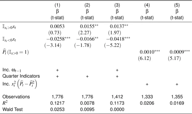
7 IDENTIFICATION OF DURABILITY . . . 44

7.1 Level Regression . . . 45

7.2 Level Regression Robustness . . . 47

7.3 Variance Regression . . . 49

8 CONCLUSION . . . 53

APPENDIX A Gauss-Newton Conversion Algorithm . . . 55

APPENDIX B Dividend and Repurchase Yield . . . 58

APPENDIX C Annual GMM . . . 59

APPENDIX D Extending Annual GMM to Quarterly . . . 60

APPENDIX E Campbell-Shiller Decomposition . . . 63

APPENDIX F Cash Flow Component Extraction . . . 64

APPENDIX G Solving Model’s Equilibrium . . . 66

APPENDIX H Pricing of Aggregate Markets . . . 68

APPENDIX I Simulation Equations . . . 70

APPENDIX J Estimation of Composition Variance . . . 71

LIST OF TABLES

Table 1 Predictive Regressions . . . 10

Table 2 Pre-regression, Conversion Statistics . . . 15

Table 3 GMM and Business-cycle Parameter Summary . . . 18

Table 4 Panel Summary Statistics . . . 22

Table 5 Return Regression Results . . . 24

Table 6 Return Regression Robustness Results . . . 26

Table 7 Capitalization Rate Regressions . . . 29

Table 8 Model Calibration . . . 36

Table 9 Aggregate Calibration Regressions . . . 38

Table 10 Identification Regressions . . . 46

Table 11 Identification Robustness Regressions . . . 48

LIST OF FIGURES

1

INTRODUCTION

This paper shows that the cross-section and time-series of long-run industry growth prospects is a key factor in explaining the geographic differences in home prices. I use a market based mea-sure of growth prospect to quantify theuniquerelationship between prospects and housing re-turns. I document that a decline in local growth prospects is associated with a decrease in the ex-pected housing risk premia and an increase in the price-to-rent ratio. I attribute these finding to the hedging characteristics of housing assets and replicate them in a consumption based asset pric-ing model in which (1) investors care about the temporal distribution of uncertainty, (2) consump-tion of non-housing goods and housing services are exposed to time-varying, long-run growth prospects, and (3) housing services provide a hedge against negative news about expected long-run growth. In addition, I show strong empirical evidence of these hedging characteristics in the geographic cross-section of consumption data.

Real estate is a significant portion of aggregate wealth in the United States. The total value of household real estate is approximately$25 trillion, which is greater than the almost$23 tril-lion households have in corporate equity. Even after netting this gross figure by the$9.3 trillion in household mortgage liabilities, the portion of wealth concentrated in real estate is staggering. U.S. GDP figures show a similar picture; expenditures on shelter account for almost 20% of the nation’s annual consumption (Federal Reserve Q4 2015 statistical release). These aggregate fig-ures, however, belie the inherent geographic differences in real estate wealth across the country (see Gyourko, Mayer and Sinai (2013)).

Bartels-man, Haltiwanger and Scarpetta (2013) for recent work). It follows from this evidence that growth prospects of the local industry mix should be reflected in geographic differences in economic growth and price dynamics of local (segmented) asset classes. Housing is the segmented asset I use for my empirical analysis; its value is intimately tied to its location. For example, the struc-tural transformation of the United States from a largely manufacturing to service based economy has played out differently over long-horizons between the industrial Midwest and the globally in-tegrated, finance and technology hubs on the coasts. My analysis shows that these differing eco-nomic fundamentals have had important implications for local housing returns. This paper seeks to understand how house prices move in the context of its role as both alocal consumption asset (i.e. provides access tolocal growth opportunities) and the primary store of wealth for the median household. As such, my findings have important implications for, inter alia, the transmission of monetary and fiscal policy to inclusive and broad sectoral economic growth, and long-run income inequality.

be different from those that do not. These two assumptions are similar to those made by Bekaert, Harvey, Lundblad and Siegel (2007). In their study they compute measures of country-level growth opportunities by weighting industry price-to-earnings (PE) ratios to understand the cross-section of emerging market returns. In the same spirit, I weight industry PDs by local employment share to understand the cross-section of MSA-level asset returns.

I run predictive regressions to show that my measure of local prospects explain a substantial portion of variability in the cross-section and time-series of excess housing returns. I find that a one standard deviation increase in my proxy of local prospects leads to a statistically significant 120bp increase in annual excess housing returns. In addition, I decompose my measure of local prospects into a common (all-MSA or global) and orthogonal (local) component. A one standard deviation increase in the global, and local component leads to an statistically and economically significant 150bp and 35bp increase in annual excess returns, respectively. Surprisingly, although my industry-level measures are taken from the aggregate markets, their impact is geographically heterogenous due to differences in MSA-level employment composition. These return predictabil-ity findings are robust to various business cycle controls from the literature (see, e.g., Abraham and Hendershott (1994); Favilukis, Kohn, Ludvigson and Van Neiuwerburgh (2013); and Tuzel and Zhang (2016)).

local prospects lowers the log price-to-rent by more than 500bps. The negative coefficient implies that the expected return dominates the expected rent channel.

These risk based results stand in contrast to the findings of traditional predictive regressions. In the equity market better prospects, which are typically associated with high PD-ratios, usually imply less risk and therefore lower expected excess returns going forward (see Campbell and Shiller (1988); Cochrane (2008); Lewellen (2004)). The key difference between housing and other consumption assets, however, is the relative durability of the services that it provides. Housing is anextremely durable asset: when local prospects are good they strongly influence plans to build infrastructure and locate close to suppliers of capital and labor (i.e. agglomeration economies). Once in place these pieces are both permanent in nature and geographically specific. For exam-ple, New York City and San Francisco will likely continue to be centers of finance and technology regardless of higher frequency economic fluctuations. Thus, in the context of risk to housing, this permanence acts as a hedge against negative shocks to long-run local growth prospects. Urban economists have argued that the durability ofphysical structuresis key to understanding many multi-decade phenomena in urban and labor economics (see Glaeser and Gyourko (2005) and Notowidigdo (2013)). My argument is similar regarding the durability of the location specific ser-viceshousing provides.

First, recursive preferences are required to price persistent dynamics, such as those of my measure of local prospects (see inter alia Bansal and Yaron (2004), Colacito and Croce (2011, 2013)). Second, the persistence of my state variable contains important information in that its fluctuations embed long-horizon implications. This feature has immediate intuitive appeal when it comes to the pricing of long-lived assets such as housing. The asymmetric exposure to prospects reflects the hedging quality of housing services; once they are “built” they are difficult to take away. In addition, both non-housing and housing endowments have short-run i.i.d. shocks. These shocks reflect higher frequency business-cycle or MSA-level idiosyncratic shocks.

This simple setup means that the endowment of housing is exposed to two sources of risk when growth prospects are high (short- and long-run), but only one when growth prospects are low (short-run). Theexpected risk to housing thus becomes a function of the conditional probabil-ity of being in a high expected growth state tomorrow. In addition, as growth prospects are highly persistent, this probability is increasing in the expected growth rate of consumption, giving the re-turn profile characteristics of a regime switching model. I then replicate my empirical results by simulating 375 MSAs over 40yrs and conduct both the predictive excess return and contempora-neous PS-ratio regressions on generated data. My average coefficients are close to their empirical counterparts. A one standard deviation higher growth prospect leads to a 110bp increase in ex-pected return. The model illustrates how durability of housing services with respect to long-run growth prospects generates time varying volatility in the ratio of housing services versus non-housing consumption (henceforth relative consumption), which has immediate implications for return and pricing dynamics.

in prospects leads to a much smaller rise in relative consumption. This suggests that the local households raise consumption of housing services in lock step with non-housing consumption dur-ing times of good long-run economic prospects, but do not drop them as much as non-housdur-ing consumption during bad times. This evidence is not present in renter consumption data; I find that a one standard deviation fall and rise in long-run growth prospects lead to an equally large rise andfall of relative consumption. This suggests that “sticky” contracting issues are not the primary driver of my results. I also confirm the profile of time varying volatility in the data. The variance of relative consumption increases by more than 700bps from the low to high variance regime. Given the high persistence of the underlying economic state variable, this increase in variance has a long-horizon impact on housing consumption decisions. This verifies the model’s primary risk channel.

Figure 1: Industr y Concentr ation and Cross-sectional Evidence P anel 1A captures the distr ib ution of Herfindahl-Hirschman Indices (HHI) across 61 industr ies an d 375 MSAs on December 31st, 2011. Em-yment share for each industr y i and MSA a is defined as

si,a

=

E

m

pi,

a

/∑

375 k=

1

E

m

pi,

k . HHI for industr y i is defined as the sum of squared shares all 375 MSAs . P anel 1B projects the a v er age MSA-le v el emplo yment share w eighted PD-r a tios from 1991-2000 for the 100 most populated . P anel 1C projects MSA-le v el real per-capita GDP from 2001-2010. Data is from The Bureau of Economic Analysis (BEA). P anel 1D projects v el a v er age housing e xcess pr ice appreciation from 2001-2010. Data is from the FH F A . The colors (g reen-y ello w-red scale) correspond to fiv e siz ed b uc k ets rank ed from the lo w est to highest 20% of each v ar iab le . A: 2011 Herfindahl-Hirschman Indices

IT, Computer Design Auto, Machine Manuf. Investments, Financial Vehicles

Motion Pictures Oil and Gas Extraction

2

MOTIVATIONAL EVIDENCE

I use the aggregate industry PD ratio to obtain measures of industry-specific growth oppor-tunities for two reasons. First, I would like my measure to reflect heterogeneity in prospects only because of geographic differences in industry clustering. Second, given its durable nature and role as both a consumption good and component of wealth, housing is exposed in a fundamentally different way than stocks, both in magnitude and direction, to long-run sources of economic risk. It’s important that my measure captures this difference. In this section, I’ll show evidence that my measure of long-run growth prospects satisfies both requirements.

2.1 Low Frequency Cross-sectional Evidence

Location specific measures of prospects (e.g., price-to-rent) are 1) limited in availability and

quality, and 2) confounded by geographic-specific information orthogonal to long-run growth prospects (e.g., weather or regulatory factors). To better motivate the specific type of geographic risk in

lowest excess price appreciation, respectively. The intra-decade spatial correlation between these returns and the local average PD from 1991-2000 is more than 60% and significant at a 5% level. There seems to be strong association between geographic heterogeneity in output and housing returns and differences in industry prospects and employment composition.

2.2 Time-series Evidence

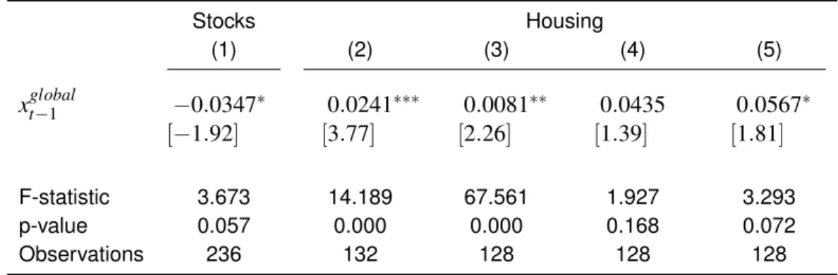
Table (1) highlights the difference between housing and stocks in their exposure to long-run growth prospects using times-series regressions on aggregate indices on a quarterly basis. Col-umn (1) is the classic Campbell and Shiller (1987) result using data from 1953-2014; the excess return of the stock market is regressed onto my economic state variable, the lagged market PD ratio (xglobal_t−1 ). The state variable predicts excess returns on housing with a statistically significant negativecoefficient. This results fits the intuition that high PD-ratios reflect a conditionally better economic environment, signifying lower economic risk. The marginal agent thus demands a lower risk premia in such circumstances. Cochrane (1994), Bansal and Yaron (2004), Lettau and Ludvig-son (2005) and others have explored the underlying economic drivers of this result. In column (2) I regress housing excess returns onto my state variable. Aggregate economic prospects predict aggregate housing returns with apositiveand statistically significant coefficient.

Table 1:Predictive Regressions

This table reports results from predictive regressions of excess returns for the stock and hous-ing markets onto the lagged market price-to-dividend, my state variable of interest (x_tglobal₋₁ ). The re-gressions are on quarterly data. Following the methodology of Boudoukh, Michaely, Richardson and Roberts (2007), my measure of dividend includes share repurchases. Model (1) is the classic Camp-bell and Shiller (1987) result using data from 1953-today. Model (2) regresses housing excess returns onto my state variable. Housing returns are computed from the Shiller repeat sales index available online at http://www.econ.yale.edu/ shiller/data.htm. A national estimate of rent is then added to obtain a proper return measure (see http://www.lincolninst.edu/). The 3m T-bill rate is then subtracted from this measure. Repeat sales indices are highly persistent and demonstrate seasonality by construction; in model (3) I include the excess return quarter and annual lag as regressors. Columns (4) and (5) are the result from regressing excess returns on the general REIT universe and multi-family home REITS, respectively, onto the lagged market price-to-dividend ratio (x_t−global₁ ). The REIT indices are from the CRSP Ziman real estate total return data series. The sample size falls from the Campbell-Shiller to housing return regressions because rent and REIT data is only available after the 1980s.

Stocks Housing

(1) (2) (3) (4) (5)

x_tglobal₋₁ −0.0347∗ 0.0241∗∗∗ 0.0081∗∗ 0.0435 0.0567∗

[−1.92] [3.77] [2.26] [1.39] [1.81]

F-statistic 3.673 14.189 67.561 1.927 3.293

p-value 0.057 0.000 0.000 0.168 0.072

Observations 236 132 128 128 128

3

LITERATURE

This paper extends work done in the long-run risk asset pricing literature. Bansal and Yaron (2004) show that highly persistent, low-frequency dynamics in consumption and recursive pref-erences (collectively known as long-run risk) are important in explaining the equity risk premia puzzle. Colacito and Croce (2011, 2013) utilize these same dynamics and preferences to better understand key international asset pricing dynamics such as the currency risk premia. My empir-ical specification is similar to that of Gomes, Kogan, and Yogo (2009) and Eraker, Shaliastovich and Wang (2016) in that I attribute heterogeneity in asset price dynamics to heterogeneity in long-run dynamics of different firms or industries.

This paper also relates to a strand of the macroeconomic literature that links housing to asset prices and consumption behavior. Piazzesi, Schneider and Tuzel (2007) show that non-separable composition risk between housing and non-housing consumption can explain a significant por-tion of the equity premium puzzle. Lustig and Van Nieuwerburgh (2005, 2009) find connecpor-tions between housing collateral, consumption and asset prices. My objective is somewhat more funda-mental in that I seek to understand how persistent local growth prospects impact the risk premia of home prices because of their inherent geographic heterogeneity rather than vice versa.

My geography-centric approach is largely related to work done in urban economics. Begin-ning with Rosen (1979) and Roback (1982), urban economists have used spatial general equilib-rium models to understand geographic heterogeneity in home prices and productivity.1 In terms of higher frequency home fluctuations, Glaeser, Gyourko, Morales and Nathanson (2014), show that a spatial equilibrium model with durable housing and lagged investment, explain certain housing return “puzzles.” Their model and calibration, however, largely ignores the importance of

time-1_{See Glaeser and Gyourko (2005); Glaeser, Gyourko, and Sacks (2005); Van Nieuwerburgh and Weill (2010); Kline}

varying expectations and risk aversion in prices. Hizmo (2015) blends a spatial equilibrium with a real business cycle model to estimate the housing risk-premia in different cities. While risk aver-sion plays an important role, agents ignore conditional dynamics of expectations when making decisions on how much housing services to consume.

4

DATA AND VARIABLE CONSTRUCTION

In this section I present the sources of my data and the methods used to validate my estimate of long-run prospects. I first introduce my aggregate measure of industry output. I then extract my industry-level measure of prospects and show that it strongly predicts the industrial cross-section of real per-capita output. I weight this measure of prospects using MSA-level employment compo-sition data to obtain a local measure of long-term growth prospects. My methodology follows that of Bekaert, Harvey, Lundblad and Siegel (2007). In keeping with an established literature, I occa-sionally refer to these prospects as long-run risk (see Bansal, Kiku and Yaron (2012) and Colacito and Croce (2011) for references).

4.1 National Data Computation

My measure of aggregate industry output is from The Bureau of Economic Analysis (BEA) -US-wide (aggregate) value-added and employment data for approximately 60 broad industries running from 1947 to today. The data is primarily at the 3 digit NAICS (North American Industry Classification System) or 2 digit SIC (Standard Industry Classification) level. The NAICS data is available from 1977 to today and SIC data from 1947 to 1997. I convert this data into a single clas-sification system to properly identify the strengths of my measure of long-run industry prospects (see section (4.3)). In order to best capture the more contemporary trends in GDP and employ-ment away from manufacturing towards information technology and services, I convert the older (SIC) to the newer (NAICS) system.

output and employment (see APPENDIX A for details on my conversion algorithm). Table (2A) provides the summary statistics of the NAICS to SIC conversion weights. I now have an estimate for value-added GDP and employment from 1947-2012 for a single industry classification. The value-added GDP data is deflated by industry specific deflators. Aper-capitameasure is com-puted by dividing each industry’s value-added GDP by its employment figure.

4.2 Price-to-dividend Computation

The regressions presented in section (5) require an estimate of the price-dividend (PD) ratios for the same 61 NAICS industries for which I now have value-added GDP. I compute PD ratios us-ing data from the Center of Research in Security Prices (CRSP).2Following Boudoukh, Michaely, Richardson and Roberts (2007), I also include share buybacks in my measure of dividend (see APPENDIX B for details). Including this payout is critical in comparing industry prospects due to heterogeneity in repurchases yields (RPt) across industries. This is similar to what is done by Gomes, Kogan and Yogo (2009), although on a more disaggregate industry basis.

For my analysis, I require both annual and quarterly PD ratios. Given its monthly frequency, the dividends from CRSP are simply summed on both basis. For example, if there areN compa-nies within industry i, dividends for annual or quarterly t are summed if they are in(t−m,t), where

mis 11 and 2 for each frequency, respectively. The dividend yield is thus

DP_ti= ∑ t

k=t−m∑Nj=1 ShrOutj,k

Div_j,k

∑Nj=1 ShrOutj,t

Px_j,t .

For CRSP data, quarterly seasonality is minimal so this simple change in index is sufficient to obtain accurate yields at both frequencies. This is not the case with repurchases, where taxes and regulatory considerations affect timing of company actions. For my quarterly projections, I thus evenly divide a given year-industry’s annual repurchases over the four quarters. My PD ratio measure is the inverse of dividend and repurchase yield,1/(DPt+RPt).

2_{See van Binsbergen and Koijen (2010) for references. CRSP distribution codes are restricted to all cash ordinary}

Table 2:Pre-regression, Conversion Statistics

I use the crosswalk between 3-digit SIC and 6-digit NAICS codes from the Bureau of Labor Statis-tics (BLS) to convert SIC to NAICS GDP. Indicators are given to each correspondence and then rolled-up to the BEA-available primarily 3-digit SIC level. The first line of Panel A provides summary statistics of how many NAICS industries each SIC account converts. The BEA SIC and NAICS GDP and em-ployment data also have common years from 1977 to 1997. As detailed in APPENDIX A, using this 1-to-N correspondence and the common years, I use a iterative algorithm to estimate SIC-to-NAICS conversion weights for the years NAICS data is not available. The balance of Panel A provides pro-vides the summary statistics of these estimated weights over various subsamples. Panel B are the summary statistics of my price-to-dividend ratio from 1947-2011. Cash dividend (distribution codes 1xxx and 2xx2/2) yields are estimated from the full CRSP database - I sum the dividends paid by a given industry (forPD_tind) or the “market” (forPDmkt_t ) over either the quarter or year and then divide by the total market capitalization on the last month of said period. Intra-period dividends are reinvested at the risk-free rate. Repurchase yields are computed from COMPUSTAT data. I compute repurchases following Boudoukh, Michaely, Richardson and Roberts (2007). In order to remain internally consis-tent, I remove each industry’s price and dividend information in the measure of its market PD-ratio. PD-ratios are the inverse of the cash dividend plus repurchase yields.

A:SIC-to-NAICS Statistics

N Mean p25 p50 p75 max/min

SIC-to-NAICS Count 60 4.13 2.00 3.50 5.00 19.00

1977-1997 weights:

Employment 247 0.24 0.02 0.12 0.35 0.00

Value-added GDP 247 0.24 0.02 0.12 0.33 0.00

1977-only weights:

Employment 247 0.24 0.02 0.12 0.33 0.00

Value-added GDP 247 0.24 0.02 0.11 0.32 0.00

1997-only weights:

Employment 247 0.24 0.02 0.11 0.35 0.00

Value-added GDP 247 0.24 0.01 0.11 0.32 0.00

B:Price-to-Dividend Statistics

Composition PD statistics

n(max) n(min) mean sd skewness kurtosis

log(PDmkt_t ): 8806 721 4.62 0.30 -0.11 2.49

log(PDind_t ):

Summary statistics of my PD measure are presented in table (2B). As can be seen, over my sample there is sharp increase in the number of companies at both the market and industry-specific level over time. For example, during the early years almost 25% of industries have 3 or less char-acteristic firms in my PD-ratio estimate. The sharpest increase in firm composition comes be-tween the years 1960 to 1975, during which the AMEX and NASDAQ were introduced to CRSP.

4.3 Validity of Price-to-dividend

The premise of my analysis is that industry PD-ratios embed realistic expectations of an indus-try’s future cash flow and riskiness. In this section, I use a predictive regression approach, initially used in work by Harvey (1988), to show that this is in fact the case. More recently, Bansal, Kiku and Yaron (2012) and Colacito and Croce (2011, 2013) use a similar approach in the long-run risk context. Specifically, I show that the past industry and market PD-ratios computed in section (4.2) project next period industry value-added GDP growth computed in section (4.1). Assuming that expectations of GDP growth are, on average, correct, this intuition is captured in a simple regres-sion for industryi,

∆yi,t+1=βpdi,t+εi,t+1,

where lower case letters signify the log of each variable.

(2004)). I thus include the annualized 3m treasury bill rate in the projection. Finally, these long-run expectations of output and riskiness tend to be extremely persistence. I capture this persistence as an AR(1) process. The motivating idea is that investment decisions, especially those of large scale, entail projecting economic growth substantially in the future and are usually made ignoring higher frequency, “temporary” economic (e.g., business) cycles. For example, Croce (2014) and Colacito, Croce, Ho and Howard (2013) use persistent AR(1) process in TFP growth to capture previously unexplained production and asset price puzzles.

My primary system of equations for any industryiis thus,

pdi,t =γipd−i,t+ηi,t, (1)

∆yi,t+1=βipd−i,t+αiηi,t+δirtf+ei,t+1,

x_i,t =βipd−i,t+αiηi,t+δirtf =ρixi,t−1+εi,t.

The first equation of system (1) captures the decomposition of the industry PD-ratio onto its market (captured byγ) and industry-specific (ηt) components. In order to remain internally consis-tent, I remove each industry’s price and dividend information in the measure of its market PD-ratio (i.e. pd_−i,t). The second equation of system (1) is the projection or predictive regression. If the PD-ratio embed information about long-run expectations of industry cash flows, a negativeβand αimplies that agents ascribe “safety” to the industry’s cash flows. Intuitively, one would assume non-durable industries, such as food-manufacturing, would exhibit negativeβs, whereas tech-nology related industries, such as computer-manufacturing, would exhibit positiveαs. The third equation of system (1) parameterizes the persistence of these expectations.

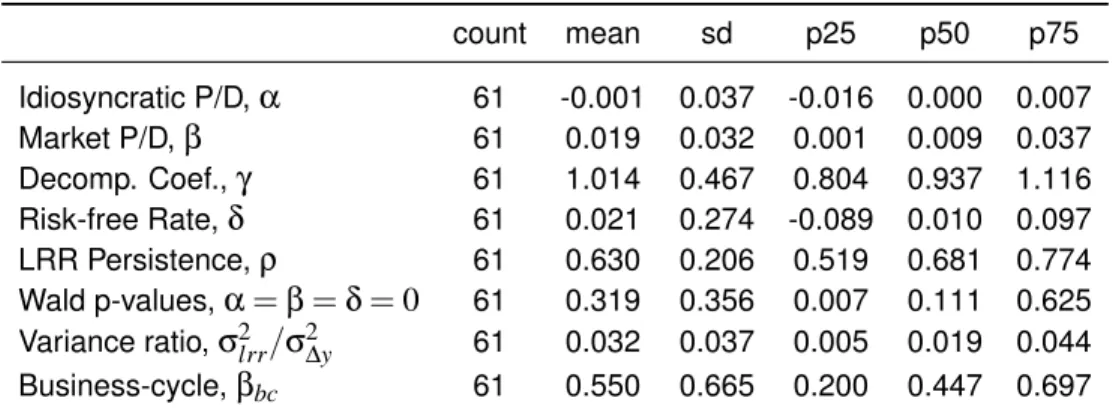
Table 3:GMM and Business-cycle Parameter Summary

This table reports the GMM parameter statistics from section (4.3). Separate GMM regressions are run for each of my 61 NAICS industries from 1948 to 2012 with either annual (Panel A) or quarterly (Panel B) data. This allows me to jointly estimate my projection equations. The moment conditions for the quarterly GMM require minor modifications due to the mixed-frequency data. Those details are in APPENDIX D. In addition, I provide results of a Wald statistic that test whether the main projection coefficients are jointly different than zero, and estimates of the business-cycle beta from equation (2). Results are given at the 25th, 50th, and 75th percentiles.

A:Annual Parameters and Statistics

count mean sd p25 p50 p75

Idiosyncratic P/D,α 61 -0.001 0.037 -0.016 0.000 0.007

Market P/D,β 61 0.019 0.032 0.001 0.009 0.037

Decomp. Coef.,γ 61 1.014 0.467 0.804 0.937 1.116

Risk-free Rate,δ 61 0.021 0.274 -0.089 0.010 0.097

LRR Persistence,ρ 61 0.630 0.206 0.519 0.681 0.774

Wald p-values,α=β=δ=0 61 0.319 0.356 0.007 0.111 0.625

Variance ratio,σ2_lrr/σ2_∆y 61 0.032 0.037 0.005 0.019 0.044

Business-cycle,βbc 61 0.550 0.665 0.200 0.447 0.697

B:Quarterly Parameters and Statistics

count mean sd p25 p50 p75

Croce (2011) and Bansal, Kiku, Yaron (2012). In addition, high and lowβindustries are largely composed of durables (e.g., autos) and non-durables (e.g., food), respectively. In addition, the null for the Wald testα= β=δ=0is rejected for nearly 50% of the industries at a 5% level, pro-viding evidence that past PD-ratio provide insight into future industry output. Much of the data I use can also be extracted at an quarterly frequency. Table (3B) shows that higher frequency data yields even stronger evidence of this predictive relationship (see APPENDIX D for methodology). My result validate the usefulness of industry price-to-dividend as a measure of prospects. For the specifications where an industry’s PD-ratio is split into its market and industry components, I sim-ply useγipd−i,t andηi,tfrom system (1), respectively. Given the nomenclature used in system (1), henceforth pdi,t,γipd−i,t,ηi,t will be referred to asxi,t,xglobal_i,t andxlocal_i,t , respectively.

4.4 Other Independent Variables

From the Campbell-Shiller decomposition (see APPENDIX E for derivation), one can see that the PD-ratio is a convolution of expected dividend growth and expected returns. Given the eco-nomic story I developed in section (2), it would seem that the cash flow rather than the return com-ponent of the PD-ratio would be the primary driver of real estate dynamic. I exploit the standard ICAPM risk and return relationship to derive a measure of long-run industry prospect that seeks to extract only the cash-flow portion from the industry price-to-dividend ratios (see APPENDIX F for details). I refer to the alternative measure of industry prospect asx_tc f.

In addition, it is important that I isolate the impact of long-run industry prospects on housing returns from those of higher frequency (henceforth business cycle) dynamics. Previous literature has shown that housing returns are strongly effected by cycles of higher frequency (see Davis and Heathcote (2005) for literature overview). For my analysis in section (5), I use three measures of business cycle risks that are motivated in Tuzel and Zhang (2016). Two utilize the beta estimate, βbc, from regressing my annual industry value-added GDP onto annual national GDP growth, i.e.

∆y_ti=βbc 4

∑

q=1

Details of the construction of these three measure are provided in the next section. The sum-mary statistics from the cross-section ofβs from this regression are also provided in tables (3A) and (3B).

In summary, given consistent parameter estimates at two frequencies, I am comfortable con-structing point estimates of the long-run industry prospects,x_t, for all 61 aggregate NAICS indus-tries. In addition, following Tuzel and Zhang, I estimate business cycle variables for these same industries. The next step is to “localize” these aggregate measures.

4.5 Construction of Local Variables

I weight each industry variable estimated at the aggregate level with the industry’s employ-ment share at the local MSA level and then sum to obtain my local variable. In the urban and labor economics literature this methodology is called the Bartik (1991) procedure and is used to gener-ate measures of local “demand” from aggreggener-ate market measures (see Bound and Holzer (2000), Autor and Duggan (2002) and Luttmer (2005) for applications). In the financial context, Bekaert, Harvey, Lundblad and Siegel (2007), Davidoff (2015), and Tuzel and Zhang (2016) have motivated similar approaches in their analysis. I use the procedure to connect aggregate industry prospects to growth prospects of local economies.

For example, my MSA-level long-run prospect measure for any period,t, and MSA,msa, is

xmsa,t = I

∑

i=1

si,msa,txi,t, (3)

wheres_i,msa,t is the fraction or share of total employment of industryiinmsaat timet. My source of MSA-level employment data is the BLS quarterly census of employment and wages (QCEW) data. Applying the Bartik procedure, even dynamics that vary across only industry (e.g.,βbc) will now vary in both space and time due to changes in employment composition - e.g.,βbcbecomes βbc_msa,t.

dele-tion of counties, it is important that my employment shares are consistent with my main dependent variable, the MSA-level FHFA excess housing returns. I thus download county level employment data and aggregate up to the MSA using the most recent BLS county-to-MSA crosswalk. My re-gressions are also supplemented with four measure of business-cycle variation for each MSA. The first is simplyβbc_msa,t. The second is the aggregate GDP growth,∆yt. The third is the expectation of industry GDP growth given its beta exposure to the GDP shock, i.e. βbc_msa,t−1×∆yt. Finally, em-ployment growth itself may be an important predictor of real estate returns. The fourth addition is thus the MSA Bartik-localized employment growth,∆empmsa,t.

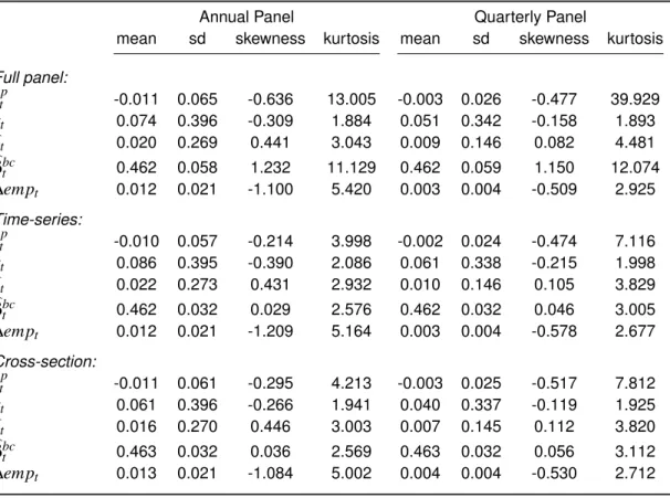
Table 4:Panel Summary Statistics

This table reports summary statistics of my estimated MSA-level dependent variable and re-gressors using the annual and quarterly frequency data. I localize these rere-gressors by following the Bartik (1991) procedure - each industry variable I estimate at the aggregate level is interacted with the MSA-level employment share and then summed at a MSA-level. Summary statistics are also given on samples collapsed either cross-sectionally (375 MSAs) or by time-series (35yrs).rtpis the excess price

appreciation estimated by the MSA-level FHFA repeat sales indices._bxt is my industry specific measure

of long-run risk - the demeaned industry pd-ratios,bεt is the residual from system (1),β

bc_{is the}

busi-ness cycle beta computed from equation (2) and∆empt is the employment share weighted average

aggregate industry employment growth.

Annual Panel Quarterly Panel

mean sd skewness kurtosis mean sd skewness kurtosis

Full panel:

rtp -0.011 0.065 -0.636 13.005 -0.003 0.026 -0.477 39.929 xt 0.074 0.396 -0.309 1.884 0.051 0.342 -0.158 1.893

bεt 0.020 0.269 0.441 3.043 0.009 0.146 0.082 4.481 b

βbct 0.462 0.058 1.232 11.129 0.462 0.059 1.150 12.074 ∆empt 0.012 0.021 -1.100 5.420 0.003 0.004 -0.509 2.925 Time-series:

rtp -0.010 0.057 -0.214 3.998 -0.002 0.024 -0.474 7.116 xt 0.086 0.395 -0.390 2.086 0.061 0.338 -0.215 1.998

bεt 0.022 0.273 0.431 2.932 0.010 0.146 0.105 3.829 b

βbct 0.462 0.032 0.029 2.576 0.462 0.032 0.046 3.005 ∆empt 0.012 0.021 -1.209 5.164 0.003 0.004 -0.578 2.677 Cross-section:

rtp -0.011 0.061 -0.295 4.213 -0.003 0.025 -0.517 7.812 xt 0.061 0.396 -0.266 1.941 0.040 0.337 -0.119 1.925

bεt 0.016 0.270 0.446 3.003 0.007 0.145 0.112 3.820 b

5

HOUSING DYNAMICS ANALYSIS

5.1 Return Regression

My full regression specification is,

r_msap _,t=b_xx_msa,t−1+Time FE+MSA FE+Controls+εmsa,t. (4)

My business cycle control variables from section (4) areβbc_msa,t−1, which captures the expo-sure orβof the local industry mix to changes in aggregate gdp; the interaction of thisβand ag-gregate GDP growth,βbc_msa,t−1×∆yt; and the five year average local industry employment growth, ∆empmsa,t−1. Given that I have time fixed-effects, variation in credit supply and contemporaneous shocks to GDP, will not drive my results (see Favilukis, Kohn, Ludvigson and Van Nieuwerburgh (2013) for discussion). This is especially important due to the credit boom-bust cycle from 2006-2009. In addition, I include the lagged MSA return premia,r_msap _,t−1, as a control due to the highly degree of autocorrelation in return measures computed from repeat-sale indices (see Ghysels, Plazzi, Torous, Valkanov (2012)).

My primary coefficient of interest isb_x. In section (2) I showed that a geographic concentration of high PD-ratio industries today seems to imply greater excess price appreciation going forward.

x_msa,t is a employment weighted average of the PD-ratios of industries within a particular MSA. I would thus expect thatb_x is positive and significant. I conduct this analysis for annualx_msa,t; the results are presented in table (5). All variables are standardized, representing the marginal effect from a one standard deviation move in the regressor.

Table 5:Return Regression Results

This table reports the regression results of equation (4) given annual data. I cluster standard er-rors along MSA. The repeat-sales method used to computed the FHFA price indices has a high degree of autocorrelation in returns by construction. I thus include the lagged MSA return premia,r_t−p ₁, as a control. Model (1) is the regression on the full sample. Model (2) splits my measure of long-run local growth prospects into its market-wide (global) and MSA-specific (local) components. Model (3) adds the Tuzel and Zhang (2016) motivated business cycle variables. Model (4) adds the estimated local expected employment growth. Model (5) uses the MSA-level rental data from Campbell, Davis, Gallin and Martin (2009) for a cross section of 23 MSAs from 1975-2007. As this regerssion limits the time series and cross-section, I do not include MSA and time fixed effects, but rather cluster along both di-mensions. I also add the credit supply variable from Favilukis, Kohn, Ludvigson and Van Nieuwerburgh (2013). *, **, and *** denote significance at the 10%, 5%, and 1% levels.

(1) (2) (3) (4) (5)

β [t-stat]

β [t-stat]

β [t-stat]

β [t-stat]

β [t-stat]

xmsa,t−1 0.0126∗∗∗ 0.0120∗∗

[6.29] [2.32]

b

xglobal_msa,t−1 0.0155∗∗∗ 0.0141∗∗∗ 0.0175∗∗∗

[10.42] [8.43] [8.73]

b

xlocal_msa,t−1 0.0036∗∗ 0.0038∗∗ 0.0036∗∗

[2.21] [2.34] [2.24]

Inc.r_t−p ₁ + + + + +

Inc._bεt + + + + +

BC Controls + + +

Inc.∆empt−1 + +

FKLVcs +

Observations 10,003 10,003 10,003 10,003 586

R2 0.5078 0.5084 0.5089 0.5100 0.5349

Wald Test 0.0000 0.0733 0.0001

rejected as seen by the Wald Test p-value. Column (3) and (4) add the business cycle variables. While the business cycle regressors contribute to explaining the variation in excess returns (see Wald tests p-values), they explain substantially less than the long-run prospect derived variable (xmsa,t). Finally, our measure of price appreciation is not a proper total return measure as it does not include rent. Campbell, Davis, Gallin and Martin (2009) derive a measure of rent for a cross section of 23 MSAs from 1975-2007 using Census data. I add rent to the price appreciation and limit the regressions to these years and MSAs. The results are in column (5). As the cross-section and time series are now limited, I no longer include MSA and time fixed effects, but cluster along both dimensions following Petersen (2009). All results point to the same conclusion - the better the conditional prospects the higher the expected returns next period.

5.2 Robustness

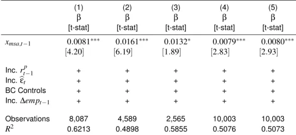
Table 6:Return Regression Robustness Results

This table reports robustness results for the regressions presented in table (5). Details on standard errors and controls are identical to those applied in that table. Model (1) uses data from 1990-2011, which removes employment share estimates using converted employment data. Suppression of certain count-year employment data from the QCEW may be a problem in estimating my coefficients. I specify an indicator where each county-msa employment data is not disclosed. I then compute the percentage of county-industries within an MSA with suppressed data. Model (2) restricts the sample over which I run regression (4) to only those MSA-yearss where< 10%of its county-industries are suppressed. Model (3) restricts the sample to MSA-level populations of>680,000, which represents the top 25% of MSA size. Model (4)- (5) tweaks my employment share measure to include lagged employment growth to varying degrees; the tilt parameter,λ, is 1 and 5 for (5) and (6), respectively (see section (5.2) for details). *, **, and *** denote significance at the 10%, 5%, and 1% levels.

(1) (2) (3) (4) (5)

β [t-stat]

β [t-stat]

β [t-stat]

β [t-stat]

β [t-stat]

xmsa,t−1 0.0081∗∗∗ 0.0161∗∗∗ 0.0132∗ 0.0079∗∗∗ 0.0080∗∗∗

[4.20] [6.19] [1.89] [2.83] [2.93]

Inc. r_t−p ₁ + + + + +

Inc.bεt + + + + +

BC Controls + + + + +

Inc. ∆empt−1 + + + + +

Observations 8,087 4,589 2,565 10,003 10,003

R2 0.6213 0.4898 0.5855 0.5076 0.5073

of>680,000, which is the 25th percentile of MSA size across my panel, the coefficient of interest shows similar economic and statistical significance.

em-ployment in that industry will grow to 10% share in the next year. One would assume that given this scenario the industry’s prospects would contribute to the local long-run growth prospects far beyond its current employment share. Columns (4) and (5) attempt to answer this question by shifting MSA industry employment weights by relative average past 5-year industry employment growth such that for each industry,i, inmsa,

wi_msa,t =

empi_msa,t× exp

λ×∆empi_{msa,t−5,t−1}

∑N_k=1empkmsa,t× exp

λ×∆empk_{msa,t−5,t−1} .

This setup effectively shifts the weights on all variables towards industries with higher employ-ment growth. Given that an industry’s employemploy-ment growth is also an extremely persistent variable, this analysis assumes that past growth is a good indicator of expectations of employment growth. The quarterly regression specification was re-run with arbitrarily chosen shift parameters,λ, val-ues of 1 (column (4)) and 5 (column (5)). These new weights were then used to localize the aggre-gate industry dynamics to the MSA level. As seen in table (6) the results are robust to these shifts as well.

5.3 Capitalization Rate Regressions

The motivating assumption of my empirical approach is that industry clustering generates geo-graphic heterogeneity in local prospects. I proxy for these “local” prospects by weighting PD-ratios of different industries by their employment share within a cross section of MSAs. A lower local long-run prospect measure,x_msa,t signifies either lower expected cash flows,∆ymsa,t+1+jand/or higher expected returns,r_msa,t+1+j, for the local industry mix.

valid proxy for the utility provided by housing, then from Campbell and Shiller (1987),

p_t−s_t= k

1−ρ+

∞

∑

j=1 ρjEt

∆st+1+j

−E_tr_t+1+j, (5)

where lower case letters signify the logarithm of variables. In the spatial equilibrium models from urban economics, housing acts as a wedge (Rosen (1979) and Roback (1982)). In order to main-tain a no-arbitrage condition between cities, dynamics in income growth filter to both housing ser-vices and non-housing consumption. Given that high local prospects should lead to future ex-pected income gains, this implies thatE_t∆smsa,t+1+j

increases inx_msa,t. Additionally, from the regressions above, expectations of future returns also increase inx_t. As both cash flows and ex-pected returns to housing assets are increasing inx_msa,t, a simple regression of the price-to-rent ratio onto my measure of local growth prospects will clarify which channel dominates house price dynamics.

To empirically tackle this question, I use the inverse of operating income-to-price or capital-ization rate (henceforth cap-rates) data from Integra Realty Resources (IRR). IRR is a large real estate valuation and advisory service provider with offices in 62 different MSAs (www.irr.com). Annually from 1995-today IRR has been collecting cap-rate projections from major developers of commercial property across their regional offices. I then run a simple contemporaneous regres-sion, projecting the MSA-level cap-rates onto the localx_t,

ln 1

CapRate_msa,t

=bxxt+MSA FE+εmsa,t. (6)

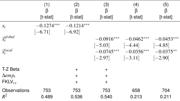
Table 7: Capitalization Rate Regressions

The dynamics of long-run prospects seem to be a key driver of real estate dynamics. As seen in sections (5) and (7), the link has both a expected return and cash flow component. This table reports the results of regression (6), which empirically answers which process dominates. The capitalization rate data is from Integra Realty Resources. I cluster along both the time and MSA dimension. Model (1) runs the regression on the full sample of capitalization rates for urban multi-family home property types. Model (2) adds the contemporaneous business cycle variables from section (4). Model (3) splits my measure of long-run prospects into its global and local components. Model (4) and (5) seek to mitigate spurious correlation issues as both the dependent and independent variables are highly per-sistent. I first difference the PS-ratios and measure of long-run growth prospects. That is, I regress the annual change in capitalization rate onto the change in local prospects (see equation (7)). Mod-els (4) does this regression on urban multi-family home capitalization rates; model (5) on suburban multi-family home capitalization rates. Both regressions are still clustered along the time dimension.

(1) (2) (3) (4) (5)

β [t-stat]

β [t-stat]

β [t-stat]

β [t-stat]

β [t-stat]

x_t −0.1274∗∗∗ −0.1214∗∗∗

[−6.71] [−6.92]

b

x_tglobal −0.0916∗∗∗ −0.0462∗∗∗ −0.0453∗∗∗

[−5.03] [−4.44] [−4.85]

b

x_tlocal −0.0745∗∗∗ −0.0356∗∗∗ −0.0375∗∗

[−2.97] [−3.11] [−2.90]

T-Z Beta + +

∆empt + +

FKLVcs + +

Observations 753 753 753 658 704

R2 0.489 0.536 0.540 0.213 0.211

data; to the degree that expectations will be immediately embedded in the surveyed price-to-rent ratios, the contemporaneous regression presented in equation (6) will even better mitigated this possible issue. Second, my return measure from earlier does not include rental income and is thus not a proper martingale. The capitalization rate data implicitly includes a measure of rent.

employ-ment growth and business cycle beta, and credit supply. As with the return regressions, both load on these regressions, but their economic impact is smaller than that of long-run prospects. Col-umn (3) splits my measure of long-run prospects into its global and local components. Similar to my return regressions, both components load significantly in the expected direction. As Plazzi, Torous and Valkanov (2010), highlight from their capitalization rate data, the cross-sectional vari-ation in cap rates is much greater then the time series varivari-ation. Given the high degree of per-sistence, especially in panel, of both the right and left sides of equation (6) there is concern that these results could be spurious. As robustness, I first difference the MSA-level PS-ratios and measure of long-run local growth prospects. That is, I’m seeing how the price-to-rent (ps_t) ratios change with local prospects,

∆psmsa,t =bglobal∆xglobalmsa,t +blocal∆xlocalmsa,t+εmsa,t. (7)

6

ECONOMIC FOUNDATIONS

In this section, I develop a representative agent model that helps account for my empirical find-ings. First, the decision to build and the process of consuming local specific housing services in-volve horizons that are longer than the duration of a typical business cycle fluctuation. My agent’s post-trade endowment is thus exposed to a low volatility, highly persistent state variable that seeks to reflect the dynamics of my local measure of long-run growth prospects. To properly internalize the risk to their wealth from the dynamics in long-run prospects, my agent has recursive prefer-ences (see Bansal and Yaron (2004)).

Second, my empirical findings in section (5) suggest that when the economic environment is bad - i.e. expectations of future cash flow is low - for firms located within an MSA, the expected risk premia of housing decreases. This implies that housing acts as a hedge to poor long-run growth prospects. In my model, the location specific consumption provided by housing is thus highly durable to the downside. This downside protection generates a regime switching dynamic in the expected excess returns to housing. The transition between these states is gradually in-creasing in my state variable as it is a function of the probability of being in a high growth state tomorrow given the growth state today. This setup allows me to replicate my empirical findings and then motivates a more in-depth empirical analysis of underlying consumption behavior in section (7).

6.1 Setup of the Economy

housing (S_t) and non-housing (C_t) goods

U_t = (1−β)ln(ut) +βlnEt[exp(θUt+1)]θ, where (8)

ut =

(1−α)C ε−1

ε t +αS

ε−1

ε t

_ε−ε₁

,

whereθ = ₁₋1

γ and is a function of risk aversion,γ,εis the intra-temporal elasticity of

substitu-tion, andαcaptures the agents relative preference for housing versus non-housing consumption. I choose to limit my analysis to unitary IES as this corresponds to the average number estimated in the empirical literature and several theoretical studies have already employed this specification (e.g., Tallarini (2000); Colacito, Ghysels, Meng and Siwasarit (2016)). Epstein and Zin preferences have been used extensively in RBC models to explain asset pricing puzzles although the analysis as been largely limited to equities, bonds, and their derivatives (e.g., Bansal and Yaron (2004); Co-lacito and Croce (2011); Gomes, Kogan, Yogo (2009); Eraker, Shaliastovich, and Wang (2016)). Fillat (2008) uses a similar setup as mine with housing assets being priced, but largely focuses on its impact on equity and bond prices.

By separating the risk (captured byθ) from inter-temporal consumption decisions (captured by IES), EZ-preferences provide a channel through which a MSA’s long-run industry prospects play an important role in an agent’s consumption behavior. This is illustrated by the additional variance term if I assume the agents wealth follows a log-normal distribution,

U_t = (1−β)ln(ut) +βEt[Ut+1] +β 1

2θVt[Ut+1]. (9)

I complete my local economy by specifying an endowment process for the MSA’s non-housing good and housing service consumption growth. Both contain exposure to a AR(1) predictive com-ponent,xt. In my monthly calibration the persistence coefficient,ρ, is close to but still less than

one, and matches the average persistence of my empirical measure of local long-run growth prospects. I assume that the endowment of both goods is a function of the same underlying state variable,x_t. This is similar to Gomes, Kogan and Yogo (2009), who assume a single aggregate productivity measure drives production for both non-durable and durable goods manufacturing firms.

∆ct+1=µc+φcxt+ λ

2(st−ct) +σcec,t+1, (10)

∆st+1=µs+Ix>0φsxt− λ

2(st−ct) +ϕsσces,t+1, where

x_t=ρxt−1+ϕxσcεx,t.

µ_candµ_sare the unconditional growth non-housing consumption and housing service endow-ments,φcandφsare leverage exposures to underlying local prospects. The first and second equations in system (10) also include a co-integration term, λ₂(st−ct). As highlighted by Piazzesi, Schneider and Tuzel (2007), housing as a share of total expenditures has stationarity proper-ties over my sample horizon; this is not the case, for example, with durable versus non-durable goods consumption. My no-bubble condition links non-housing and housing services consumption across time to maintain this property (see Giglio, Maggiori and Stroebel (2016) for further discus-sion on the existence of bubbles in housing markets). The parameterλdetermines the rate of convergence of the relative quantities. In addition, I assume that the shocks in system (10) are standard normal and orthogonal.

agglom-eration. Thus, in my model, while the endowment of non-housing goods is symmetrically exposed toxt(following Bansal and Yaron (2004)), housing services can expand in “good” times, which is activated by the indicator variable_Ix>0, but not contract in “bad.” Given thatxt is a mean zero pro-cess, the kink resides atxt =0. The assumption of a hard kink is admittedly extreme; however, the model captures the more general idea that in bad times housing services cannot contract at the same rate as non-housing consumption. That is the relative, not absolute, durability of housing services is what is important from a pricing perspective.

6.2 Financial Markets and Equilibrium of the Economy

My empirical setup effectively assumes that each MSA acts in autarky for both consumption goods - i.e. the representative agent in each MSA consumes only the good with which he is en-dowed. If the implied prospects of the local industry mix is high, this is immediately reflected in the consumption endowments locally for both non-housing goods and housing services. This setup can be motivated as a segmented or post-trade economy.

As I allow long-run prospects and thus the composition of consumption (lnSt

Ct =sct) to be

con-ditioned on past values, bothx_t andsc_t are state variables. I solve for equilibrium of my utility func-tion and price-to-consumpfunc-tion ratios using standard iterafunc-tion methods along a 3σgrid ofx_t and

sc_t. Expectations are computed across a 99-point gaussian quadrature, which randomly assigns shocks fore_c,e_s, andεx(see details of algorithm and derivations in APPENDIX G).

Using the non-housing good as the numer ´eaire, the stochastic discount factor is characterized by

M_t+1=

βexp(Ut+1/θ)

Etexp(Ut+1/θ)

u_t+1 ut

1

ε−1C

t+1

Ct −1

ε

. (11)

aggregated bundle of non-housing goods and housing services and is thus a composition growth risk term. Given that both non-housing and housing service endowment growth is a function of highly persistent terms, the continuation utility (first) term is impacted by both risks in the SDF.

I then use the Euler equation,Et[Mt+1Rs,t+1] =1, to pin-down expected excess returns for the local housing. For the housing asset, the price-to-rent,lnPs,t

st , is

lnPs,t

s_t =pst=lnEt[exp(mt+1+log(exp(pst+1) +1) +∆st+1)]

where lower cases signify logs (see APPENDIX G for explicit recursive formulations). Given the value functions of the price-to-rent, both the excess return,r_s,t+1=ln(exp(pst+1) +1)−pst+ ∆st+1, and excess price appreciation,rs,t+1 = pst+1−pst+∆st+1, can be computed for local housing.

I assume that the aggregate, or non-segmented markets, are priced by a subset of people that are not tied down to the location of housing services. That is they can allocate or trade housing between multiple MSAs. One could think of these individuals as represented by representative institutional money manager or a wealthy individual. I show in APPENDIX H that this representa-tive agent then prices aggregate markets as in Bansal and Yaron (2004) with long-run risk and stochastic volatility. Given this result, my empirical strategy immediately follows. I can identify

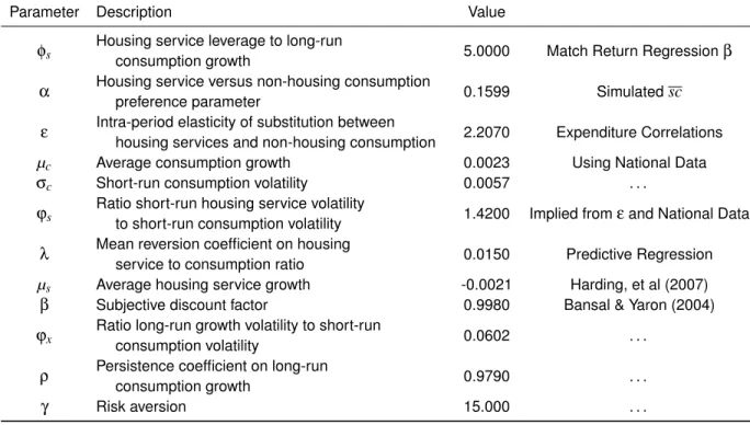
Table 8:Model Calibration

This table reports the calibration used in my model.β,ρ,ϕx, andγare taken from Bansal and

Yaron (2004). The utility weight parameter,α, on housing services is estimated as in Gomes, Kogan and Yogo (2009). The elasticity of substitution between non-housing goods and housing service con-sumption,ε, is estimated from theβwhen regressing expenditures of housing onto expenditures of

non-housing goods.µc,µs,ϕs, andλare estimated from aggregate housing to non-housing

consump-tion data.φsis a free variable that is calibrated to match my empirical results from section (5).

Parameter Description Value

φs Housing service leverage to long-run

consumption growth 5.0000 Match Return Regressionβ

α Housing service versus non-housing consumption

preference parameter 0.1599 Simulatedsc

ε Intra-period elasticity of substitution between

housing services and non-housing consumption 2.2070 Expenditure Correlations

µc Average consumption growth 0.0023 Using National Data

σc Short-run consumption volatility 0.0057 . . .

ϕs

Ratio short-run housing service volatility

to short-run consumption volatility 1.4200 Implied fromεand National Data

λ Mean reversion coefficient on housing

service to consumption ratio 0.0150 Predictive Regression

µs Average housing service growth -0.0021 Harding, et al (2007)

β Subjective discount factor 0.9980 Bansal & Yaron (2004)

ϕx

Ratio long-run growth volatility to short-run

consumption volatility 0.0602 . . .

ρ Persistence coefficient on long-run

consumption growth 0.9790 . . .

γ Risk aversion 15.000 . . .

6.3 Calibration of the Model

Table (8) provides the monthly parameter values for my model. The parameters are chosen at a monthly frequency in the spirit of work done by Bansal, Kiku, and Yaron (2012), who esti-mate the decision frequency of agents in their economy to be roughly one month. The subjective discount factor (β), persistence on long-run prospects (ρ), relative variance of long-run to non-housing consumption shocks (ϕx) and risk aversion coefficient (γ) are taken directly from Bansal and Yaron (2004). I equate the average housing service growth (µ_s) to depreciation; Harding, Rosenthall and Sirmans (2007) estimates that housing depreciates at roughly -2.5% per year.

compo-nent of the local stochastic discount factor (SDF) that determines excess housing returns. Coming directly from the endowment equations (10), I can compute the level of this quantity,

logSt+1

Ct+1

=sc_t+1= (1−λ)sct+µ+ (φs−φc)Ix>0xt−φcIx<0xt+esc,t+1. (12)

NIPA provides quantity estimates which I can use to estimate this regression; however, the Bu-reau of Labor Statistics’ (BLS) process of splitting housing expenditures into quantities and prices is fraught with error. For example, Boskin, Dulberger, Gordon, Griliches, and Jorgenson (1998) discuss the historical inconsistencies in how the BLS estimates housing services (quantities) and rent (prices) due to changing surroundings and technology - e.g., agglomeration economies, pol-lution and widespread use of electricity. To avoid these issues tainting my calibrations, I follow Piazzesi, Schneider and Tuzel (2007) in using expenditure rather then price or quantity data to estimate parameters.

This is straightforward given that prices and quantities of my assets are linked via the intra-period equilibrium. Assuming that non-housing is the numer ´eaire,

u_s,t u_c,t

= p s t p_tc =

α

1−α

S_t C_t

−1 ε

.

I define relative expenditures of housing services and non-housing goods as

ωt=ln p_tsS_t pc_tC_t =ln

Shelter

Total Expenditure - Shelter, (13)

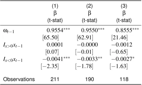
expres-Table 9:Aggregate Calibration Regressions

This table reports the regression results of equation (14) using aggregate expenditure NIPA data on an annual basis. The dependent variable is log housing to non-housing expenditures. All indepen-dent variables are standardized so that expressions represent a one standard deviation change. Model (1) uses all available data. Model (2) removes the boom-bust of the financial crisis, i.e. data post 2005. Model (3) uses data from 1960 to 2005. Standard errors are Newey-West corrected with a lag of 4. Given the annual frequency of the data, coefficients must be scaled when used as parameter estimates for my monthly calibration. *, **, and *** denote significance at the 10%, 5%, and 1% levels.

(1) (2) (3)

β

(t-stat)

β

(t-stat)

β

(t-stat)

ω

0

.

9554

0

.

9550

0

.

8555

[

65

.

50

]

[

62

.

91

]

[

21

.

46

]

I

x

0

.

0001

−

0

.

0000

−

0

.

0012

[

0

.

07

]

[

−

0

.

01

]

[

−

0

.

65

]

I

x

−

0

.

0041

−

0

.

0033

−

0

.

0027

[

−

2

.

35

]

[

−

1

.

78

]

[

−

1

.

63

]

Observations 211 190 118

sion for an OLS regression I run on national NIPA data at an annual frequency,

ωt=µ+ (1−λ)ωt−1+

1−1

ε

(φs−φc)Ix>0xt−1−

1−1

ε

φcIx<0xt−1+

1−1

ε

esc,t. (14)

Given the extremely lowλ, housing to non-housing consumption is also extremely persistent. Correlation in expenditures of housing services and non-housing goods consumption should be dominated by the higher volatility i.i.d. shocks in system (10). I can thus estimate the elasticity of substitution (ε) via the covariance of growth in housing to non-housing expenditures in the data. From the intra-period CES aggregator,

ln

_ps t+1St+1

ps_tS_t

=

1−1

ε

∆st+1+

1

ε∆ct+1

The inverse of theβcoefficient of expenditures will thus be my estimated value ofε. My es-timate of 2.2070 is close to that eses-timated in the literature (see Piazzesi, Schneider and Tuzel (2007)).

Given that non-housing consumption is my numer ´eaire and the orthogonality of short-run shocks, I extract estimates of non-housing and housing consumption dynamic parameters (µ_c, σcandϕs) directly from the data. I compute an estimate of the ratio of short-run housing service to short-run non-housing consumption volatility from the volatility of the expenditures ofsct. My model assumes thates,t+1is orthogonal toec,t+1;ϕsis therefore

p

σ2_sc−σ2_c/σc. Finally, using the approach of Gomes, Kogan and Yogo (2009), I estimate the housing to non-housing consump-tion preference parameter (α) from the mean aggregate expenditure ratio in the data and the men housing to non-housing quantities from my model. The remaining free-parameter,φs, is calibrated by matching the slope coefficients from my price appreciation empirical analysis in section (5).

6.4 Numerical Results

shows that this is in fact the case.

Both equilibrium figures also show the contours of the two risk regimes. When growth prospects are extremely high housing is exposed to two sources of risk (short- and long-run), but only one when prospects are extremely low. At the two extremes, expected excess returns and price ap-preciation are effectively constant. Without recursive preferences the transition between regimes would be immediate. The elongated transition zone from the low return to high return regime thus allows for empirical identification of the positive relationship between long-run growth prospects and expected excess price appreciation. During the time frame of our regressions, roughly 1975-2011, local long-run prospect, across all MSAs, were roughly0.45σabove the mean over the longer CRSP industry PD-ratio sample. In addition, the shocks to local prospects, assuming the AR(1) construct from my model, are approximately 80% correlated across MSAs. This implies that the relationship betweenr_tp₊₁andx_t is squarely in this elongated zone during the sample from my empirical exercise. In addition the relationship is well identified because of the large cross section of MSAs.

To replicate the regressions in section (5), I simulate 375 MSAs over 40years on a monthly basis at the 1975-2011 mean of long-run growth prospects and correlation of shocks. I then ag-gregate the simulatedxmsa,t, psmsa,t andr_msap _,t+1on an annual basis and run the same pooled coefficient regressions from section (5.1) and (5.3) on the simulated data, respectively

r_msap _,t=b_xx_msa,t−1+εmsa,t, and p_t−s_t=βxxt+ +εmsa,t.

Figure 2: Equilibr ium Pr ices and Empir ical Replication Figure (2A) is the equilibr ium e xpected retur n of housing giv en the state v ar iab le , xt , from m y model. My reg ressions from section (5) w ere on pr ice appreciation measure; figure (2B) presents the equilibr ium pr ice appreciatio n. Dur ing the per iod of m y sample of housing retur ns , xt w as on er age 0 . 45 σ higher than a v er age o v er the full, 1947-2011, CRSP sample . In addition, assuming the AR(1 ) process from m y model, shoc ks to long-prospects are on a v er age 80% correlated in m y sample . I sim ulate 375 MSAs o v er 40y ear s on a monthly basis around this histor ically high mean correlation. I then agg regated the sim ulated xmsa , t , ps msa , t and r p msa , t + 1 on an ann ual basis and run predictiv e reg ressions similar to those in m y ical e x ercise . Figure (2C) is the distr ib ution of bx for each MSA. The pooled coefficient is represented b y the b lac k line . T ab le (2D) are the results the tercile (model (1)) and supply elasticity (model (2)) reg ressions from section (6. 5). A: Expected Excess Retur n -6 -4 -2 0 2 4 6 xt # 10 -3 0 0.005 0.01 0.015 0.02 0.025 E t [r ex msa,t+1 ] B: Expected Excess Appreciation -6 -4 -2 0 2 4 6 xt # 10 -3 -0.031 -0.025 -0.019 -0.013 -0.007 E t [r p msa,t+1 ] C: Empir ical Replication -0.002 0.006 0.014 0.022 0.03 bx 0 0.05 0.1 0.15 0.2 0.25 0.3 Frequency D: Fur ther Implications Itr 1 ·

xt−

1 0 . 0127 ∗∗∗ [ 2 . 83 ] Itr 2 ·

xt−

1 0 . 0183 ∗∗∗ [ 5 . 23 ] Itr 3 ·

xt−

1 0 . 0143 ∗∗∗ [ 5 . 61 ]

xt−

1 0 . 0122 ∗∗∗ [ 4 . 49 ] log ( ηmsa ) ·

xt−

regressions in section (5.3). With this simple model I am able to closely replicate my empirical findings.

6.5 Further Empirical Implications

There are two additional empirical implications of my model. First, the relationship between long-run growth prospects and returns should not be linear. The sensitivity should be greatest when prospects are good, but low when prospects are either extremely good or extremely bad. To test this hypothesis, I run regression (4) with the full-set of controls described in section (5), but split the sensitivity of returns,b_x, into terciles ofx_t,

r_msap _,t =b1Itr1xmsa,t−1+b2Itr2xmsa,t−1+b3Itr3xmsa,t−1+Time FE+MSA FE+Controls+εmsa,t.

The results of the regression are in the first column of table (2D). Visually, although their eco-nomic difference is small, the difference in coefficient values fits the intuition developed from my model. Statistically, the differences in sensitivity is significant. A Wald test of equality between all three is rejected at a 10% level. The test statistic is largely driven by the rejection of equality of the coefficients of the second and third terciles, both of which are extremely well identified.

work.

In urban economics there is a rich literature relating house pricelevelsto elasticity. For exam-ple, Saiz (2010) generates empirical measures of MSA-level elasticity that embed both the phys-ical and regulatory components of elasticity. As my analysis is looking at the risk-return tradeoff, I’m interested in changes to the degree of predictability of long-run prospects on expected housing returns given different levels of housing elasticity. I thus add the interaction of the Saiz measure, ηmsa, and long-run local prospects to regression (4) to test my hypothesis.

r_msap _,t=bxxmsa,t−1+bsaizlog(ηmsa)xmsa,t−1+Time FE+MSA FE+Controls+εmsa,t