X-RAY SCATTER TOMOGRAPHY USING CODED APERTURES
Kenneth P. MacCabe
A dissertation submitted to the faculty at the University of North Carolina at Chapel Hill in partial fulllment of the requirements for the degree of Doctor of Philosophy in the
Department of Physics and Astronomy.
Chapel Hill 2014
© 2014
ABSTRACT
Kenneth P. MacCabe: X-ray scatter tomography using coded apertures (Under the direction of David Brady and Otto Zhou)
This work proposes and studies a new eld of x-ray tomography which combines the principles of scatter imaging and coded apertures, termed coded aperture x-ray scatter imaging (CAXSI). Conventional x-ray tomography reconstructs an object's electron density distribution by measuring a set of line integrals known as the x-ray transform, based physically on the attenuation of incident rays. More recently, scatter imaging has emerged as an alternative to attenuation imaging by measuring radiation from coherent and incoherent scattering. The information-rich scatter signal may be used to infer density as well as molecular structure throughout a volume. Some scatter modalities use collimators at the source and detector, resulting in long scan times due to the low eciency of scattering mechanisms combined with a high degree of spatial ltering. CAXSI comes to the rescue by employing coded apertures. Coded apertures transmit a larger fraction of the scattered rays than collimators while also imposing structure to the scatter signal. In a coded aperture system each detector is sensitive to multiple ray paths, producing multiplexed measurements. The coding problem is then to design an aperture which enables de-multiplexing to reconstruct the desired physical properties and spatial distribution of the target.
In this work, a number of CAXSI systems are proposed, analyzed, and demonstrated. One-dimensional pencil beams, two-dimensional fan beams, and three-dimensional cone beams are considered for the illumination. Pencil beam and fan beam CAXSI systems are demonstrated experimentally. The utility of energy-integrating (scintillation) detectors and energy-sensitive (photon counting) detectors are evaluated theoretically, and new coded aperture designs are presented for each beam geometry. Physical models are developed for each coded aperture system, from which resolution metrics are derived. Systems employing dierent combinations of beam geometry, coded apertures, and detectors are analyzed by constructing linear measurement operators and comparing their singular value decompositions. Since x-ray measurements are typically dominated by photon shot noise, iterative algorithms based on Poisson statistics are used to perform the reconstructions.
ACKNOWLEDGEMENTS
The author would like to thank the dissertation committee members for their generous patience and guidance. The previously published results were made possible by the hard work of a number of co-authors, specically:
Chapter 2: D. J. Brady, D. L. Marks, and J. A. O'Sullivan
Chapter 3: D. J. Brady, D. L. Marks, E. Samei, K. Krishnamurthy, and A. Chawla Chapter 4: D. J. Brady, D. L. Marks, M. P. Tornai, and A. D. Holmgren
I would also like to thank my friends and colleagues in the Duke Imaging and Spectroscopy Program and elsewhere who have oered their thoughts and experience, my parents Steve and Beth for raising me right and always encouraging me, my talented brothers Greg, Lee, and Ted who always treat me like a hero, and my loving wife Kat for her unwavering support in more ways than I ever thought possible. Also, I owe a great debt to our cats Bear and Foxy for humoring me during countless hours of practice presentations.
TABLE OF CONTENTS
LIST OF TABLES . . . ix
LIST OF FIGURES . . . x
LIST OF ABBREVIATIONS . . . xii
CHAPTER 1: INTRODUCTION . . . 1
1.1 Background . . . 1
1.2 Scatter imaging principles . . . 8
1.2.1 Scattering from a point . . . 9
1.2.2 Forward models for volume imaging . . . 16
1.3 Coded apertures . . . 17
1.4 Discretization of the forward model . . . 20
1.5 Reconstruction algorithms . . . 21
1.6 Singular value analysis . . . 23
CHAPTER 2: CODED APERTURES FOR X-RAY SCATTER IMAGING 26 2.1 Background . . . 26
2.2 Pencil beam CAXSI . . . 28
2.3 Anisotropic scattering . . . 30
2.4 Fan beam CAXSI . . . 34
2.5 Scalability of imaging techniques . . . 39
2.6 Summary . . . 40
CHAPTER 3: PENCIL BEAM CAXSI . . . 42
3.1 Background . . . 42
3.2 Forward model . . . 44
3.4 Reconstruction algorithm . . . 52
3.5 Results and discussion . . . 55
CHAPTER 4: FAN BEAM CAXSI . . . 62
4.1 Background . . . 62
4.2 Theory . . . 65
4.2.1 Forward model . . . 65
4.2.2 Reconstruction algorithm . . . 68
4.2.3 System design and resolution . . . 69
4.3 Experimental methods . . . 69
4.3.1 Conguration . . . 69
4.3.2 Acquisition . . . 70
4.3.3 Aperture fabrication . . . 70
4.3.4 Model calibration . . . 71
4.3.5 Test objects . . . 71
4.4 Results . . . 72
4.5 Summary . . . 77
CHAPTER 5: CODED APERTURES FOR VOLUME IMAGING . . . 79
5.1 Background . . . 79
5.2 Forward model . . . 81
5.3 Frequency scale codes (FSC) . . . 84
5.4 Scanning techniques . . . 87
5.5 Compressive sampling . . . 88
CHAPTER 6: ENERGY SENSITIVE CAXSI . . . 90
6.1 Background . . . 90
6.2 Resolution analysis . . . 92
6.3 Simulations . . . 94
LIST OF TABLES
LIST OF FIGURES
1.1 Basic elements of an x-ray tomography system . . . 2
1.2 Pencil and fan beam collimation . . . 4
1.3 Schematics of incoherent and coherent x-ray scattering mechanisms . . . 9
1.4 A simple x-ray scattering experiment . . . 10
1.5 Graphical denition of the momentum transfer q=pf −pi . . . 12
2.1 System geometry for planar scatter imaging . . . 27
2.2 Coded aperture based on the identity matrix . . . 32
2.3 Coded aperture based on the discrete cosine transform (DCT) . . . 32
2.4 Coded aperture based on a Hadamard matrix . . . 33
2.5 Coded aperture based on a random binary matrix . . . 33
2.6 Singular value spectra of the pencil beam system for each code choice . . . . 34
2.7 Coded apertures based on a sinusoid in x and a quadratic residue code iny . 36 2.8 Singular value spectra for each of the coded apertures in Fig. 2.7. . . 37
2.9 Random grayscale coded aperture . . . 38
2.10 Singular value spectra for the proposed code and a random code. . . 38
3.1 Schematic of a pencil beam coded aperture x-ray scattering experiment . . . 43
3.2 The XSPECT model for the illuminating x-ray spectrum . . . 48
3.3 X-ray image of the coded aperture . . . 49
3.4 Diraction images for powder samples . . . 52
3.5 Reconstructed scattering density for conguration (A) . . . 55
3.6 Reconstructed scattering density for conguration (B) . . . 56
3.7 Reconstructed scattering density for conguration (C) . . . 56
3.8 Reconstruction results for individual samples . . . 58
3.9 Reconstruction results for a combination of samples . . . 59
3.10 Comparison of modeled and experimental scatter measurements . . . 60
4.2 Coordinate system for a fan beam scattering experiment . . . 65
4.3 Photos of the test objects . . . 72
4.4 Scatter measurements for the plastic DUKE letters . . . 73
4.5 Reconstruction results for the plastic DUKE letters . . . 74
4.6 Reconstruction results for the clock . . . 76
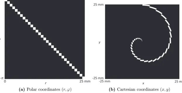
5.1 Relationship between the object, aperture, and measured spatial frequencies. 83 5.2 Coded aperture for volume tomography based on a ring structure in frequency 85 5.3 Measurable surfaces in the object space using a FSC . . . 86
5.4 Coded aperture for volume tomography based on a spiral structure in frequency 87 6.1 Pencil beam system geometry considered for energy sensitive CAXSI. . . 91
6.2 PSFs for energy sensitive measurements with and without a coded aperture . 93 6.3 Model for the incident x-ray spectrum . . . 95
6.4 Example impulse response for energy sensitive measurements. . . 96
6.5 PSFs for at energy spectrum compared with a tungsten spectrum. . . 97
6.6 Singular values for varying energy resolutions with/without a coded aperture 98 6.7 Singular vectors for ∆E = 128 keV without a coded aperture. . . 99
6.8 Singular vectors for ∆E = 128 keV without a periodic coded aperture. . . 100
6.9 Singular vectors for ∆E = 8 keV without a coded aperture. . . 101
6.10 Singular vectors for ∆E = 8 keV with a periodic coded aperture. . . 102
6.11 Singular vectors for ∆E = 8 keV with a random binary coded aperture. . . . 103
6.12 The 2D object used to simulate data for the reconstructions . . . 104
6.13 Simulated noiseless measurements for the random grayscale coded aperture. . 105
6.14 Reconstructed images from the simulated measurements . . . 106
LIST OF ABBREVIATIONS
m,s, eV, c Unit notation for meters, seconds, electron volts, speed of light in vacuum
CAXSI Coded aperture x-ray scatter imaging CSCT Coherent scatter computed tomography CT Computed tomography
DCT Discrete cosine transform
DE Dual-energy
DFT Discrete Fourier transform FSC Frequency scale code FZP Fresnel zone plate ME Multi-energy
MLE Maximum Likelihood Estimation (M)URA (Modied) uniformly redundant array SNR Signal-to-noise ratio
CHAPTER 1: INTRODUCTION
1.1 Background
The goal of tomography is to estimate physical parameters such as the electron density at each point in a three dimensional object [1]. Since x-rays provide penetration through other-wise opaque targets, x-ray tomography is an established eld for non-destructive examination and is widely used in medicine, security, and quality inspection. The primary contributions of this work are new modalities for tomography, enabled by reuniting coded apertures with x-rays through scatter imaging. These techniques are collectively termed coded aperture x-ray scatter imaging (CAXSI). An enabling feature of CAXSI is the design of a new family of coded apertures called frequency scale codes which provide maximum distinguishability of scatter points at dierent ranges from a detector. For a review on imaging modalities in x-ray tomography without coded apertures, see Reference [2].
The most popular and mature x-ray techniques operate in attenuation mode, where some fraction of the x-rays illuminating a target object are absorbed or deected from the direct ray path connecting the x-ray source and detector. By denition, the measured photons in attenuation imaging are those which did not interact with the object and thus provide limited information. In scatter imaging, scattered photons are measured, providing a number of advantages and novel results which will be discussed presently.
density. Density imaging based on uorescence is also possible using the isotropic scattering models presented in later chapters, and since uorescence is based on atomic transitions it can reveal concentrations of atomic constituents if the transition energies are detectable. While uorescence probes atomic structure, coherent scattering exhibits interference eects between neighboring atoms which can tell us about molecular structure. This is the motivator for coherent scatter imaging, where diraction proles are estimated for each point in an extended object. In the following, you will see demonstrations and examples of x-ray tomography systems for density imaging based on incoherent scattering and for molecular imaging based on coherent scattering.
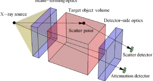
The basic model for an x-ray tomography system is shown in Figure 1.1 and consists of an x-ray source, beam-forming optical element(s), the target object, detector-side optical element(s), and detector arrays for attenuation and/or scatter measurements.
Figure 1.1: Basic elements of an x-ray tomography system, including the x-ray source, beam-forming optics, the target object volume, detector-side optics, and attenuation or scatter detectors.
class of reference structures, which partition the object into sensitivity regions specic to each detector and enable tomography [3,4]. The source-side reference structures considered here are pinhole and slit collimators, respectively forming pencil beams and fan beams as shown in Figure 1.2. The exception is Chapter 5, which concerns volumetric scatter imaging with full cone beam illumination. In principle, a 3D object may be translated through the pencil or fan beam to scan its full volume. X-rays transmitted or scattered by the object encounter detector-side optics before reaching the detectors. For the attenuation detectors, these usually consist of anti-scatter grids which are angled collimators focused on the source to reject scattered radiation. Until recently, scatter measurements have employed similar collimators focused on individual object points. Unfortunately, most of the scattered signal is thereby wasted through absorption since the collimators only transmit a narrow range of angles.
(a) (b)
Figure 1.2: (a) Pencil beam and (b) fan beam collimation
However, none of these methods provide tomography along a single line without irradiating at least a planar section of the object and acquiring a sequence of images.
In contrast with attenuation imaging, scatter imaging benets from the natural diversity of scattered rays. For each ray incident on a scattering object, multiple scattered rays are produced in dierent directions. Exploited properly, this means that a linear or planar section of the target may be imaged in a snapshot (a single exposure of a detector array) without the need for moving parts or multiple sources. Careful selection of scattered rays is important for minimizing radiation doses and/or maximizing throughput in tomographic systems. The ability to perform 1D tomography with a pencil beam alleviates the need to irradiate neighboring regions. In Chapter 2, theoretical analysis of 1D and 2D scatter imaging techniques shows that they could provide signicant reduction in radiation dose compared with alternative methods.
The second challenge for attenuation systems is material discrimination. Attenuation provides density information and eective atomic number when dual-energy (DE) or multi-energy (ME) measurements are made via photon counting detectors and/or spectral ltering at the source or detector. For DE measurements, density and eective atomic number are the only measurable properties. For ME measurements, relative combinations of atomic numbers can be discerned but only if the absorption features (e.g. K-edges) or uorescence energies of the constituent atoms falls within the detection energy range. For many applications, these features occur at energies too low to suciently penetrate the target. Incoherent scattering has been used instead of attenuation for density imaging [2,814], and specialized Radon methods have also been proposed for cone beam incoherent scatter tomography [15]. Incoherent scattering, however, lacks information about chemical structure since each electron contributes independently to the incoherent scattered radiation.
at crystal lattice sites become polarized and emit dipole radiation at the same frequency as an incident eld. Interference from neighboring atoms produces a scattered intensity which can be a quickly-varying function of the scatter angle. This intensity is closely related to the spatial Fourier transform of the electron density, providing important information about the spatial arrangement of the atoms or molecules. Similar eects occur in liquids and amorphous solids as in crystals, but with more smoothly-varying scattered elds. The coherently-scattered (diracted) eld depends strongly on both the x-ray energy as well as the molecular structure of the target, and therefore provides a non-destructive chemical probe.
X-ray diraction for chemical detection is a mature eld [17, 18]. A typical diraction experiment involves a small, point-like target and 1D x-ray illumination. Energy resolution is achieved either by a narrow-band x-ray source or energy-sensitive detectors. Localization in energy and space simplies the relationship between the measurements and the chemical structure of the target.
Coherent scatter imaging is a relatively new eld in which scatter/diraction measure-ments are made over an extended volume to measure the spatial and chemical conguration of a target. Coherent scatter imaging systems fall into three basic categories: selected volume tomography (SVT) [13,1925], coherent scatter computed tomography (CSCT) [2630], and coded aperture x-ray scatter imaging (CAXSI) [3135].
CSCT can be achieved with 2D illumination and detector pixels collimated to individual lines of voxels. The wider acceptance angle of the collimators improves throughput compared with SVT. CSCT cleverly adapts the mathematical framework of CT, providing analytic image reconstruction and error bounds [36]. Like CT, however, CSCT requires rotational scanning and cannot be used for snapshot tomography.
The newest category of scatter imaging techniques is coded aperture x-ray scatter imaging (CAXSI) [3135]. The novelty of CAXSI is that the detector-side collimator is replaced by a coded aperture with a carefully designed transmittance pattern. The aperture is constructed with enough angular acceptance to measure scatter from any illuminated region of the object, so that each detector pixel is sensitive to a dierent combination of voxels. With a sucient number of linearly independent measurements the target may be reconstructed from the measurements. Measurement diversity may be achieved by any combination of adding detector pixels, changing the code pattern, moving the object, and/or moving the source and detectors. Using CAXSI, a 1D or 2D tomographic section of the object may be reconstructed from a snapshot and without unnecessary irradiation of adjacent regions. Additionally, SNR and throughput are improved since viable aperture codes exist with average transmittance of about 50%. The scatter signal acquired in a CAXSI system is one and two orders of magnitude larger than with CSCT and SVT, respectively. CAXSI powerfully combines coded apertures with x-ray scatter imaging to enable new imaging modalities and improvements in image quality, acquisition speed, and chemical specicity.
CAXSI, in which density and chemical structure is recovered from a single snapshot along a 1D pencil beam. This is extended in Chapter 4, demonstrating snapshot 2D tomography and building on the lessons of the pencil beam system. Chapter 5 extends the ideas of its preceding chapters and proposes new coded apertures and reconstruction algorithms for cone beam scatter tomography. Chapter 6 compares models for systems incorporating linear arrays of spectroscopic (energy-sensitive) detectors. Finally, Chapter 7 provides a summary of this work and an outlook on the future of CAXSI.
1.2 Scatter imaging principles
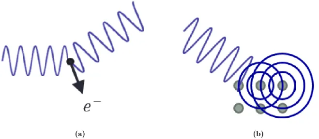
Photoelectric absorption, incoherent scattering, and coherent scattering are the dominant x-ray interactions with matter for photons in the 1 keV to 1 MeV energy range [37]. Figure 1.3 illustrates the two scattering mechanisms considered here. Incoherent scattering arises when a free or weakly bound electron absorbs energy from a photon and recoils. The energy transfer produces a shift in the photon's wavelength, known as the Compton shift. The amount of energy transferred to the electron is a random variable in this quantum process, but it is correlated with the scattering angle through energy and momentum conservation.
(a) (b)
Figure 1.3: Schematic representations of the two dominant x-ray scattering mechanisms considered here: (a) incoherent (Compton) scattering, and (b) coherent (Bragg) scattering. The sinusoids represent incident and scattered plane-waves. The e− in (a) is a scattered electron. The gray circles in (b) are atoms positioned on a crystal lattice, and the concentric rings are contributions from each atom to the scattered eld.
The scattering cross section σ is well approximated by a superposition of the individual cross sections: σ=σP+σI+σC, whereσP is for photoelectric absorption,σI is for incoherent
scattering, and σC is for coherent scattering. These cross sections are functions of the
photon energy E and have been measured and tabulated for a variety of materials [38]. The angular dierential cross section dσ
dΩ(θ, φ)is an even more complete description of a material's scattering properties and dened such that σ = dΩddΩσ(θ, φ). The solid angle element is dΩ = sinθdθdφ, and the polar angle θ is called hereafter the scatter angle, with θ = 0
being the direction of the incident illumination. Like σ, the dierential cross section also depends on E. In the following section, scatter measurements will be described in terms of the incoherent dierential cross section dσI
dΩ and the coherent dierential cross section dσC
dΩ . 1.2.1 Scattering from a point
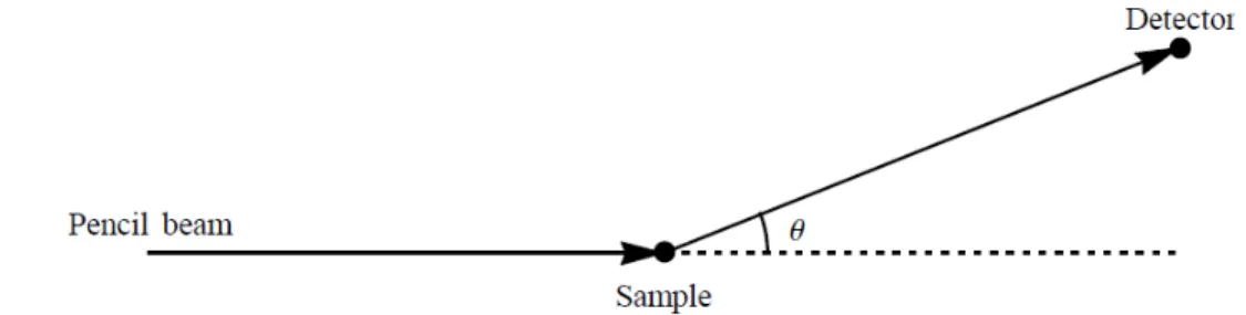
Figure 1.4: A simple x-ray scattering experiment, including a pencil beam, a point-like sample, and a spectroscopic scatter detector.
A pencil beam with spectral number density N(E) illuminates a point-like sample with
thicknessz and electron densityn, which scatters rays into multiple directions. The detector is assumed to cover an innitesimal solid angle Ω and positioned so that only x-rays with
scatter angleθare measured. The detector operates in photon counting mode, and adds each count to the appropriate energy bin. This is an example of an energy sensitive detector (Chapter 6 analyzes the performance of CAXSI systems employing arrays of such detectors). Letting ηi(E) be the probability that a detected photon with energy E is added to bin i,
the mean number of photons collected in energy bini may be represented as a contribution from incoherent and coherent scattering:
gi = znΩ
dE N(E)
ηi(E0)
dσI
dΩ(E, θ) +ηi(E) dσC
dΩ (E, θ)
. (1.1)
Equation (1.1) is called the forward model for the point scattering experiment. The par-ticulars of the energy and angle ranges measured, as well as the target's material properties, will determine which of these terms is dominant for a given measurement. The short x-ray wavelength compared with the periodicity of atoms in molecules causes coherent scattering to occur primarily in the forward direction at smallθ. Incoherent scattering, however, is found at allθ, and is relatively smoothly varying in energy and angle. The dierential cross section for incoherent scattering is well approximated by the Klein-Nishina formula [40], which has a peak at θ = 0 and another at θ = 180◦. In equation (1.1), E0 = E/1 + mcE2 (1−cosθ)
wheremc2 is the rest mass energy of the electron. Pencil beam tomography using incoherent scattering is possible with a single pixel and without detector side collimation by using energy sensitive detectors to ndθthroughEandE0[8]. However, for energy integrating detectors (those without energy resolution),ηi(E0)≈ηi(E) and the Compton shift is not resolved. In
this case, tomography is possible only through SVT or CAXSI, with signal strength being the advantage of the latter. Energy integrating detectors, based on scintillation or direct detection, will be assumed for Chapters 2-5.
The coherent scatter dierential cross section dσC
dΩ carries information about the spatial distribution of the electron charge, which may be used to identify the scattering material. Relaxing the assumption of a point-like target just slightly, letn(r)be the target's electron
density as a function of positionr. For an incident eld with wavevector ki proportional to
eiki·r, the phase at scattering point r is k
i·r. The amplitude of the scattered wave from
pointr is proportional to the electron density n(r). The scattered wave with wavevectorkf
suers a phase lag of −kf·r relative to the point r. The total scattered eld at wavevector
kf is a volume integral over n(r), with the phase factor ei(ki−kf)·r [16]:
E(kf) =
d3rn(r)ei(ki−kf)·r,
to within some proportionality. The spectral irradiance of the eld is proportional to
|E(kf)|2, motivating the following denition for the scattering density:
F(q) =
d3re−iq·r/~n(r)
2 ,
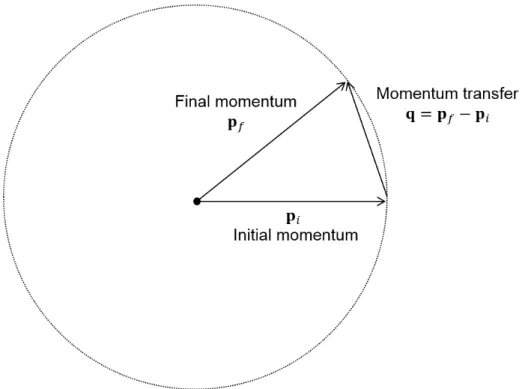
where the vector q = ~(kf −ki) is called the momentum transfer, and ~ is the reduced
Planck constant. Jumping from the wave picture to a particle description, an incident photon has the momentum vector pi = ~k and after scattering its nal momentum is pf = ~kf.
The momentum transfer q = pf −pi is the momentum gained by the photon during the
Figure 1.5: Graphical denition of the momentum transfer q = pf −pi. For coherent
scattering, |pf|=|pi| and both vectors lie on the surface of a sphere (the Ewald sphere).
In component form, the initial and nal photon momenta are
pi =
E c
0
0
1
pf =
E c
sinθcosφ
sinθsinφ
cosθ
|pi|=|pf|=E/c. The components of the momentum transfer q=pf −pi are
q = E
c
sinθcosφ
sinθsinφ
cosθ−1
(1.2)
The magnitude q of the momentum transfer vector gives us Bragg's law
q = 2E
c sin θ
2, (1.3)
relating the momentum transfer magnitude q, x-ray energy E, and the scatter angle θ. Equation (1.3) describes only the rst diraction order M = 1; higher orders are obtained
by multiplying the left hand side by the order number M. In what follows, all diraction orders except the rst are ignored.
In crystals, F (q) is nonzero only when q/~ is approximately equal to a reciprocal lattice vector. For a crystalline powder, averaging F (q) over the random distribution of
grain orientations produces a scattering density depending only on the magnitude q of the momentum transfer. This approximation breaks down as the grain size increases, but the simplication is even more exact for liquids and amorphous solids. Then, the scattering density is reduced to a function of a single parameter, F (q), and the scattered radiation
is said to possess azimuthal symmetry (it is independent of φ). Azimuthally symmetric scattering is analyzed in Chapter 2 and assumed in the forward models for coherent scatter imaging in Chapters 3, 4, and 6. The approximation F(q) ≈ F(q) is justied when the
spatial imaging resolution is much larger than the length scale at which the material is disordered.
The dierential cross section dσC
dΩ(E, θ) and the scattering density F q= 2E
c sin
θ
2
as
dσC
dΩ (E, θ) = A(E) 1 + cos
2θ
F
q= 2E
c sin θ
2
(1.4)
whereA(E)is a normalization factor for eachE so that dΩdσC
dΩ (E, θ) = σC(E), and σC(E) is the total coherent scatter cross section, e.g. as reported by NIST [38]. Appendix A discusses this normalization and how to compute F (q) and dσC
dΩ (E, θ) for arbitrary q , E , and θ from diractometer measurements and knowledge of σC(E). The factor (1 + cos2θ)
in equation (1.4) is proportional to the Thompson scattering factor (the low energy limit), which arises since the scattered eld has two polarization components and one of them (the radial component) follows a cos2θ dependence for the intensity.
Bragg's relationship (1.3) between two experimental parametersE andθ and the object-specic parameterq enables multiple modalities for diraction measurements. Measurement of the scattering density at dierent q values is achieved by varying θ with xed E (angle-dispersive), or varyingE with xedθ (energy-dispersive). Because of the limited acceptance angle of the collimators, SVT requires energy dispersive measurements to recoverF(q) [22].
Both angle and energy dispersive measurements have been demonstrated in CSCT [26,28,30] and CAXSI [31,32,34,35] systems. Angle-dispersive CAXSI is the focus of Chapters 2, 3, and 4. There exists a continuum between angle-dispersive and energy-dispersive measurements in which both E and θ vary, which is analyzed in Chapter 6.
Some comments on simplifying the forward model (1.1) are in order. Small angle scattering is assumed for coherent scattering, so that cos2θ ≈ 1. Incoherent scattering is only considered for energy-integrating detectors, so ηi(E0) ≈ ηi(E), and it is treated as
approximately isotropic. The coherent and incoherent contributions may be grouped into a total scattering cross section according to σS =σI+σC:
gi = nzΩ
dE ηi(E)N(E)
dσS
Some dierent limits of this forward model enable dierent measurement strategies. First, assume a narrow-band source so that N(E) → δ(E−E0) and assume a perfect energy-insensitive detector with η = 1, where the index i has been dropped since there is only a single energy bin. The forward model in this case is
g = nzΩdσS
dΩ (E0, θ),
which essentially the forward model for SVT. Ifn is the unknown density of a given voxel in SVT, it can be recovered with an appropriate model forzΩdσS
dΩ (E0, θ). This was the approach of Lale for incoherent SVT [19]. To recover F(q) when coherent scattering is measured,
angle dispersive measurements would scan g(θ) to recover F(q) ∝ gθ = 2 sin−1h2qcE
0
i
. This approach is used in commercial diractometers for small, point-like samples at known locations.
For common broadband x-ray tubes, narrow-band spectra most easily achieved through heavy ltration, wasting much of the incident ux. If the source is broadband, recovery of F(q) from g(θ) results in a deconvolution problem which can be ill-posed. To overcome
this problem for coherent scatter SVT, Harding and Kosanetzky took the energy-dispersive approach [22]. Their energy-sensitive detector remained at a xed angleθ0and had a number of energy bins so that, eectively, g(E) was measured. The coherent scatter forward model
is then
g(E) = nzΩN(E)η(E)k(E)F
q= 2E
c sin θ0
2
(1.5)
and the scattering density was recovered through F(q) ∝ g
E = qc
2 sinθ0 2
1.2.2 Forward models for volume imaging
The principles of point scattering from the previous section can be assumed at each posi-tion in a 3D object, with the total measurements being a superposiposi-tion of the contribuposi-tions from each point. This superposition principle applies best to weakly attenuating/scattering objects where the primary scatter is a mere perturbation of the incident beam and the secondary scatter is a small perturbation of the primary scatter. In the remainder of this work, perturbations of the incident and scattered radiation are assumed negligible or otherwise corrected-for. The result is that the forward model becomes a linear transformation of the scattering density F.
The purpose of scatter imaging is to estimate some combination of physical properties, such as electron density and/orF(q), over the volume of the object. The imaging process may
be considered as a transformation H from the object's now spatially-dependent scattering densityF(r, q)to the measured eld G(r0, E), where r= (x, y, z)is a position vector in the
object, r0 = (x0, y0, z0)is a measurement position, q is the momentum transfer, and E is the measured photon energy. The job is to estimate F (the object) fromG(the measurements), given a system model H. In general, H may be a nonlinear transformation of F due to multiple scattering eects and/or attenuation of the x-rays within the object, however for simplicity a linear model is assumed in this work (with the exception of a bi-linear model in Chapter 4). The techniques described here may be extended to iterative update of a nonlinear H during the reconstruction process.
shape of the actual voxels. Energy-dispersive SVT measures the coherent scattering density viaF (r, q)δ3(r−s(t))→G(E, t). SVT may also employ pixel arrays to capture one or two spatial dimensions of F in parallel. CSCT rotates F(x, z, q) and obtains energy-integrated
measurementsG(x, y, t)or energy-sensitive measurementsG(x, E, t). SVT and CSCT both
employ detector-side collimation to limit the domain of F which is visible to each detector pixel. CAXSI provides an alternative approach using coded apertures with wide angular acceptance, increasing the fraction of the scattered radiation reaching the detectors.
Chapter 2 presents theory and analysis for incoherent and coherent CAXSI systems, including coded apertures for forward models with F(z) → G(x), F (z, θ) → G(x, y), and
F (x, z)→G(x, y). In Chapter 3, the coherent scattering density F(z, q) was reconstructed
from an experimentally-measured G(x, y), which is closely related to the transformation
F (z, θ) → G(x, y) discussed theoretically in Chapter 2. In Chapter 4, the object was
assumed separable as F(x, z)R(θ), where the radiance R(θ) included both coherent and
incoherent scattering. The functionsF(x, z)and R(θ)were both estimated from the
experi-mental imageG(x, y). In chapter 5, coded apertures are proposed for volumetric tomography
following F (x, y, z) → G(x, y, t). Chapter 6 compares forward models for energy sensitive
measurements according to the transformation F (z, q)→G(x, E).
1.3 Coded apertures
models presented in the following chapters assume a planar aperture, with an exception in Chapter 6 which requires modeling of the 3D aperture due to an energy dependent forward model. For each coded apertures system, resolution metrics are presented in terms of the smallest length scale of the aperture pattern, however it may be decided.
In spectroscopy, coded apertures have been used as early as 1949 [41] to overcome resolution versus throughput tradeos. By multiplexing signals together, spectra may be reconstructed with signal to noise ratio (SNR) superior to single slit diraction. From this concept the eld of Hadamard transform spectroscopy developed and has become a testament to the power of multiplexing [42]. Recent studies show that novel codes in combination with biased, nonlinear and/or decompressive estimators may provide a powerful tool for compressive sampling [4]. Coded apertures may also be viewed as light eld encoders that enable radiance measurement using irradiance detectors [43]. Building on studies of reference structures for compressive tomographic imaging [3, 44, 45], coded aperture snapshot spectral imaging (CASSI) was developed in 2007 to measure a 3D spatial-spectral scene from 2D measurements at visible and ultraviolet wavelengths [46, 47]. In 2009, an extension of this approach was proposed for compressive x-ray tomography [48]. In each of these examples, coded apertures are used to alleviate space-time-spectral trade-os and enable snapshot acquisition of data conventionally recorded sequentially. For sparse or compressible objects coded aperture multiplexing can improve system sensitivity and signal to noise ratio even when photon noise is dominant [49].
Reference [51] provides a good description of their approach and an application to gamma rays. Inspired by digital reconstruction, in 1968 Ables [52] and Dicke [53] each proposed correlational imaging in which pinholes are positioned randomly in 2D to form a coded aperture. By correlating the measured image with the pinhole pattern, the image can be reconstructed with higher SNR than a single pinhole can provide for the same resolution. Later work improved the design of these coded apertures by considering their correlation properties [5456].
Most of the coded apertures discussed above are types of shift codes and are well-suited for x-ray astronomy and other applications where the goal is transverse 2D imaging. An ideal shift code with transmittance T(x) will possess a correlational inverse Tˆ(x) such
that dx T(x) ˆT(x −a) = δ(a), where δ(· · ·) is the Dirac delta function. For incoherent
imaging, the transmittance is constrained to 0 ≤ T(x) ≤ 1 but Tˆ(x) can take any value
since it is applied digitally. However, object points at dierent ranges will produce dierent magnications of T(x), and the shift codes then lose their nice orthogonality properties.
When shift codes are applied to 3D objects, a slice at a certain depth may be put into focus but it will still contain background contributions from the other slices, preventing true tomography.
A central theme of this work is the use of scale codes based on sinusoid functions, which were chosen based on their distinguishability under magnication. For a scale code T(x),
there exists an inverse Tˆ(x) so that dx T(x) ˆT(xa) = δ(a − 1). Scale codes are used
1.4 Discretization of the forward model
The forward models considered here describe linear transformations between continuous elds. In practice, discretization occurs at the detector during the digital measurement process and at the object during digital reconstruction. In the following, the object-space coordinates are combined into the 4D vector x = (r, q) and similarly for the measurement
coordinates x0 = (r0, E).
Experimental measurements are modeled as random variables, with mean values given by discrete projections of the spectral irradiance G(x0). The measurements are modeled
according to detector response functions{Φi(x0)}i=1...M, whereM is the number of measured
values. The expected value of the ith measurement is g
i =
dx0Φi(x0)G(x0) , where the
integral extends over the support ofΦi(x0). A similar discretization for the object is possible
over basis functions {Ψj(x)}j=1...N, where N is the number of unknown object coecients.
The jth object coecient is f
j =
dxΨj(x)F (x). Here, orthonormal but not necessarily
complete bases for Φ and Ψare assumed.
An important consideration is that the measurement response functions are based on physical devices, however the object basis may be chosen to suit a particular problem since it is merely a computational construct. In truncated singular value decomposition [4], the object basis consists of the right singular vectors of H (singular value decomposition is discussed in Section 1.6 below). Choosing another object basis in whichF is compressible or sparse is the concept behind compressed sensing [57,58]. For compressible objects, shockingly few measurements are required to recover the function F with high delity, even in the presence of extreme noise. This revelation has led to a urry of activity in the past decade, applying compressive techniques in almost every eld of imaging, communications, and signal recovery [4].
The discrete forward model is
gi = N
X
j=1 fj
dr0Φi(r0)
=
N
X
j=1 Hijfj
g = Hf (1.6)
where the components of the forward matrixH are dened as Hij in going from the rst to
second line. The third line puts the model in matrix form, dening vectors g and f with components gi and fj, respectively. The result is a linear system with M equations and N
unknowns. In general, M 6= N and the inverse H−1 does not exist. Even if it does exist, estimating ˆf = H−1˜g, where g˜ is a noisy measurement of g, may amplify the noise and produce poor recovery of f. The solution is to develop reconstruction algorithms specic to the noise statistics, as discussed in the next section.
1.5 Reconstruction algorithms
Two basic classes of reconstruction algorithms exist: direct and iterative. For direct reconstruction, an approximate inverse H˜ is used in place of H−1. The estimated object is then ˆf = ˜Hg˜, where g˜ is the noisy data with mean given by g. CT, SVT, and CSCT, all
enable direct reconstruction with a linear estimator H˜. The second class of algorithms is
iterative, meaning that the estimate ˆf is the limit of a converging sequence updated at each
For simplicity, assume that the random error in each measurement is independent of the other measurements. The noisy data are drawn from a Poisson distribution,
˜
g ∼ Poisson (g+g0)
wherePoisson (v)is a vector of independent Poisson realizations with mean values given by
the vector v. The vector g0 is a background term, which is included for the experimental demonstrations in Chapters 3 and 4 since g0 = 0 is dicult to achieve experimentally. For simplicity, in the following derivationg0 = 0but this term is restored later for the appropriate derivations.
One may write the log-likelihood L in terms of a product of Poisson distributions for each measurement:
L = ln
M
Y
i=1 gg˜i
i e
−gi
˜
gi!
=
M
X
i=1
[˜gilngi−gi−ln ˜gi!] (1.7)
The function of any maximum likelihood algorithm is to maximize L with respect to the estimated object f. This should occur where the gradient vanishes:
∂L ∂fj
=
M
X
i=1 ∂gi
∂fj
˜
gi
gi
−1
= 0 (1.8)
The derivatives ∂gi
∂fj are precisely the components of the forward matrix H. In the case of
a nonlinear forward model, H should be updated along with g at each iteration. In vector form, equation (1.8) implies that
HT (˜g./g)
where g./g˜ is an element-wise division and 1 is a vector of ones the same size as g. Since the expression on the left is the identity, the object f is a xed point of the functionF(f) =
f.∗HTH(˜Tg./1g), where.∗is an element-wise multiplication. This suggests the xed point iteration
fk+1 = fk.∗
HT (˜g./gk)
HT1 , (1.9)
recalling that g˜ (and H in the nonlinear case) is a function of fk. The estimatefk+1 at the
(k+ 1)st iteration is obtained by inserting the estimate fk at iterationk into the right hand
side of (1.9) and computing gk from the forward model (1.6). Equation (1.9) is the basic
update equation for Poisson MLE, and is used throughout this work with some modications where appropriate. For the experiments that follow, f was initialized with a constant value.
1.6 Singular value analysis
The coded aperture transmittance, along with the physics of the scattering and propaga-tion, are embedded in the transformation H for a given measurement system. In general, H is not invertible, or its inverse is not easily obtained. However, depending on the structure of the forward model (and in turn the structure of the coded aperture), one can learn a great deal about the object F even if it cannot be uniquely determined. The properties of H determine which structures of F are measured most accurately.
The singular value decomposition (SVD) may be performed for any linear operator over continuous or discrete domains and provides a powerful tool for comparing measurement systems. Reference [4] discusses SVD analysis for computational imaging and related recon-struction methods, such as truncated SVD and Tikhonov regularization. The basic concept for system analysis is that measurement noise produces an eective singular value cuto below which the singular vectors, and thus F, are not reliably recovered.
{Sk}, where k = 1. . . Ns is an index. The continuous form of the SVD is written as
G(x0) =
Ns
X
k=1
Uk(x0)SkFk (1.10)
where Fk =
dxVk(x)F(x) is the projection of F(x) onto the basis function Vk(x), a
right singular vector. The functions Uk are the left singular vectors. The singular value
Sk is the amplitude for which the singular vectorVk(x)is represented in the measurements.
IfSk = 0 for some k, then the corresponding Vk(x)is a vector in the null space of H and is
never measured. In the presence of noise, G(x0) is the mean of a random eld and vectors
with small Sk may not be reliably recovered. Singular value analysis is therefore a critical
step in design of any linear measurement system.
The discrete version of the SVD is the matrix factorization H = USV†, where U and V are unitary matrices and S is diagonal with entries given by the singular values Sk. The
operator † is the matrix adjoint, or conjugate transpose. The left singular vectors are
the columns of U and the right singular vectors are the columns of V. Specically, the components of Uand V are
Uik =
dx0Φi(x0)Uk(x0)
Vjk =
dxΨj(x)Vk(x)
where i = 1. . . M indexes the measurements, j = 1. . . N indexes the object coecients, and k = 1. . . Ns indexes the singular values. Here, the functions {Φi} and {Ψj} are the
measurement and object bases of Section 1.4.
CHAPTER 2: CODED APERTURES FOR X-RAY SCATTER IMAGING
(Adapted from previously published work [33])
2.1 Background
The focus of this chapter is a theoretical analysis of tomography based on coded aperture x-ray scatter imaging (CAXSI). Pencil and fan beam geometries are studied here, and singular value decomposition (SVD) is used to compare coded aperture designs, and also to compare each CAXSI system with other tomographic strategies such as Radon imaging and selected volume tomography (SVT). Scatter imaging commonly relies on SVT using collimation lters at the source and at the detector [2]. CAXSI is a novel approach to scatter imaging that uses coded masks between the scattering object and the detector array. In the following, pencil beam CAXSI is shown to enable 1D tomography from a snapshot measurement (a single exposure of a detector array) by detecting a diversity of scattered x-rays. Later in this chapter, these ideas are applied to fan beam CAXSI, suggesting a new coded aperture design for planar snapshot imaging. The rst experimental demonstration of pencil beam CAXSI is presented in Chapter 3, and its success inspired the experimental fan beam CAXSI system of Chapter 4.
Singular value analysis is often used to evaluate the noise sensitivity of measurement systems and to quantify the number of components measured above the noise oor. SVD analysis is presented in Section 2.5 which nds that the singular values for CAXSI decay more slowly compared with other techniques as the image resolution is increased. This suggests possible improvements in dose requirements and/or signal to noise ratio for CAXSI systems.
Detector array Coded aperture
Object
Illumination plane
Figure 2.1: System geometry for planar scatter imaging
Scattered radiation from the illuminated object passes through a coded aperture placed a distance d in front of a 2D detector array. In contrast with collimation lters, the coded aperture allows rays from multiple directions to simultaneously illuminate each detector pixel. Increased photon eciency is the advantage of CAXSI relative to selected volume imaging. CAXSI owes its throughput and snapshot advantages to coded apertures with high average transmittance (50%), a number of which are presented here for pencil and fan beams, and in Chapter 5 for cone beam illumination.
Shift codes are well known in coded aperture imaging and provide resolution parallel to a detector array. The shift codes used here are based on quadratic residues. A novel result of this work is sinusoid functions used as scale codes due to their distinguishability under magnication, providing resolution in range from a detector plane. These sinusoid apertures are precursors to the more general frequency scale codes of Chapter 5.
coded aperture designs are presented in Section 2.3. A new coded aperture for fan beam illumination and isotropic scattering is presented in Section 2.4, and the scalability of CAXSI is compared with other tomographic strategies in Section 2.5. Results from this chapter are summarized in Section 2.6.
2.2 Pencil beam CAXSI
As a rst example of code design, suppose that a pencil beam illuminates a section of the target object distributed along thez axis. Our goal is to image the object's scattering density F(x= 0, y = 0, z), or simply F(z). The full volume may subsequently be reconstructed by
raster scanning.
Assume isotropic scatter to all detector positions, which approximates Compton (inco-herent) scattering or x-ray uorescence when attenuation is weak and the detector array subtends a small solid angle with respect to the object (this last assumption will be relaxed in Section 2.3). The detector elements lie in the z = 0 plane and measure the scatter. The
scatter visibility is modulated by a coded aperture a distancedfrom the detector plane. For simplicity, we assume a 1D coded aperture transmittance T(x), where xmay be a Cartesian coordinate or a radius from the pencil beam axis. The signal at coordinate xin the detector plane is
G(x) =
zmax d
F(z)T
x
1− d
z
dz. (2.1)
For simplicity, the system geometric response is omitted and the source is monochromatic. Estimation of F(z)from G(x) is enabled by judicious selection of T(x).
The coordinate transformation β = 1−d/z changes (2.1) to
M(x) =
1 0
˜
F(β)t(xβ)dβ, (2.2)
where F˜(β) = F(z =d/(1−β))d/(1−β)2 and we assume z
max d. Equation (2.2) is a scale transformation; inversion is straightforward if T(x)is orthogonal in scale.
vanishing correlation. The simplest choice forT(x)satisfying the requirements that0≤T ≤
1 is T(x) = [1−cos(2πux)]/2, whereu is the spatial frequency of the coded aperture. The measurement model is then
G(x) = 1 2
1 0
˜
F(β) [1−cos(2πuxβ)] dβ. (2.3)
Equation (2.3) is familiar as the forward model for the Fourier transform spectroscopy [4]. The singular vectors for this transformation are derived from the constant singular vector associated with the1operator and prolate spheroidal singular vectors associated with
the kernel cos(2πuxβ). Assuming that the support of G(x) is [0, D], the singular value
corresponding to the rst operator isNx =uD, which is the number of sinusoid periods that
are observed for a scatter point at ∞.
The singular vectors of the operator −(1/2) cos 2πuxβ supported over β ∈ [0,1] and
x∈[0, X]are the prolate spheroidal wavefunctionsψn(β)forneven [62]. The corresponding
singular values are √λnNx/2, where λn≈1 for n < Nx/2 and λn ≈0for n > Nx/2 [4].
The even prolate spheroidal functions are not orthogonal to the constant vector over[0,1]
but the much larger singular value associated with the constant vector means that the spaces spanned by the two operators approximate the space spanned by their sum. The singular decomposition space thus consists of a single vector with singular value Nx/2and Nx/2−1
secondary vectors corresponding to singular values √Nx/2.
The prolate spheroidal basis yields resolution elements of length 1/Nx distributed
uni-formly distributed overβ = [0,1]. Converting back to thezcoordinate, one derives resolution
∆z = z
2
Nxd
. (2.4)
This expression may be understood by noting that the location z of a single point scatterer is localized by observing u¯, the frequency of the sinusoid projected onto the detector. The
two point scatters separated by a distance ∆z lose orthogonality when ∆¯u ≤ 1/X due to the nite detector size X. Propagating this uncertainty to z through∆¯u = ∂∂zu¯∆z produces equation (2.4).
2.3 Anisotropic scattering
In the previous section, sinusoidal codes were shown to provide range discrimination under isotropic scattering. If a 2D detector is used, there is a redundancy of scattered rays which may be exploited to estimate features other than density along the 1D object. In this section we present such an example where a more general scattering model relaxes the assumption of isotropic scattering to allow dependence onθ, the polar scattering angle. This applies, for instance, to coherent scattering from liquids, powders, and amorphous compounds. In this case one may vary the code T(ϕ, ρ)as a function of angle ϕand radius ρ in order to image θ and z simultaneously. The forward model in this case is
T(ϕ, ρ) =
zmax d
F(z, θ)T
ϕ, ρ
1−d
z
dz (2.5)
with polar angle ϕ and radius ρ in the detector plane. Let r = ρ 1− d z
be the radius at which the ray connecting beam position z with detector radius ρ intersects the aperture plane. Transforming the integral in equation (2.5) from z to r, and dening F˜(r, ρ) =
ρd
(ρ−r)2F z =ρd/(ρ−r), θ= tan
−1 ρ−r d
, the forward model takes the simple form
G(ϕ, ρ) =
T(ϕ, r) ˜F (r, ρ) dr. (2.6)
Each radius therefore denes a subspace for the operator T(ϕ, r)(· · ·)dr and its matrix representation T. The elements of the discrete forward operator T are Hij =T(i∆ϕ, j∆r),
motivating numerical evaluation.
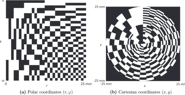
We seek invertible codes for T with entries in [0,1]. The simplest coded aperture is
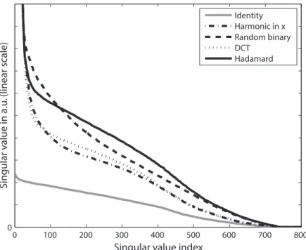
based on the identity matrix, shown in polar and Cartesian coordinates in Figure 2.2. This aperture is a type of collimator since each detector receives a single ray, and therefore provides minimal throughput. Multiplexing with 50% average transmittance can be achieved by a coded aperture based on a discrete cosine transform (DCT), shown in Figure 2.3. This mask contains grayscale values, but some applications require binary codes due to fabrication limitations. This motivates codes based on a Hadamard matrix (Figure 2.4) or randomized features (Figure 2.5). A high resolution Cartesian image of the DCT code is included which shows its continuous form, and the columns of the Hadamard matrix have been sorted so the angular frequency increases with radius. This sorting operation is unitary and therefore preserves the singular value spectrum.
For each of the apertures in Figures 2.2-2.5, the forward model (2.5) was numerically evaluated as a matrix in order to nd its singular value spectrum. The object was sampled with 48×48pixels from z =d to2d and θ = 0 to 27◦. Each coded aperture was simulated
at d = 100 mm with 31 polar sections and 31 radial sections from r = 0 to 25 mm. The
detector was sampled with 96 polar and 96 radial sections from ρ = 0 to 50 mm. The
singular value spectra for these code choices are plotted together in Figure 2.6, and this plot includes the sinusoid codeT(x)which was previously derived for isotropic scattering, labeled
0
-π π
25 mm
r φ
(a) Polar coordinates(r, ϕ)
25 mm
25 mm x
y
-25 mm -25 mm
(b) Cartesian coordinates(x, y)
Figure 2.2: Coded aperture based on the identity matrix
0
-π π
25 mm
r φ
(a) Polar coordinates(r, ϕ)
25 mm
25 mm x
y
-25 mm -25 mm
(b) Cartesian coordinates(x, y)
0
-π π
25 mm
r φ
(a) Polar coordinates(r, ϕ)
25 mm
25 mm x
y
-25 mm -25 mm
(b) Cartesian coordinates(x, y)
Figure 2.4: Coded aperture based on a Hadamard matrix
0
-π π
25 mm
r φ
(a) Polar coordinates(r, ϕ)
25 mm
25 mm x
y
-25 mm -25 mm
(b) Cartesian coordinates(x, y)
0 100 200 300 400 500 600 700 800 0 0.2 0.4 0.6 0.8 1 1.2 1.4 1.6 1.8 2 Identity Harmonic in x Random binary DCT
Hadamard
Singular value index
Si n gu la r v alue in a.u . (linea r sc ale)
Figure 2.6: Singular value spectra of the pencil beam system for each code choice
2.4 Fan beam CAXSI
CAXSI may also be applied to planar imaging. Once again, consider isotropic scattering for simplicity. When the entire yz plane is illuminated as in Figure 2.1, the forward model becomes
G(x, y) =
Y /2
−Y /2 zmax
d
F(x0 = 0, y0, z0)×T
x
1− d
z0
, y
1− d
z0
+y0d z0
dy0dz0. (2.7)
Choosing
T(x, y) = 1 + sin(2πux)p(νy)
2 , (2.8)
where p(νy) is described below, provides sensitivity to shifts in y and z. The quantity ν is the spatial frequency of the code in the y direction. Specically,
p(y) =X
n
where rect(y)is a unit square pulse of width 1 and {pn} is a binary sequence with two-level
auto-correlation. Such sequences may be found for various code lengths [63]. Quadratic residue derived codes of length P = 4m+ 1, withP prime, are particularly straightforward, and yield transverse imaging resolution ∆y = z/(νd) [56]. Two scatter points separated
by ∆y produce signals shifted by one code period in the y direction, which sucient for distinguishability.
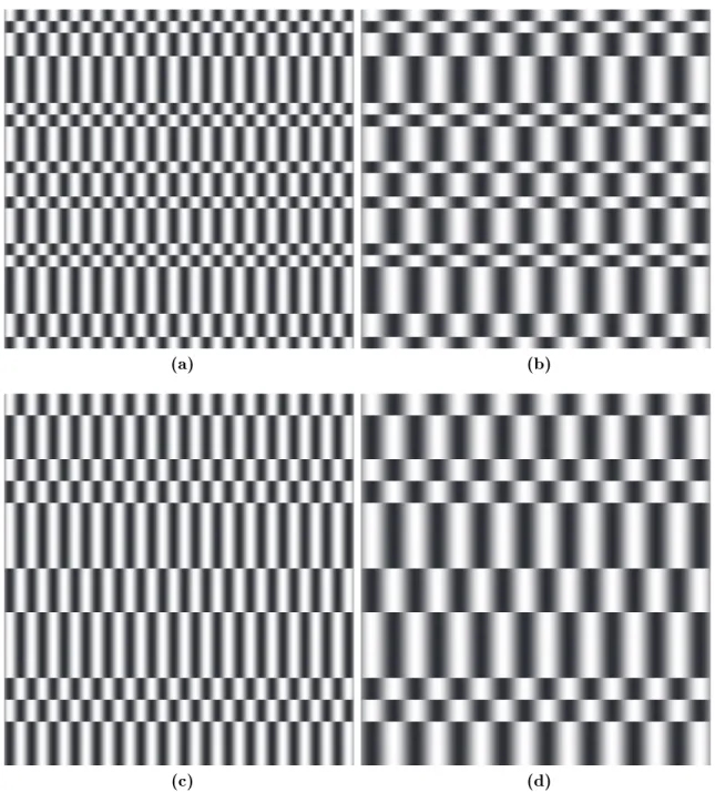
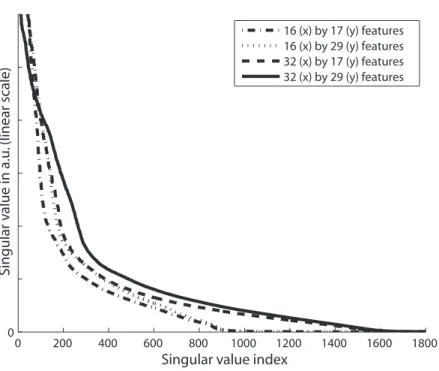
Figure 2.7 shows new aperture designs that have sinusoidal dependence on the horizontal (x) axis and a shift code in the vertical (y) axis using a quadratic residue code. The aperture resolution (number of code features) was varied separately in each direction to illustrate the scaling of the singular value spectrum, shown in Figure 2.8. Measurements were numerically simulated over a 100 mm×100 mm area and 96×96 samples. The object was represented by
(a) (b)
(c) (d)
Figure 2.7: Coded apertures based on a sinusoid inx (horizontal) and a quadratic residue in y (vertical). The number of code features in each direction (x, y) are (a) 32×29, (b)
0 200 400 600 800 1000 1200 1400 1600 1800 0
2 4 6 8 10
12x 10
6
16 (x) by 17 (y) features 16 (x) by 29 (y) features 32 (x) by 17 (y) features 32 (x) by 29 (y) features
Singular value index
Si
n
gu
la
r v
alue
in
a.u
. (linea
r sc
ale)
Figure 2.8: Singular value spectra for each of the coded apertures in Fig. 2.7.
Figure 2.9: Coded aperture with resolution 32×29 based on uniform random values in
[0,1].
0 500 1000 1500 2000 2500
0 2 4 6 8 10 12x 10
6
Harmonic (x) MURA (y) Random
Singular value index
Si
n
gu
la
r v
alue
in
a.u
. (linea
r sc
ale)
Figure 2.10: Singular value spectra for the proposed code and a random code.
The coded aperture with 32×29 features was compared with a similar random code drawn
CAXSI systems using the two codes are shown in Figure 2.10. For the rst 620 singular values the new Harmonic-MURA code outperforms the random code but then a crossover occurs and the random code produces a more slowly decaying spectrum. One can expect that the random aperture will perform worse in a noisy environment where a limited number of singular vectors are measurable.
2.5 Scalability of imaging techniques
This section compares CAXSI with Radon imaging and selected volume tomography (SVT) for 2D tomography under the constraint of xed radiation dose delivered to the object. The singular values for each technique scale with the resolution of the desired image, where it is assumed the number of measurements M equals the number of object coecients. Radon imaging is a method of transmission tomography where the measurements are line integrals of the target's density. Radon imaging requires multiple exposures for each tomographic image. The singular values of the 2D Radon transform are λm =
p
4π/(m+ 1) [64], with
each value having a degeneracy of m + 1. The Radon transform therefore yields typical
singular values proportional to 1/M1/4. Letting N be the number of reconstructed pixels in each object dimension, M = N2 so the singular values are of magnitude 1/√N. A pencil beam scanned over a plane produces N subspaces each with N singular values proportional to 1/√N. For the Radon system to deliver the same dose as the scanned pencil beam, the source must be N times dimmer during Radon's N exposures. The eective scaling is then
1/N3/2 for Radon and1/√N for pencil beam CAXSI. Appendix B shows that the singular values scale like 1/N for fan beam CAXSI, and since this is a snapshot technique the dose is comparable to the scanned pencil beam.
a fan beam since these are the fractions of the total number of voxels contributing to each measurement.
Table 2.1 summarizes the scaling laws for 1D and 2D imaging using pencil and fan beam CAXSI, Radon imaging, and SVT. In each case the singular values are scaled so the maximum singular value corresponding to the constant singular vector is 1. Both pencil and fan beam CAXSI show improvement over other methods for 1D and 2D imaging. In addition, pencil beam CAXSI enables independent reconstruction of each ray, whereas planar Radon imaging multiplexes points over a plane. Independent reconstruction of each 1D subspace using pencil beam CAXSI enables spot tomography, where a single pencil beam illuminates a region of interest, eliminating unnecessary doses to neighboring regions.
Image dimension Pencil Fan Radon SVT
1D √1
N -
-1
N
2D √1
N
1
N
1
N3/2
1
N2
Table 2.1: Scaling of dose-constrained singular values for pencil beam CAXSI, fan beam CAXSI, Radon imaging, and selected volume tomography (SVT). In each case the singular values are scaled so that the maximum is 1.
These results assume equal photon eciency for scatter and transmission imaging. In practice, the scatter systems will include an additional factor for the fraction of the total scatter signal detected, and the ratio of scattered to transmitted photons for the object of interest. These eects should be studied carefully for particular imaging applications.
2.6 Summary
CHAPTER 3: PENCIL BEAM CAXSI
(Adapted from previously published work [31])
3.1 Background
This chapter describes a pencil beam x-ray system demonstrating coded aperture x-ray scatter imaging (CAXSI). In the previous chapter, sinusoid codes were shown to provide range resolution for pencil beam tomography. These ideas inspired the following experiment which demonstrates snapshot 1D tomography using a periodic coded aperture, while also measuring the coherent scattering density of the object at each point in the beam. In the language of Chapter 1, this corresponds to the transformation F(z, q) → G(x, y), where
F is the unknown scattering density and G(x, y) is the measured irradiance image. This is
closely related to the anisotropic systemF (z, θ)→G(x, y)from the last chapter, and would
be identical to it for the case of a purely monochromatic beam. In the following, coherent scatter imaging is achieved with angle dispersive measurements and a poly-energetic x-ray source.
CSCT uses a series of images recorded at multiple angles to estimate an object's coherent scatter properties. Another approach to scatter tomography is energy-dispersive x-ray diraction tomography (EXDT) [68], which scans an object voxel-by-voxel using collimators and provides an eectively isomorphic mapping between the object voxels and the measure-ments. EXDT was originally demonstrated with an x-ray tube and then with a synchrotron source [69]. It has been used to probe polymer and bone surfaces [65], to reduce the false alarm rate of luggage scanners in airline security [23], and to probe mineral content in thick cement samples [24].
Figure 3.1: Basic pencil beam coded aperture x-ray tomography system.
The goal of this chapter is to experimentally demonstrate pencil beam CAXSI by re-covering the momentum transfer prole of a scattering object at each point along the beam using a single irradiance image. The experimental system is depicted in Figure 3.1, including a 2D irradiance detector array perpendicular to the beam and a coded aperture between the object and detector to modulate the scattered radiation. To obtain a volumetric scatter image, the pencil beam could be scanned over a 3D object with estimation performed for each transverse position.
3.2 Forward model
In the pencil beam system depicted in Figure 3.1 the x-ray source is ltered by a pinhole to produce a pencil beam propagating along thezaxis, which for simplicity is assumed innitely narrow. The scattering object is placed between the primary and secondary apertures so that it is penetrated by the beam. The primary beam is stopped by the secondary mask to prevent it from ooding the detector image. Scattered x-rays diverge from the main beam to strike the aperture, where they are either absorbed or transmitted to the detector plane. Each pixel in the detector array receives scattered power from multiple points along the beam, and the structure of this multiplexing is controlled by the aperture code.
As discussed in Section 1.2.1 of Chapter 1, upon coherent scattering an x-ray photon changes its momentum by q= pf −pi, where pi is the incident momentum and pf is the
nal momentum. The coherent scattering condition is|pf|=|pi|, from which follows Bragg's
law q = 2cE sin θ2, where q = |q|, E is the x-ray energy, and θ is the scattering angle as shown in Figure 3.1.
The scattering densityF(z, q)is the probability that an incident photon scatters at beam
location z with momentum transfer q. This model only depends on the magnitude of the momentum transfer and not its direction, so it applies to liquids, ne powders (as in this experiment), and amorphous compounds. In the absence of a coded aperture, scattering at angle θ from position z produces an irradiance at radius ρ on the detector proportional to 1/(z2+ρ2). The coded aperture is modeled by the transmission function T(ρ, φ) in the plane z = d, where (ρ, φ) are the polar radius and angle relative to the beam. To within
some proportionality constant, the total irradiance at the detector point (ρ, φ) is
G(ρ, φ) =
dz
1
z2+ρ2
T
ρ
1−d
z
, φ
dq F(z, q)P
E = zqc
ρ
, (3.1)
P(E)is the power spectral density of the beam, assumed independent ofz so that the linear model applies. Equation (3.1) is the forward model for this pencil beam system, and consists of integrals of the scattering density overz and q. The argumentρ(1−d/z)to the
aperture transmittance T is the intersecting radius for the scattered ray connecting scatter point z and measurement radiusρ in the detector plane
In contrast with previous studies of coded aperture imaging that emphasize shift codes based on their properties under translation [56], range imaging requires scale codes that are maximally distinguishable under magnication. As discussed in Chapter 2, equation (3.1) is a scale transformation of the aperture code T(ρ, φ) which depends on the scatter
position z. The projected image of the aperture code is magnied by z/(z −d). One can
disambiguate scatter points at dierent values of z by applying aperture codes which are orthogonal under changes in scale (i. e. magnication). Sinusoid codes (e.g. T(ρ) = cos(ρ))
have this property. To also disambiguate q the code must also vary as a function of φ. As binary codes are easily manufactured, we chose the square grid
T(ρ, φ) = 1 + sign (sin(ux))
2 , (3.2)
whereu is the spatial frequency and x is a Cartesian coordinate in the ρ, φplane. Equation (3.2) describes a binary version of the sinusoid, where the transmittance values lie between zero and one in accordance with incoherent imaging. An x-ray projection of the correspond-ing physical aperture is shown in Figure 3.3, which consisted of periodic slits drilled in to a lead plate. This x-ray projection image was used for T instead of (3.2) for better model accuracy.
The continuous forward model (3.1) is discretized by expanding the scattering density over compact voxel functions in the coordinates z and q. For this purpose we use the function rect(x) which is equal to unity for |x| < 1/2 and zero everywhere else. The
![Figure 2.9: Coded aperture with resolution 32×29 based on uniform random values in [0, 1]](https://thumb-us.123doks.com/thumbv2/123dok_us/8322246.2206075/50.918.302.618.104.434/figure-coded-aperture-resolution-based-uniform-random-values.webp)
