PARTISAN POLYGONS: GEOGRAPHIC COMPACTNESS AND EFFICIENT GERRYMANDERS
John A. Curiel
A thesis submitted to the faculty of the University of North Carolina at Chapel Hill in partial fulfillment of the requirements for the degree of Master of Arts in the Department of Political Science, Concentration in Comparative Politics .
Chapel Hill 2016
ABSTRACT
JOHN A. CURIEL: PARTISAN POLYGONS: GEOGRAPHIC COMPACTNESS AND EFFICIENT GERRYMANDERS
(Under the direction of Thomas Carsey.)
TABLE OF CONTENTS
LIST OF TABLES . . . v
LIST OF FIGURES . . . vi
The Forgotten Half of Gerrymandering . . . 3
Compactness and Partisan Bias . . . 5
Data and Methods . . . 16
Results . . . 23
Discussion and Conclusion . . . 33
Appendix A . . . 36
Appendix B . . . 37
Appendix C . . . 42
LIST OF TABLES
Table
1 District Compactness Ranges Given Unified Party Redistricting . . . 7
2 Democratic Presidential Vote Share State - District Deviance . . . 25
3 District Compactness Preferences OLS Regression . . . 29
4 Continuous Variables for District-State PVS Deviance Table . . . 36
5 Categorical Variables . . . 36
6 Continuous Variables from Table 2 . . . 37
7 Extended Models of Table 1 and Robustness Checks . . . 42
8 Second Analysis Robustness Checks . . . 43
9 Principle Component Factor Analysis of Compactness Measurements . . . 43
LIST OF FIGURES
Figure
1 Non-Compact versus Compact Districts . . . 4
2 Gerrymanders of Cities . . . 9
3 Convex-Hull Transformation of NC-12, 2011 . . . 18
4 Convex-Hull Compactness Distribution . . . 23
INTRODUCTION
Since America’s conception, the nation wrestled with the undemocratic consequences arising from the utilization of districts as jurisdictions for U.S. Representatives. True re-publican governments require citizens to choose their representatives. However, the ability of House members to influence where district lines are drawn allows them to choose their voters. The ability to redistrict is the power to manipulate the public in pursuit of more power.
America’s storied history to cope with the manipulation of political boundaries by office holders led to the seemingly intuitive utilization of compact districts. While numerous def-initions exist for compactness, the common understanding is that an ideal compact district resembles a non-disperse regular polygon. Compactness appeals to a sense of democratic aesthetics; a non-compact district hints deviations from a neutral district in order to benefit an incumbent or party. Justice Anthony Kennedy inDavis v. Bandemer (1986) went so far as to argue that compactness is an “objective factor” which determines whether a district is gerrymandered.1 The U.S. Supreme Court in part adopted Justice Kennedy’s affinity for compactness as a useful criterion in determining gerrymanders inDavis v. Bandemer(1986) 478 U.S. (at 173) (Niemi, Grofman, Carlucci & Hofeller 1990). The arguments of redis-tricting reformers and the Supreme Court over time influenced eighteen states to implement compactness as a primary criteria in redistricting congressional districts (Levitt 2010).
Despite the perception of compactness as an objective non-partisan factor in redistrict-ing, I argue that this belief is misinformed. In reality, compactness has an anti-Democratic bias even while the courts and redistricting reformers draw compact districts arising from the perception that it is truly non-partisan and objective.
The biased effect of compactness arises from the high concentration of Democrats in
cities. Democratic redistricters cannot draw districts that extends their voting blocs across the state. However, the Republican redistricters face no such constraint when redistricting for their party’s advantage; they can even draw compact district maps and still gerrymander states in their favor to secure large and stable congressional majorities. At the same time, state courts and independent commissions without as strong a partisan motivation, coupled with some to appear legitimate and unbiased, prefer to draw compact districts as an end in and of itself while ignorant of the partisan bias of district compactness.
What leads the divergence in partisan handling of compactness to be of practical in-terest arises in regards to the increasing role of courts and independent commissions in redistricting. Courts and commissions under the belief that compactness constrains parti-san gerrymanders will be more prone to draw compact districts as a means to redistrict in what they believe to be a non-partisan fashion. I posit that the partisan constraint model as applied to the less partisan courts and independent commissions leads to increased consid-eration of compactness as a non-partisan principle. Partisan constrained bodies give weight to other concerns, like the law and governmental efficacy, while also trying to advance their partisan interests (McKenzie 2012, Baum 2006). They accept the arguments presented by legal scholars of compactness as a constraint on gerrymandering.
The Forgotten Half of Gerrymandering
The United States Supreme Court revolutionized congressional redistricting post-Wesberry v. Sanders(1964) by mandating the “one person, one vote” principle. Equal populations within districts is utilized as the primary criteria by which district maps are arbitrated, though the Court will permit greater deviation from this principle if Traditional District-ing Principles (TDPs) are at stake. The TDP of interest for this research is geographic compactness.
Geographic principles tend to be granted less importance than outcome criteria in re-districting debates and research. Computational limitations greatly limited compactness research as GIS software up until the 1990s might take days to process the necessary data (Niemi et al. 1990). Despite the limitations in previous research, geographic compactness is a fundamental component of redistricting. The goal of geographic compactness require-ments is to prevent parties from choosing individual voters through the utilization of con-torted district boundary lines (Polsby & Popper 1991). Gerrymandering at its core is the violation of some geographic standard which dilutes the representation of a state’s citizenry. Geographic districting principles act as a proxy for community representation, and cru-cially, cohesion (Levitt 2010) and signals when redistricters go out of their way to benefit a party or incumbent (Altman, Amos, McDonald & Smith March 22, 2015). A snake-like district may prevent the voters in a district from interacting with each other. Compactness requirements attempt to place people who commonly interact with each other due to geo-graphic proximity into the same district, which in turn leads to a sense of community in the district (Engstrom 2005, Forgette, Garner & Winkle 2009, Bowen 2014, Niemi et al. 1990). Judges across the nation perceive non-compact districts as an expressive harm to Amer-ican republAmer-ican governance (Pildes & Niemi 1993). However, despite the acceptance of compactness as a TDP for these reasons, no state court has yet to incorporate quantita-tive scores of compactness in their decisions and overwhelmingly rely on visual inspection (Engstrom 2002, 65-66).
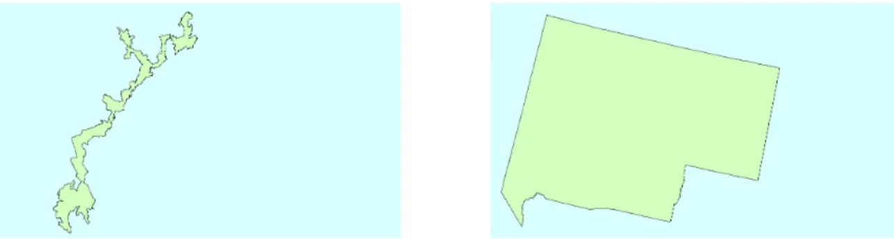
with non-contorted boundaries and less geographic dispersion are more compact (Polsby & Popper 1991, Reock 1961, Niemi et al. 1990). Thus, a compact district would tend to be a circle or regular polygon as opposed to a long and snaking district. An example of the different ends of the compactness spectrum can be seen in figure 1.
Fig. 1:Non-Compact versus Compact Districts
Map created using U.S. Census data.
North Carolina’s 12th Congressional District (left) and Nevada’s 2nd Congressional District (right), 113th Congress
No matter the definition, compactness always decreases as the perimeter of a district increases at a rate that outpaces its area. As seen in Figure 1 with North Carolina’s twelfth district, the many appendages and corridors increase the dispersion of the district, which lowers compactness. Nevada’s second district is considered compact; almost a square, and lacking notable contortions.
Whether compactness exerts a substantive impact on the boundaries of districts and po-litical action is not clear. Altman (1998) examines several TDPs and their use over Amer-ica’s redistricting history and found a drop in compactness followingBaker v. Carr (1962). Several states adopted compactness as a means to prevent political manipulation of dis-tricts prior to 1860 (Kromkowski 2002, 352–351). These early state constitutions, such as Kentucky’s, stated that districts should be drawn into “squares which are contiguous.”2 To date the evidence is weak that compactness as a TDP restrains partisan gerrymander-ing, or has other positive effects. Engstrom (2005) found a complete lack of evidence between more compact districts and voter turnout, highlighting that compact districts do not lead to increased political participation or trust in government. Furthermore, Forgette,
Garner & Winkle (2009) discerned no connection between compactness requirements and competition in state legislative races, while Altman found no relationship between national compactness requirements from 1901-1929 and the compactness of districts. Only Bowen (2014) discerns a positive effect of compactness requirements, finding that increased com-pactness may increase constituent satisfaction with their representative.
Evidence thus far suggests that compactness poses a minor obstacle to gerrymanders at best. This does not mean compactness has no political impact; rather there is a grow-ing concern that TDPs are not politically neutral. Since Democratic voters geographically concentrate themselves into cities (Bishop 2008), it is posited that Democrats suffer de-creased representation when districts are drawn to be more compact (Taylor & Gudgin 1976, Erikson 1972, Erikson 2002, Lowenstein & Steinberg 1985). For example, a Democratic attempt to capture more seats would require pairing urban areas with stretches of non-urban areas. Therefore, a Democratic attempt at gerrymandering would necessitate non-compact districts and raise greater suspicions of gerrymandering than such attempts carried out by Republicans. Chen & Rodden (2013) simulate redistricting to demonstrate that Democrats capture significantly fewer House seats when compactness is maximized and claim that the effect amounts to an “unintentional gerrymander.” It is not clear that party preferences of compactness arise from ignorance of its effects.
Compactness and Partisan Bias
I argue that the foundation of partisan bias in compactness arises from the non-uniform and clustered distribution of Democratic voters. Homogeneous concentrations of Democrats living in urban areas violates basic assumptions by reformers in favor of compact districts. These clustered Democrats go on to permit parties interested in capturing more seats to use compactness in different ways in their pursuit of partisan gerrymanders.
sam-ple of all interests in the state, which is the case with at-large districts. Functional districts represent particularized group interests (209–10). Compact districts in theory constrains functional partisan districts and limits boundary contortions (Polsby & Popper 1991, Niemi et al. 1990). When redistricters contort boundaries, they presumably deviate from a normal polygon shaped randomized district in order to benefit themselves via a functional district. While redistricters might still position districts for partisan gain, randomized districts are far more representative. Assuming a random distribution of voters, the placement of regular polygon shaped districts would capture on average a representative subset of voters.
However, regular compact districts will not symmetrically constrain partisan gerryman-dering given that the distribution of partisans is not random. Polsby & Popper (1991, 336–7) argued a non-random partisan distribution as unlikely. It is now well established that Democrats cluster into urban areas while Republicans live in suburban and rural areas (Bishop 2008, Chen & Rodden 2013, Taylor & Gudgin 1976). Given that Democrats dis-proportionately draw on support from urban centers, they contort district lines in order to achieve any party gain. Should Democrats draw compact districts, they will win only urban districts and leave the rest of the state to Republicans.
Given that Democrats primarily live in cities, the same redistricting strategies practiced by different parties will result in fundamentally different district designs and compactness. Redistricting by the state legislature predominantly takes the form of either incumbent ger-rymanders, which secure easy reelections for incumbents, or partisan gerger-rymanders, which maximizes stable majorities for the party redistricting. The two strategies are at opposite sides of a continuum; the more partisans given to an individual incumbent, the less parti-san voters available to the party at large to secure more congressional seats. From a party perspective, incumbent gerrymanders are innately inefficient. An efficient partisan gerry-mander is one where a party maximizes the number of stable seats for the smallest possible marginal vote in every district (Engstrom & Kernell 2005, Cain 1985).
voters will loyally turnout. How certain a party is of their turnout constrains their design of districts across the state. A party certain of 100 percent turnout across the state with a statewide partisan advantage would be able to construct the most efficient gerrymanders and win each district by one vote. When redistricting, a party would therefore engage in “cracking” and create marginal districts across the state in their favor and diluting sizable voting minorities of the opposing party (Cain 1985).
When parties cannot increase their partisan balance in a district given their insufficient number of voters in a state or uncertainty as to loyal turnout, they will have to engage in their second best strategy for efficiency, known as packing. Under a packing strategy, a party will pack voters of the opposing party into a minimal number of districts. These packed districts ideally would be comprised entirely of the opposing party’s voters. This leaves the rest of the state with districts winnable for the party in charge of redistricting (Engstrom 2013, 28–9). Incumbents, especially minority party members, will enjoy greater security in a packing plan as opposed to a cracking plan given the greater concentration of partisans. However, a packing plan will still result in more competitive seats given that the intent is not to grant incumbents complete security (Gelman & King 1994b, Cox & Katz 2002).
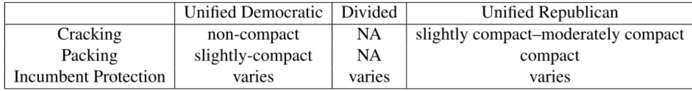
Were partisans uniformly and randomly distributed across the state, so that urban voters were no more likely to be Democratic relative to rural or suburban voters, district compact-ness would be dependent on how much a party desires districts to approximate the state as a whole. However, given that Democrats are clustered, district compactness depends on the party in charge of redistricting and the tactic chosen, as elaborated in Table 1.
Table 1:District Compactness Ranges Given Unified Party Redistricting
Unified Democratic Divided Unified Republican
Cracking non-compact NA slightly compact–moderately compact
Packing slightly-compact NA compact
Incumbent Protection varies varies varies
Of all the redistricting possibilities, the least compact should be Democratic cracking plans. This follows given that the clustered nature of Democratic voters will require stretched out districts radiating from cities should Democratic leaders seek to increase their number of seats. Packing plans for Democrats should only be slightly compact at best; while a couple districts should consist of packed Republican rural and suburban areas, Democrats will still have to draw districts radiating from cities in order to win more seats. Republican unified governments would be able to crack Democratic enclaves in a comparatively more compact manner as they can attach their large blocs of non-urban voters to urban areas via appendages small relative to the entire size of the district.
Figure 2 demonstrates Democratic and Republican cracking plans made possible due to the sorting of Democrats into cities. In the state of Illinois, Democrats redistricted and needed to spread their support in Chicago to the rest of the state in order to win more congressional seats. Therefore, they drew the districts overlaying Chicago to pair urban Democrats with suburban Republicans, which diluted the Republican vote. Republicans in Texas, meanwhile, cracked the city of Austin. Of the ten districts that overlay Austin, eight are Republican and two are Democratic. The large Republican sections of the state effectively dilute the very liberal Austin area. The districts may not be as compact as redistricting reformers would prefer, yet the districts are more compact in aggregate than a Democratic plan. The Republican districts further look somewhat like regular polygons. Were someone to simply judge gerrymanders based off of compactness alone, they would find the Democratic cracking scheme the offender.
The most compact of all redistricting plans will be Republican packing plans, as these will pack most Democratic urban voters into condense non-disperse areas while leaving the rest of the state free to be redistricted into compact districts which act as somewhat biased microcosms of the state in regards to partisan balance.3 Incumbent protection gerrymanders should depend primarily on districts’ shapes from the previous redistricting
3For example, the original 1812 gerrymander in Massachusetts packed eastern Federalists into a single
Fig. 2:Gerrymanders of Cities
Map created using U.S. Census data.
The 2010 cycle districts of Illinois overlaying Chicago (top) radiate outward; congressional districts overlaying Austin, Texas (bottom) consist of large areas that consists of only small parts of Austin.
cycle and be most common in divided governments.
partisan gerrymanders. Thus, an anti-Democratic and pro-Republican bias exists when compactness is held as a strict standard. However, whether partisan gerrymanders take place rests upon the strength of a party to push their map through a state’s government.
Party Cartels and Efficient Gerrymanders
I theorize that state parties in legislatures redistrict as cartels interested in maximizing party power. The party cartel in power makes the redistricting decisions regarding com-pactness and can thus influence who can win congressional seats.
Party cartels control state institutional power and attain collective goods to benefit the party. Cox & McCubbins (1993) argue that parties, via strong leaders, seek to maximize collective goods for the party’s members by usurping the power of government branches and jurisdictions. Party leaders further whip and coerce members into following the party line for their party’s own collective benefit. In line with Cox & Katz (2002), I argue redistricting is a collective good that party leaders use to advance their party’s power in government. Parties as political organizations benefit from more control over government, fostered by increasing their number of secure congressional seats. The means to maximize the number of representatives in large part relies on the number of efficiently gerrymandered districts in favor of the party (Engstrom & Kernell 2005). To draw districts on a statewide scale to the benefit of the party requires that individual districts do not contain too large a percentage of a party’s statewide voter base; parties cannot afford to allocate most of their partisan voters to a few representatives in completely safe seats. As a result, partisan gerrymanders lead to slightly more competitive seats than incumbent protecting gerrymanders.
possibility of individual cheating and prevent collective action dilemmas.
I argue that parties and their leaders concern themselves with geographic compactness given its role in achieving efficient partisan gerrymanders, which increase party power. Compactness arises as a component of gerrymandering given that Democrats are concen-trated in cities across states, which biases congressional maps towards the Republican Party when compactness is increased. Democratic leaders must violate compactness in order to efficiently allocate their supporters whereas Republicans do not.
The duty of party leaders is to adopt the best tactic in achieving an efficient partisan gerrymander. Leaders can take advantage of the Democrat-Republican partisan balance in a state, along with the distribution of partisans. A party with a statewide majority initiates an efficient gerrymander by drawing districts to resemble a microcosm of the state partisan balance, which takes advantage of their greater share of voters (Cox & Katz 1999, 821). The party then goes on to increase their ratio of partisans in necessary districts in order to increase the security of a district to a satisfactory level.
Parties need to carefully consider how responsive they wish to draw a given state’s congressional map. If a party holds a 70-30 statewide vote advantage, they should be able to hypothetically draw each district as a microcosm of the state, ensuring a safe margin of victory. However, closer margins lead to greater risk. As Engstrom & Kernell caution, the partisan redistricting during the Gilded Age led to constant shifts in party control of state legislative and congressional majorities. This in turn led to approximately half of all congressional races at the time to be competitive (Carson, Engstrom & Roberts 2007). While a party would like to win as many seats as possible, they would also prefer stable majorities. It does the party no good should they win all of the congressional seats one election only to lose the entire delegation in the next.
this might amount to the state party agreeing to use more state resources to advertise and support the congressional representative’s next campaign. The end result is a unified party effort to secure the largest number of secure congressional seats as possible.
Therefore, unified party governments empower leaders to pursue their ideal partisan ger-rymandering strategies. The resulting compactness and shapes of districts in turn greatly differ between parties due to how party leaders take advantage of clustered Democratic voters. Clustered Democratic voters constrain how compact Democratic leaders can de-sign districts. Democratic redistricting will necessitate disperse districts. Thus, Democratic leaders prefer non-compact districts. Republicans in turn do not perceive compactness as a threat to their stable congressional majorities and can even benefit from increased com-pactness in attaining more seats. Therefore, the ability for Democrats to engage in efficient gerrymanders lies in drawing non-compact districts. Meanwhile, Republicans can achieve efficient partisan gerrymanders via compact districts (compared to divided and Democratic unified governments). I therefore predict the following hypotheses:
Hypothesis 1: Unified Republican state governments will redraw congressional districts so as to increase the geographic compactness on average.
Hypothesis 2: Unified Democratic state governments will redraw congressional dis-tricts so as to decrease geographic compactness on average.
State Supreme Courts and Independent Commissions
Although party leaders use compactness for partisan collective gains, I argue that the non-legislative redistricters in the form of courts and independent commissions also utilize compactness, buying into the belief of compactness as an objective and non-partisan crite-rion. Compactness as a gerrymandering constraint dates at least to the 1840s (Kromkowski 2002). Legal scholars spearheaded the move to raise compactness as a key principle for redistricting (Engstrom 2005, Stern 1974) and 18 states now mandate compact congres-sional districts (Levitt 2010). The U.S. Supreme Court cited compactness as a “useful criterion” for gerrymandering cases inDavis v. Bandemer478 U.S. (at 173) (1986) (Niemi et al. 1990). InMiller v. Johnson(1995) the Supreme Court required redistricters demon-strate adherence to compactness and several other TDPs in drawing majority-minority dis-tricts.4 The Supreme Court reasoned that non-compact districts produced “expressive harm” whereby the explicitly gerrymandered districts decrease trust in government and alienate voters (Pildes & Niemi 1993).
Following the partisan constraint model, bounded partisans primarily consist of judges and politician commissioners. Bounded partisans need to give concern to such non-partisan principles at the expense of any non-partisan preferences they may have (McKenzie 2012, Baum 2006, Braman & Nelson 2007). They are not neutral arbiters, though they are not the unfettered partisans akin to state legislators. There is some expectation of judges, commissioners and bureaucrats to respond to the interests of the people as opposed to merely partisan interests. Faith in government officials to act in the interests of the peo-ple is known as democratic efficacy. Citizens low in efficacy perceive the government as unresponsive to their interests, eventually become alienated and resent government officials (Morrell 2005). Given that the partisan constraint model expects bounded partisans to give greater weight to upholding efficacy, I expect courts and commissions to favor increasing compactness in deference to democratic efficacy. State redistricting bodies less moved by party interests should be expected to pursue compactness for its own sake.
The partisan constraint theory would predict courts least influenced by partisan con-cerns to give greater weight to efficacy and therefore compactness. Constrained partisans are those evaluated for upholding the law and non-partisan principles. These constrained partisans further lack as great an individual incentive to pursue party interests due to their inability to campaign on a partisan platform. I apply the partisan constraint model to state supreme court justices in particular given that state supreme courts are the primary bod-ies responsible for redistricting and upholding TDPs should the legislature fail to pass a map5 (Levitt & McDonald 2007, Engstrom 2002). Of the five state justice selection types, the two least partisan are non-partisan and retention elections. These systems institution-alize positive and negative incentives to uphold non-partisanship. Overly partisan deci-sions attract quality partisan challengers, which may cost a sitting justice their seat (Hall & Bonneau 2006). Some state governments even send “report cards” to voters on the voting records and backgrounds of incumbent justices for retention and non-partisan elections.6 State parties face obstacles to fund-raising in these elections as well (Bonneau, Hall & Streb 2011).
Courts are substantial threats to state legislatures during redistricting. The state supreme court redistricts should technical map flaws arise or the legislature fail to redistrict. Courts may adopt a submitted map or draw one (Levitt & McDonald 2007). While parties might expect partisan selected courts to side with their proposal, non-partisan courts are more unpredictable. Given that non-partisan selected justices have less incentive to side with their party when the cost of efficacy is high, I predict the legislature to expect non-partisan courts to draw more compact maps compared to ideal legislative drawn plans. The legislature should preempt the court and address their concerns for efficacy, which leads to:
Hypothesis 3: The presence of a non-partisan or retention elected state supreme court in a state will increase the compactness of congressional districts relative to states with partisan selected justices.
5State supreme became the dominant arbitrators in redistricting followingGrowe v. Emison(1993) 507
U.S. 25, which told federal courts to defer to state supreme courts in redistricting cases (Engstrom 2002, 57).
The partisan constraint model also expects courts to consider the law in their decisions. Eighteen states require compact congressional districts. Yet given the importance that courts grant to partisanship on partisan issues (Caldarone, Canes-Wrones & Clark 2009), I do not expect legislatures to preemptively alter their redistricting strategies from compactness requirements alone. Non-partisan courts are another necessary condition. I expect non-partisan courts to be the body most willing to enforce compactness laws. State legislatures will predict the dual impact of a non-partisan court and compactness requirement and pre-empt the court, leading to a conditional hypothesis in the form of hypothesis 4:
Hypothesis 4: The presence of a non-partisan court with a compactness requirement will increase congressional district compactness in a given state.
State legislatures may attempt to preempt courts, though courts and commissions still redistrict. Courts and independent commissions are seen as less biased redistricters given their lack of personal electoral interests in redistricting (Levitt & McDonald 2007). The combined concern for efficacy and lesser partisan attachments leads to hypothesis five:
Hypothesis 5: Courts and independent commissions will draw more compact district maps than the state legislature.
Data and Methods
I test my expectations in a two part analysis. The first analysis links compactness to par-tisan efficient Republican gerrymanders, which is the necessary precondition before testing the hypotheses. The second analysis demonstrates consistent divergent preferences between parties, courts and independent commissions as elaborated in hypotheses one through five.
Each analysis measures a different dependent variable of interest. For the efficient ger-rymander test, the dependent variable is the absolute difference in district presidential vote share from the state average. The second analysis dependent variable is district compact-ness, which tests the different preferences over geographic compactness.
Establishing Republican Efficiency Bias
The efficient partisan gerrymander test determines whether compactness allocates the Republican voter more efficiently. The analysis examines congressional district level ab-solute deviation from the statewide presidential vote share.7 . A district with a smaller deviation from the statewide vote is closer to a microcosm of the state (Cox & Katz 1999, 850). The greater the absolute deviance from the statewide presidential vote, the safer the district is for an incumbent. A party interested in maximizing seat gain, which also wins the statewide presidential vote, would tend to desire less district deviation from the statewide partisan ratio. The larger the party’s statewide vote share margin, the more comfortably a party can make districts resemble the state. I found the average statewide Democratic pres-idential and district vote share by decade for each congressional district’s duration from the Database on Ideology, Money and Elections data set produced by Bonica (2013).8 5,911 observations existed for use from 1983–2011.9
7The most common duration is for ten years, following the normal decennial redistricting process.
How-ever, state legislature or courts may redistrict mid-decade, which leads to variations in the duration of districts
8The DIME data contains missing values for districts which states lost prior to the 2000 decennial
re-districting. The number of districts not present were few enough in number so as not to bias or impair the results
9When outliers that either have no deviation from the statewide vote or completely deviating districts are
The first analysis’s key independent variable is district compactness in Republican lean-ing states. If increased compactness leads to more efficient Republican gerrymanders, then compactness should decrease the presidential vote share difference between the state and district.10 Democratic leaning states should in turn see no or an opposite effect from in-creased compactness. Given this asymmetric effect, the variable of interest is an interaction between Republican leaning states and compactness. I code Republican leaning states as one where the Democratic presidential vote share is below 50 percent. Any state where this condition is present is coded as 1, and 0 otherwise.
I measure compactness using Convex-Hull dispersion area scores. Compactness is pri-marily measured via perimeter or dispersion scales (Bowen 2014, Niemi et al. 1990). I use Convex-Hull compactness as the best compromise measure. Convex-Hull scores com-pare the area of the congressional district to the smallest fitting convex polygon around the district. All compactness measures assume an ideal district shape. Compactness scores amount to a deviation of the actual district from the ideal shape, usually on a 0 – 1 or 0 – 100 scale. All compactness measurements parameterize the ideal shape and reflect penalties for boundary contortions (i.e. appendages, snaking districts). Convex-Hull scores grant flexi-bility by holding as ideal any non-concave polygon, which ends up moderately penalizing boundary contortions. Figure 3 demonstrates the transformation for for North Carolina’s District 12 from 2011.11
The method divides the area of the actual congressional district (AreaD) by the area of
are analyzed, the number drops to 971.
10District state deviation should drop regardless of which party redistricts. Statewide presidential vote share
should be a sufficient condition in which parties will greatly vary in their redistricting behavior, regardless of whether the tactic is to crack or pack. For example, a state with divided government should see the greatest deviation given that an incumbent protection gerrymander will result. If compactness follows the hypothesized effect, then these incumbent protecting districts should greatly vary in shape. In a Republican leaning state, the more compact a district, the less it should deviate from the statewide vote, even if the GOP is interested less in acquiring seats and more so in protecting incumbents. Should Democrats control redistricting in a GOP leaning state, as they did in the South prior to 1994, then we should expect Democrats to conduct extreme packing plans and create extreme deviation in districts from the statewide vote. Thus, the important variable is statewide presidential vote as opposed to party control for this analysis.
11The GIS tool used was minimum bounding geography, which requires a GIS license. The python script
Fig. 3:Convex-Hull Transformation of NC-12, 2011
Original NC12 (left), Convex-Hull (right)
the transformed smallest fitting convex polygon district (Areac) to produce the score.
CHscore= AreaD
AreaC
∗100 (1)
The Convex-Hull score is multiplied by 100 and produces a range of results where a zero is a district that approaches a perfect line while a score of 100 equates to a perfect convex polygon (Pildes & Niemi 1993). Since a Convex-Hull polygon is unique to each district’s convex points, the ideal shape varies for each district. The benefit is that Convex-Hull scores never hold districts to an unattainable standard. For example, Reock and Polsby-Popper scores both hold circles as the ideal shape. Given that state governments never draw circular districts, these result in low ceilings for compactness scores. A Convex-Hull dispersion score reports how much the district’s actual fills in the area of the convex ideal polygon. For example, NC-12 in 2011 had a Convex-Hull score of 34.78, which translates to NC-12 only filling in 34.78 percent of the smallest fitting convex polygon’s area, as seen in Figure 3. In 2013, NC-12 (as seen in Figure 1) dropped to a score of 24.98. This reflects a 9.8 percentage point decline in the area that the district covered compared to its ideal convex polygon. While Convex-Hull Scores tend to be higher than other compactness scores, they correlate with each other well and the rank ordering of districts by compactness is nearly identical (Niemi et al. 1990)12
12Most of the variance between scores arises from Convex-Hull penalties towards Hawaiian districts for
The data required to calculate compactness scores are Congressional District shapefiles. GIS shapefile data for congressional districts were gathered from the Digital Boundaries Congressional District UCLA data set from Lewis, DeVine, Pitcher & Martis, which is derived from the U.S. Census TIGERLINES shapefile data set13. I created a ArcGIS 10.3 python toolbox to compute the compactness measures.
I determined when district changes occurred by computing the Convex-Hull scores for every congressional district within a given shapefile from 1973–2013. I merged all of the compactness scores together and produced a dataset of all the congressional districts. I then created a compactness difference variable which subtracted the current congressional dis-trict’s compactness from its lagged value. Whenever a non-zero difference arose, a district was coded as having changed.14
I then interacted the Convex-Hull scores (on a 0–100 scale) with the dummy variable for a Republican leaning state.15 I ran an OLS regression model on the district level difference from the state Democratic presidential vote share, with the Republican leaning state district level compactness as the key independent variable. I use state and year fixed effects and control for the interactive variable components.16
Partisan and Institutional Compactness Preferences
The second analysis determines whether parties, courts and independent commissions exert different effects on compactness. The dependent variable is district compactness.17 I
13Maps and Data: TIGER/Line Shapefiles. 2013. United States Census Bureau. Retrieved from https:
//www.census.gov/geo/maps-data/data/tiger-line.html (accessed September 29, 2015)
14Only when a redistricting occurred was a district included in the analysis
15Republican leaning states are used as the key independent variable given that statewide presidential vote
share will cause whichever party in charge of redistricting to diverge in preferences and effects of com-pactness. Excluding government control also allows for more observations, though the model with unified government and less observations is included in the appendix.
16Fixed effects are used in order to more rigorously test the data given the fewer number of controls. This
also decreases the probability that any significant results are due to bias (Clark & Linzer 2015).
17District level compactness is used both to increase model efficiency and capture the within state variation
use a pooled time series approach for every non-at-large congressional district from 1983– 2013. The analysis uses panel OLS regression with robust clustered standard errors by state. Also included is a lagged dependent variable for district compactness from the last redistricting.
I measure unified Democratic and Republican state governments with dichotomous vari-ables found with the partisan balance data set by Klarner (2013). I code from 1983–2013 when both houses of the legislature and the governors office are controlled by the same party. The dichotomous variables are coded 1 when unified, and 0 otherwise, which makes divided and quasi-divided governments the reference group.
The institutional selection method for the state supreme courts were found in Book of the Statesand confirmed via the National Center for State Courts.18 From theBook of the States, each state is coded so that the judges selected via retention or non-partisan elections are categorized as non-partisan and coded as 1 in the Non-partisan Court variable, and 0 otherwise.
Districting bodies utilized in each state were determined using the dataset, ”All About Redistricting,” authored by Levitt (2015) for the 2001 and 2011 redistricting cycles. State constitutions and The Book of the States were researched to find the default redistricting bodies (predominately the state legislature). Following this, it was discerned whether courts or commissions intervened from The Legislative Coordinating Commission’s summaries on redistricting cases19 . I condensed the redistricter types into four categories: state legisla-tures, state politician commissions, non-partisan/independent commissions and courts.20
Maps drawn by state legislatures are those in which the entire body formally had a say in drawing the map. A politician commission is one where a subset of legislative leaders and
the courts. Further, mid-decade redistrictings occurred in some states for individual districts while leaving districts on the other side of the state unchanged. Analysis at the district level will not substantively change the results so long as state effects are included in the model. Thus, district level analysis offers the most insight and takes into account the specificities and complexities of redistricting.
18(Uppal 1981, Knoebel 1991, Wall 2001, Wall 2011, NCSC 2016)
19(Wattson, Wice & Jernigan 2015)
other elected officials draw the districts. I coded non-partisan commissions as drawing the lines if the proposal for a map arose from a non-legislative body with at least some commit-ment for non-partisanship. The final category, courts, includes federal, state supreme courts and lower courts. I code the court as the redistricting body when they have three or more maps to choose from or if they directly drew the lines themselves.21
I used the same sources in discerning which bodies drew the district lines to code state compactness requirements. I created a dichotomous variable for whether a compactness requirement was present in a state for a particular redistricting cycle.
Controls
For the second analysis I control for multiple variables, including the congressional dis-trict’s compactness in the previous cycle. Most states modify existing districts when redis-tricting (Levitt 2010), so I account for this with the lagged compactness of a congressional district.
I also account for state compactness. Niemi et al. (1990) go so far as to state that the relative geography of a state is so important as to make cross state comparisons impossible with the technology available at the time. I use the same method for district compactness to compute state Convex-Hull scores. Additionally controlled for are changes in congressional seats. A state’s districts will necessarily change boundaries with the addition or subtraction of a new district (Levitt 2010, Cox & Katz 2002). I add in a variable measuring the net gain or loss in congressional seats for a state per decade, which takes the value of an integer gain or loss in seats, ranging from negative five to seven.
A final substantive control is whether the Voting Rights Act pre-clearance section covers a state. A state under VRA pre-clearance needs U.S. Justice Department approval for any district modifications (Levitt 2010). Given that Voting Rights Act clearance in the past in part relied on perceived violations of compactness, I account for this possible bias. I created a categorical variable that accounts for whether a state was covered partially or completely
21The reason for the three congressional maps is that usually an option of two maps simply means that there
by the Voting Rights Act pre-clearance formula.22
For the OLS panel regression models I employ state robust clustered standard errors to account for any other extraneous state effects. I use RCSEs as more rigorous means than random effects to control for correlation among districts within a given state. Further, RCSEs do not unnecessarily eliminate the between state variation associated with fixed ef-fects. Therefore, state robust clustered standard errors offers the ideal compromise between efficiency and bias.23 However, I do not seek to give the impression that robust standard clustered errors are flawless; King & Roberts (2015) name two primary concerns with the over-reliance on robust clustered standard errors. The first is the potential problem with all statistical methods, where the stochastic veracity of the model. The second is the possible misspecification of the model if the differing control types diverge substantially from each other (160). Therefore, I also run the model with state random and fixed effects and report the results in the appendix.24 If all three models end up reporting similar results, then there should be much more confidence in the strength of the model. If the three models substantively diverge, it would then suggest that further work needs to be done in order to specify the model parameters (King & Roberts 2015).
In summary, the first analysis will go onto establish the necessary precondition that compactness is a variable of importance in creating efficient gerrymanders. The second analysis will build off the first and determine the different preferences unified party govern-ments and partisan constrained redistricting institutions have on compactness, as elaborated in hypotheses one through five.
22The fact that the Voting Rights Act pre-clearance section was repealed in 2013 impacted only those states
with continuing litigation well after the traditional deadlines passed and thus does not impact the results.
23Efficiency was not as much a problem for the first analysis given that there were over three times the
number of observations and that there were less control variables. For example, in the first analysis the impact of a state’s compactness is captured as part of the fixed effects. In the second analysis, state compactness is its own variable, added in order to determine the constraint that state compactness imposes on district compactness.
24The fixed effects should be expected to diverge from the state robust clustered standard errors model more
Results
The analysis starts off by testing the impact of compactness on the efficiency of Republi-can voters throughout a state. The test uses OLS regression with state and year fixed effects, with district-state presidential vote share deviation as the dependent variable. The key in-dependent variable is the interaction between district compactness and Republican leaning states. If compactness leads to partisan efficient gerrymanders in Republican leaning states (and Democrats in turn must draw non-compact districts to prevent GOP gains) then the coefficient should be negative, as a sign of less district-state deviance. Should a Republican efficiency bias exist as measured by the presidential vote share deviance, the results would replicate and support similar findings in the past (Chen & Rodden 2013) and establish the necessary condition in order to determine divergent preferences over compactness.
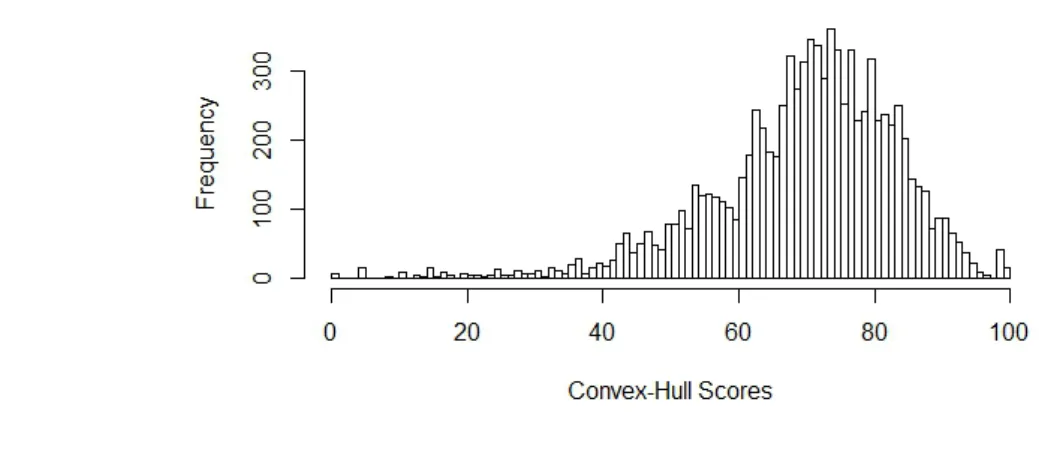
Congressional district compactness over the past 50 years provides a wide distribution of Convex-Hull scores, as seen in Figure 4. Convex-Hull scores center around a mean of 69.67 and a standard deviation of 13.77. As expected, Convex-Hull’s maximum score is 99 for Wyoming’s at-large district. The minimum value is 4.41 for Hawaii’s second district during the 1980s. This minimum value arises from one of Hawaii’s two districts dispersed across several islands. The nature of the data warrants caution for predictions near the upper and lower ends of the distribution.25
Fig. 4:Convex-Hull Compactness Distribution
25When these extreme values for presidential vote share deviance are excluded, the results do not
Compactness Effects on Redistricting Efficiency
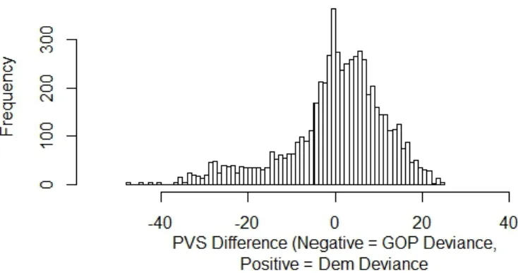
The first analysis tests the basis of the utility of compactness in achieving efficient Re-publican gerrymanders. As described previously, both packing and cracking plans should decrease the deviance in the district-statewide vote relative to incumbent protection plans. Further, Republican drawn packing and cracking plans should be more compact than the equivalent Democratic plans. The Republican Party with a majority of the statewide vote should seek to take advantage of their majority to attempt to win more seats overall, which results in increased compactness, as opposed to simply protecting incumbents. Figure 5 presents the distribution of district–state presidential vote share deviance. The negative end of the spectrum reflects districts winning less of the Democratic presidential vote share than the statewide average while the positive end reflects districts with a Democratic presidential vote share greater than the statewide average. The mean and median district–state differ-ence is zero. However, the distribution demonstrates enough variance in the district–state Democratic presidential vote share exists for analysis.
Fig. 5:Democratic Presidential Vote Share Non-Absolute State-District Difference
Scores on the negative side of the distribution are where the GOP share of the presidential vote share is greater than the statewide share while positive scores are those where the Democratic district share is greater than the statewide vote.
leaning states is a four-hundredths percentage point reduction in the district-state absolute deviance, all else equal. However, the interaction effect needs to be interpreted within the context of the Republican leaning state variable, which also attains significance. All else equal, Republican leaning states have districts where the average presidential vote share deviates by 3.91 percentage points; the effect is then moderated by district compactness in Republican leaning states and the relevant state and year fixed effects. District compactness alone does not reach significance.
Table 2:Democratic Presidential Vote Share State - District Deviance
Efficient Gerrymander
(Intercept) 5.6543∗∗∗
(1.1308)
District Compactness −0.0073
(0.0096)
GOP Leaning State 3.9072∗∗∗
(1.0224)
GOP State X District Compactness −0.0472∗∗∗
(0.0144)
Year Effects Yes
State Effects Yes
R2 0.1822
Adj. R2 0.1738
Num. obs. 5911
RMSE 7.0047
∗∗∗p <0.01,∗∗p <0.05,∗p <0.1
Unlike figure 4, the dependent variable is the absolute difference, which means that all scores are positive. The regressions are split so that Republican leaning states are those where the statewide presidential Democratic vote share is less then 50 percent while Democratic leaning ones are those above 50 percent. The number of observations will be greater than those in Table 3 given that observations are included wherever a district existed with its level of compactness for a presidential election. Fixed effects can be seen in the online appendix.
Table produced in R with the TexReg package (Leifeld 2013)
set.26 Texas and Florida are among the states which altered their districts by such an amount.
It is also possible to change multiple districts in order to alter a neighboring district. For example, if the Republican party saw a district that is split 50-50, they might increase the compactness of four neighboring districts by about 10 points each in order to change the evenly split district to 52-48 in their favor.
Despite the strict state and year fixed effect controls, the model suggests that the GOP leaning state effect leads to greater inefficiency from a Republican Party perspective. The means for the GOP to capture more seats then correlates with the level of compactness they are comfortable with for their districts. This in reality takes the effect of how many appendages and concave areas they are willing to add into districts in order to balance the security of their majorities relative to total seat gain. For example, the GOP in Florida during the 2011 redistricting chose to redistrict their congressional seats in a slight GOP leaning incumbency protection gerrymander where it was shown that the Republican Party created safe incumbent seats by adding in non-compact appendages into their district maps (Altman et al. March 22, 2015, 46). Thus, the analysis suggests that as confidence on the part of the GOP in their ability to win marginal elections, the more compact district maps can be drawn as part of a partisan gerrymander. However, it must be remembered that these are results on average; it would be foolish for any party to simply tell a GIS simulation to increase compactness and expect to win a stable and large congressional majority. These results do reinforce and replicate via a different means the findings of Chen & Rodden in finding a Republican bias in compactness, along with Altman et al. (March 22, 2015) regarding the method by which compactness is manipulated for partisan versus incumbency advantages.
It is possible that these initial results might be driven by outliers (i.e. districts that are perfect microcosms of the state and extremely deviant districts) or by party control of the redistricting process. I control for these both in Appendix B. Not only do the variables of interest retain significance, but the coefficient increases in size and even doubles in the
party control model. Therefore, these robustness checks suggest that compactness plays a role in impacting how districts deviate from the statewide vote, which goes onto influence party control of congress. If compactness were unbiased, as Polsby & Popper claim, then the variable for district compactness alone would reach significance and the interaction with GOP state would not. The results of table 2 and the appendix also make sense within his-torical context. For example, Democratic unified governments existed in the South in the early 1990s, yet governed states that started voting increasingly Republican at the presi-dential level. Democrats countered GOP gains via drawing some of the most non-compact districts in U.S. history, most notably in Texas, North Carolina, Louisiana and Georgia. Even non-majority-minority districts were non-compact (Monmonier 2001, Altman 1998). Democrats ultimately lost their hold of the South following the 1994 Gingrich Revolution, though their attempt to draw non-compact districts make sense within the context of the results in table 2 and GIS simulations by Chen & Rodden. Thus, impact of district com-pactness warrants further analysis into how parties and governmental institutions prefer district shapes.
Geographic Compactness Determinants
The initial support for compactness as a relevant variable for redistricting warrants an analysis regarding the determinants of compactness. The dependent variable for the second analysis is now district compactness. Given the suggested partisan effects of compactness on gerrymandering efficiency, parties should be expected to exert divergent compactness preferences. Of further interest is also whether courts and independent commissions per-ceive compactness as an objective non-partisan standard for redistricting. This second anal-ysis therefore tests hypotheses one through five.
Table 3 presents the results of the model for Convex-Hull compactness of congressional districts with robust standard clustered errors by state. The model explains 28.66 percent of the variance with 1,586 observations. The control for lagged compactness, which reaches significance, leads all of the coefficients to represent the marginal effect of an independent variable on change in compactness.
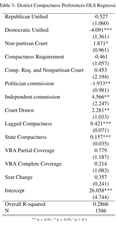
Table 3:District Compactness Preferences OLS Regression
Republican Unified -0.527
(1.060)
Democratic Unified -4.091***
(1.361)
Non-partisan Court 1.871*
(0.961) Compactness Requirement -0.461
(1.057) Comp. Req. and Nonpartisan Court 0.453
(2.194)
Politician commission -1.933**
(0.981) Independent commission 4.566**
(2.247)
Court Drawn 2.281**
(1.033)
Lagged Compactness 0.421***
(0.071)
State Compactness 0.157***
(0.035)
VRA Partial Coverage 0.779
(1.187)
VRA Complete Coverage 0.214
(1.083)
Seat Change 0.357
(0.241)
Intercept 26.058***
(4.744)
Overall R-squared 0.2866
N 1586
∗∗∗p <0.01,∗∗p <0.05,∗p <0.1
The number of observations is lower than table 1 given that only redistricting years are used.
initially simulated by Chen & Rodden (2013) exert real world political effects and lend credibility to the idea that compactness is a component of redistricting collective goods that party cartels consider.
that a legal challenge brings the congressional map before the state supreme court. Yet the results suggest that explicit compactness requirements do not impact compactness at all once controlling for the other factors.27 Therefore, hypothesis four does not receive sup-port. However, the coefficients are positive and significant for independent commissions and courts. Independent commission drawn districts are associated with an approximate 4.57 increase in compactness points. Court drawn maps on average increase compactness by approximately 2.28 points. These results follow hypothesis five and support the view that courts and independent commissions pursue compactness for its own sake. The re-sults also suggest that when Democratic governments cede redistricting power to courts or commissions, they can expect their preferred changes in compactness to be either halved or eliminated entirely. Overall, the partisan constraint model receives moderate support as courts and commissions appear to give greater weight to what is considered an objective TDP.
As for the controls, politician commissions, state compactness and lagged district com-pactness reach significance. The substantive effect for lagged comcom-pactness confirms the widely observed practice of modifying existing districts rather than starting from a blank map. State compactness significance confirms that district compactness is limited by the state’s compactness (Niemi et al. 1990, Pildes & Niemi 1993). The negative and signifi-cant coefficient for politician commissions might be related to the impact of more control by party leaders and merits future research. Neither VRA variable reaches significance. Changes in congressional seats reach significance, in line with Cox & Katz’s model.
The models with state random and fixed effects do not substantively differ, as demon-strated in Appendix B. None of the key explanatory variables fall from significance or change direction in the random effects model. The fixed effects model causes a drop in significance for those variables without enough within state variation (i.e. non-partisan courts) and drops from the model variables without any within state variation (i.e. state compactness and VRA coverage). However, significance still holds for Democratic
uni-27Even when the model variables are reduced, compactness requirements fail to reach significance. There
fied government, independent commissions and court drawn maps. The robustness checks therefore suggest that the model as specified does not experience substantive flaws and is a satisfactory starting point for this initial foray into preferences regarding compactness.
Geographic Effects of Significant Variables
To illustrate the general effect of the party and institutional variables on compactness, I take advantage of district compactness changes over time in order to demonstrate the aver-age effect. I provide figures demonstrating the effect for Democratic unified governments and independent commissions drawn maps (which are nearly exact polar opposites) as well as court drawn maps. A district is less compact when it contains more concave curves and dispersion relative to its ideal convex shape. The more disperse and concave a district, the more empty space that results when comparing the actual congressional district area to the ideal smallest fitting convex polygon. The maps include before and after versions of the coefficient effect along with a line connecting the convex points to clarify the ideal version of the shape.
Fig. 6:Compactness Effects of Democratic Unified Government and Commissions
Map created using U.S. Census data.
New York’s Fourth District. NY-4 in 2003 has a Convex-Hull score of 79.44. NY-4 in 2013 has a Convex-Hull score of 83.70. The difference is 4.26 points.
when a Democratic unified government or independent commission redistricts. A value of 4.26 falls within one standard error of the absolute value of the coefficient for both com-missions and Democratic governments. The Democratic effect would be a change from the 2013 district to the 2003 version, which would result in more concave spaces, appendages and decrease compactness overall. The independent commission effect would in turn be the change in compactness from the 2003 to 2013 district, the exact opposite of the Democratic unified government effect.
Both versions of the New York’s fourth district are above average compactness at scores of 79.44 and 83.70 respectively. The 2013 map increases compactness by reducing the severity of concave points relative to the latter version of the district. For example, the 2003 version’s eastern border is nearly completely cut in with concave points and noticeable appendages and this disappears for the most part in the 2013 version. The 2013 version increase compactness by transforming the district into a more square shaped district with a single moderate area of concavity on the western side. The southeastern district border now fits the convex ideal almost perfectly. Given the more convex area in the 2013 version of NY-4, independent commissions would prefer the latter version on average and Democratic unified governments would prefer the earlier 2003 version.
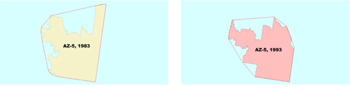
Fig. 7:Court Drawn Compactness Effects
Map created using U.S. Census data.
Arizona’s Fifth congressional district from 1983 to 1993. The district in the 1980s cycle had a Convex-Hull compactness of 73.18 compared to 75.63 in the 1990s, for a difference of 2.45 compactness points.
Average effects of direct court led redistricting is demonstrated in Figure 7. Arizona’s positive change of 2.45 represents the marginal improvement of court involvement.28 Both
28The change of 2.45 points falls within one standard error for the effect the presence of non-partisan courts
districts contain appendages which jet out from the core of the district. Yet the less compact 1983 version of AZ-5 contains a very large northern arm on the western side of the district, which is absent from the 1993 version. While the 1993 AZ-5 sacrifices some of its flat edges, the overall district becomes less disperse and marginally less concave.
It needs to be remembered that when looking at these geographic examples of gains in compactness that these are only a few of the infinite forms that compactness changes can result in. A nearly limitless array of districts exist for any given state at any given redistricting. What these figures exemplify are some of the ways in which redistricters change compactness. One might add on an arm to a relatively convex-polygon district and reduce compactness by several points or cut off appendages while modifying other district parts and still increase compactness. What these examples demonstrate is that the average expected changes in compactness can meaningfully change geographic boundaries. The addition or subtraction of appendages might easily concentrate opponents into a district and waste votes, efficiently separate the opposing party’s voters in an ideal efficient gerrymander or exclude an incumbent from their district. Geographic effects suggest that control and the nature of redistricting institutions warrants consideration and further analysis.
Discussion and Conclusion
Redistricting reformers seek to curb what they see as the worst excesses of partisanship in redistricting and an end to gerrymanders in general. Despite the seeming simplicity and justification of raising compactness as a principle to combat gerrymandering, the results found here suggest that compactness is susceptible to partisan bias, even while non-partisan actors prefer compact districts.
that state Democratic unified governments, which give rise to cartel control, prefer less com-pact districts. Republican leaning states with comcom-pact districts can permit more Republican congressional seat gains. Although Republican unified governments do not consistently pursue more compact districts, unified Democratic governments do consistently prefer less compact districts. Given that redistricting is a zero-sum game for power, Democrats most likely draw less compact districts to limit Republican gains while increasing their own. Therefore, unified Democratic governments which empower party leaders to force through their plans to efficiently gerrymander and thus co-opt state institutions for the collective good of the party.
Partisan redistricting is nothing out of the ordinary. Compactness at best appears to only act as one component of drawing responsive maps, dependent on contemporary geographic partisan sorting. What leads these results to be of note and possible concern is their percep-tion by legal scholars. Both courts and independent commissions apparently give weight to past U.S. Supreme Court rulings about TDPs and draw more compact districts in turn. This follows the idea that courts and commissions, even if comprised of partisan individuals, are constrained by other factors like efficacy. Even if compactness is not the central reason for striking down districts, it at least acts as a strong piece of evidence. As recent as February of 2016, U.S. Fourth Circuit Judge Roger L. Gregory struck down North Carolina’s first and twelfth congressional districts on the grounds that the “boundaries zig and zag to encircle African-American communities” and look “akin to a Rorschach inkblot.”29
Even the presence of non-partisan or retention elected justices appears to encourage the state legislature to draw more compact maps, while independent commissions exert a polar opposite preferences compared to Democratic unified governments. Increased com-pactness correlates marginally with more efficient gerrymanders at the district level, and the aggregate effect might offer the partisan edge in key competitive districts. These re-sults suggest that compactness cannot be viewed as some non-partisan objective principle. Should judges choose between two highly partisan maps on the basis of compactness alone,
29Anne Blythe, “Federal Court Invalidates Maps of Two NC Congressional Districts,Charlotte News and
Democrats would disproportionately suffer while Republicans could use compactness to their advantage in the court system. The Republican Party probably prefers the freedom to draw maps as they see fit given the unique conditions in each state at any given time. However, geographic compactness as a strict standard as mandated previous Congressional Apportionment Acts or as a judicial standard advocated by Polsby & Popper appears to fail to hold up as an objective criteria given the partisan bias and its demonstrated inability to increase voter turnout or political knowledge (Engstrom 2005).
These results in and of themselves do not suggest that compact districts are without worth; Democrats and Republican party leaders alike desire to control state institutions and goods in order to benefit themselves and craft policy in line with their ideologies. However, if true redistricting reform is to take place, then it must be acknowledged that compact-ness only impedes Democratic partisan gerrymanders. Some other criteria or system for redistricting is needed in order to equally constrain Republican partisan gerrymanders.
Appendix A
The following are the descriptive statistics from the first analysis in Table 1. The two continuous variables used for the first analysis in determining efficient gerrymanders are presented, the presidential vote share difference (dependent variable) and the district Convex-Hull compactness.
Table 4:Continuous Variables for District-State PVS Deviance Table
Variable Mean Median S.D. Min Max
PVS Difference 8.68 6.33 7.71 0 47.70
District Compactness 68.67 70.68 13.77 4.40 98.71 There are 5,911 observations from 1983–2011 where the presidential vote share was present for all non-at-large districts.
The Following are the descriptive statistics for categorical variables from both the first and second analyses in tables 1 and 2.
Table 5:Categorical Variables
Variable Yes No Percent
GOP Unified Govt 380 1,195 24.13%
Democratic Unified Govt 486 1,089 30.86%
Leg. Drawn 894 681 56.76%
Pol Com Drawn 124 1,451 7.87%
Ind. Com Drawn 168 1,407 10.67 %
Court Drawn 389 1,186 24.70%
Non-Partisan Courts 639 936 40.57%
Compactness Req. 392 1,183 24.89%
Comp. Req. & Non-partisan court 137 1,438 8.70%
VRA Partial 473 1,102 30.03%
VRA Complete 300 1,275 19.05%
GOP State 2,925 2,986 49.48%
All variables apply at the district level for a given year. Categorical variables above GOP state are from the determinants of compactness analysis in table 2. The percentages for these are scored out of 1,575 observations. GOP state is from the first analysis testing efficient gerrymanders and is calculated from 5,911 observations.
Table 6:Continuous Variables from Table 2
Variable Mean Median S.D. Min Max
State Compactness 80.27 82.23 12.84 6.94 99.09
Seat Change 0.31 0 1.95 -2 7
Lagged Compactness 69.79 71.52 13.61 0.12 98.71
Results calculated from 1,575 observations at the district level.
Appendix B
Table 6 includes the extended state and year fixed effects results for the redistricting ef-ficiency analysis in table 1. Year controls use 1983 as the reference group and demonstrate that all years after 1991 (the Reagan and first George H. W. Bush campaigns) differ in a positive and significantly, reflecting the trend towards more landslide districts as a func-tion of geographic partisan sorting (Bishop 2008). State fixed effects use Alabama as the reference group.
The two other models are robustness checks. The Outliers Excluded variable is the same model, though with extreme values of presidential vote share difference above 30 percentage points excluded, along with values of zero percentage points, which leads to a loss of 124 observations. As can be seen, no substantive differences exist between the original and outlier excluded model, though the key variable of interest increases in size.
The last model includes only those years where redistrictings occurred and the state leg-islature redistricted. This leads to only 971 observations. Neither GOP unified government nor Democratic unified government exert a significant effect. However, both GOP leaning state and its interaction with compactness exert significant effects and coefficients nearly double that of the original model.
Original Outliers Excluded Party Controls
(Intercept) 5.6543∗∗∗ 4.7264∗∗∗ 4.8585∗
(1.1308) (0.9927) (2.6442)
District Compactness −0.0073 −0.0024 −0.0045
(0.0096) (0.0084) (0.0230)
Original Outliers Excluded Party Controls
(1.0224) (0.8935) (2.5782)
GOP State X District Compactness −0.0472∗∗∗ −0.0524∗∗∗ −0.0999∗∗∗
GOP Unified 0.5573
(1.0554)
Democratic Unified −0.1361
(0.7534)
(0.0144) (0.0125) (0.0355)
1985 −0.0642 −0.2029
(0.5591) (0.4902)
1987 −0.0622 −0.2007
(0.5591) (0.4902)
1989 −0.0622 −0.2007
(0.5591) (0.4902)
1991 −0.0622 −0.2007
(0.5591) (0.4902)
1993 1.2384∗∗ 1.3570∗∗∗ 1.5095∗
(0.5904) (0.5147) (0.8059)
1995 1.1462∗ 1.2482∗∗
(0.5913) (0.5155)
1997 1.1710∗∗ 1.2648∗∗
(0.5913) (0.5154)
1999 1.3085∗∗ 1.4076∗∗∗
(0.5955) (0.5191)
2001 1.3780∗∗ 1.4230∗∗∗
(0.5911) (0.5154)
2003 2.1302∗∗∗ 2.2349∗∗∗ 2.2502∗∗∗
(0.5933) (0.5172) (0.7318)