INTEGRATING RAW WATER TRANSFERS INTO AN EASTERN U.S. MANAGEMENT CONTEXT: A MULTI-OBJECTIVE ANALYSIS
David Evan Gorelick
A thesis submitted to the faculty at the University of North Carolina at Chapel Hill in partial fulfillment of the requirements for the degree of Master of Science in the Department of Environmental Sciences and Engineering in the Gillings School of Global Public Health.
Chapel Hill 2017
Approved by:
Gregory Characklis Pete Kolsky
ABSTRACT
David Evan Gorelick: Integrating raw water transfers into an Eastern U.S. management context: a multi-objective analysis
(Under the direction of Gregory Characklis)
I would like to dedicate this work to my parents and my brother,
ACKNOWLEDGEMENTS
TABLE OF CONTENTS
LIST OF TABLES ... vii
LIST OF FIGURES ... viii
LIST OF ABBREVIATIONS AND SYMBOLS ... ix
CHAPTER 1: INTRODUCTION ... 1
CHAPTER 2: METHODS ... 4
2.1 Structuring raw water transfer agreements ... 4
2.2 Study area and modeling framework ... 9
2.3 Impacts of raw water transfers ... 15
CHAPTER 3: RESULTS ... 20
3.1 Objective performance across formulations ... 20
3.2 Tradeoffs between upstream and downstream parties ... 26
3.3 Implications for inter-basin transfer ... 28
CHAPTER 4: DISCUSSION ... 31
CHAPTER 5: CONCLUSIONS ... 33
LIST OF TABLES
LIST OF FIGURES
Figure 1 - Example of raw water transfer calculations ……….……....6
Figure 2 - Storage differences due to cooperative upstream infrastructure expansion ………...…...9
Figure 3 - Regional map of the N.C. Research Triangle ……….…11
Figure 4 - Triangle water supply model and simulation formulation flow chart ……….…13
Figure 5 - Simulation objective results across formulations ………...24
Figure 6 - Distribution of realization results across formulations ………...27
LIST OF ABBREVIATIONS AND SYMBOLS
AVR Annual volumetric revenue BAU Business-as-usual
BP Debt service payments on bonds JUD joint upstream development
MG Million gallons
MGD Million gallons per day MGW Million gallons per week
OWASA Orange Water and Sewer Authority RESTC Revenue loss due to use restrictions ROF Risk-of-failure
RWT Raw water transfer
RWTC Costs due to raw water transfers STM Short-term mitigation costs TWT Treated water transfer
CHAPTER 1: INTRODUCTION
The United States has historically relied on dams, reservoirs and other large infrastructure projects to meet demand for water (Gleick, 2003). However, mounting environmental concerns and rising costs have made new structural solutions more difficult to implement (Postel et al., 1996). Reductions in the rate of new supply development (NRC, 2004), perennial population and economic growth, and uncertainty in climate and hydrologic patterns (NRC, 2012; GAO, 2014) suggest the US faces water scarcity challenges that are likely to be met with fewer infrastructure-oriented approaches (Gleick and Palaniappan, 2010).
As a result, water utilities have begun to consider non-structural alternatives to alleviate concerns of meeting demand (Lund, 2015). Reducing water use via demand management
Still, transfers of raw water are rarely applied in an Eastern U.S. context (Getches, 1997), seemingly owing to uncertainty by water managers over the admissibility of raw water transfers under current institutions, reinforced by historical absence of scarcity and the corresponding lack of urgency to efficiently manage existing resources. Discrepancies in state laws on water use (Klein, 2008), restrictions on municipal impoundment of untreated water (McLawhorn and Maddux, 2009), and the lack of a water rights system may all act to limit the ability to purchase, lease, or trade raw water. As a result, existing eastern temporary transfer schemes primarily rely upon treatment and conveyance infrastructure to ferry treated water, which can be an expensive and capacity-limiting endeavor (Caldwell and Characklis, 2014). Furthermore, these schemes are often of the inter-basin variety, and transfers of water between watersheds have been sources of intense political and legal frustration (Abrams, 1982), with the associated transaction costs making them unappealing options for growing communities facing scarcity.
Nonetheless, existing institutional structures appear not to explicitly prohibit raw water transfers. For example, North Carolina law states that any entity making “financial contributions to the construction or operation of impoundments” has the right to withdraw any water
correspondence). This will be particularly important as population growth stresses existing resource management strategies. Better management of raw water within natural watershed boundaries can avoid the need for expensive treated water transfers and contentious inter-basin imports.
As it stands, there is a bevy of literature on raw water transfers in the Western U.S., under prior appropriation water law, but almost no work in the Eastern states where the riparian rights doctrine influences management strategies, meaning the potential benefit of applying Western-style transfer schemes within other geographic contexts remains largely unexplored. In addition, there is little or no evidence of previous work considering the potential for urban-to-urban raw water transfers in highly-developed Eastern regions (NRC, 1992); in fact, even studies of market-based reallocation have largely centered on transfer of water rights from agriculture to urban demands, and studies of risk-based transfer agreements between eastern U.S. urban utilities only consider piped quantities of treated water (Palmer and Characklis, 2009; Zeff et al., 2014; Zeff and Characklis, 2013).
To that end, this work explores variations of inter-utility raw water transfer schemes within an urban environment that appear allowable under existing water management
institutions. Raw water transfers are modeled using an established risk-based contract structure and utility infrastructure finance concepts. Included within a “portfolio” of existing water
CHAPTER 2: METHODS
To reasonably judge the ability of raw water transfers to improve supply reliability and reduce long-term utility costs through decreased dependence on structural solutions, there are three requirements: a legally feasible raw water transfer agreement structure, an understanding of potential environmental and financial ramifications of raw water transfers, and a test case in which to evaluate raw water transfers through advanced computational modeling of the system.
2.1 Structuring raw water transfer agreements
For this work, we define a raw water transfer as the exchange of water for supply between two parties without the need for conveyance or treatment infrastructure, meaning raw water transfers do not require the capital to construct and maintain such systems nor are they subject to structural malfunctions and capacity limitations. This implies that transferred water must move through natural channels of a single watershed, from an upstream party to a
described in (1), risk-of-failure (ROF) quantifies a party’s water supply reliability by subjecting current storage levels to historically-observed hydrology and demands.
𝑅𝑂𝐹𝑝𝑎𝑟𝑡𝑦,𝑦𝑒𝑎𝑟,𝑤𝑒𝑒𝑘 = ∑𝐹𝑦𝑒𝑎𝑟−𝑖 𝑇 𝑇
𝑖=1
(1)
Risk-of-failure of a given party, for the current week of the current year, is represented as a fraction of years in failure over the past 𝑇 years. Each past year y of an ROF calculation
assumes that initial storage 𝑆𝑦,𝑤𝑒𝑒𝑘 is equal to current storage 𝑆𝑦𝑒𝑎𝑟,𝑤𝑒𝑒𝑘 when applying the historical demands and hydrologic events over year y. An annual failure 𝐹𝑦 occurs if at least one week over the range w, from the current week in year y to t weeks later, sees storage fall below 20% of capacity 𝐶𝑝𝑎𝑟𝑡𝑦 due to the adjusted initial storage (2). For short-term mitigation strategies such as transfers or use restrictions, t is equal to 52 weeks. For infrastructure, t is 78 weeks.
𝐹𝑦 = {1 𝑖𝑓 𝑆𝑦,𝑤 < 0.2𝐶𝑝𝑎𝑟𝑡𝑦 𝑓𝑜𝑟 𝑠𝑜𝑚𝑒 𝑤 ∈ (𝑤𝑒𝑒𝑘, 𝑤𝑒𝑒𝑘 + 𝑡)
0 𝑜𝑡ℎ𝑒𝑟𝑤𝑖𝑠𝑒 (2)
Risk-of-failure therefore offers a dynamic tool in decision-making that has been
developed and applied for a variety of water supply planning options; additional detail on ROF calculations is given by Caldwell and Characklis (2014). With respect to this study, a
transfer takes place, meaning both parties satisfy their risk-of-failure criteria, the downstream party would pay for the transferred water on a per-volume basis.
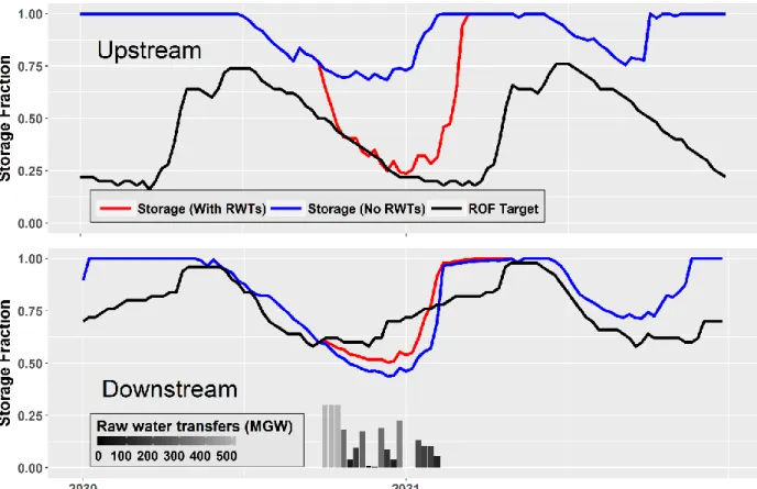
Figure 1: Example of raw water transfers at weekly intervals over a two-year period between an upstream donor (top) and downstream recipient (bottom). Raw water transfers (RWTs) are initiated if downstream storage levels fall below the downstream party risk-of-failure tolerance trigger (black, bottom) and upstream storage levels are above the upstream party risk-of-failure trigger level (black, top).
Should a raw water transfer (RWT) take place, the downstream party will initially request the full volume of water necessary to restore their reservoir storage downstream to risk-of-failure trigger storage levels (Figure 1; bottom, dotted line). This request, and all subsequent
operation – reservoirs operated by the U.S. Army Corps of Engineers (USACE), for instance, may impound or release water to maintain water quality and reduce flood risk as well as for water supply, meaning water allocated for supply is only a fraction of reservoir inflows. So, if 500 million gallons (MG) of water are required to raise supply storage levels and reduce downstream risk-of-failure to trigger levels, but only 50% of RWTs are allocated for water supply (an allocation ratio of 0.5), then a 1,000 MG RWT is requested. Reservoir releases to maintain downstream flow targets – natural flows required under environmental regulations – are not counted within RWT calculations. If downstream reservoir levels are below the failure level (20% of capacity) in any week, all RWT volume during that week is allocated for downstream water supply (allocation ratio of 1.0).
once non-supply needs are satisfied in a RWT week, any further RWT water allocated for those sectors is diverted for water supply, or alternatively the total request is curtailed after factoring in the new temporary allocation ratio of RWT allocation. Because RWTs will temporarily increase streamflows between upstream and downstream reservoirs, a cap on the volume of water
available for release in a single week will also be specified. This cap is sensitive to the historic streamflow magnitudes and shifts so as to avoid the potential of flooding.
The remaining RWT request amount is then finalized, with the agreed-upon amount released from upstream supply and added to downstream supply, according to the set
downstream water supply allocation ratio. The RWT is paid for by the downstream party the amount equal to the number of gallons of water transferred multiplied by a fixed price per volume of water transferred. The upstream party is then compensated by this amount.
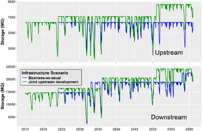
JUD capacity allocation would be available for transfer downstream at any time. The result of this storage arrangement can provide alternate futures of water management for upstream and downstream parties (Figure 2).
Figure 2: Example of potential upstream and downstream differences in storage capacity
between scenarios with (green) and without (blue) joint upstream infrastructure development. In this joint development case, upstream and downstream parties cooperate to expand capacity by 2025 and again in 2052.
2.2 Study area and modeling framework
utilities – Raleigh, Durham, Cary, and Orange Water and Sewer Authority (OWASA) – facing water scarcity challenges in the near future, the Triangle is a suitable test bed as a reflection of the similarly at-risk and densely-populated Eastern U.S. (GAO, 2014). Raleigh, the largest and fastest-growing city in the Triangle, is directly downstream from the City of Durham within the Neuse River Basin; these cities will act as the upstream (Durham) and downstream (Raleigh) parties to raw water transfers originating from Durham’s Lake Michie water supply reservoir and moving downstream into Falls Lake, Raleigh’s primary water supply source. Falls Lake,
Figure 3: The Research Triangle region of North Carolina in the eastern United States. Existing treated water infrastructure and potential raw water transfer activities highlighted.
Both utilities currently use risk-of-failure to trigger short-term interventions – water use restrictions and treated water transfers from Jordan Lake in the Cape Fear River Basin – as well as long-term infrastructure projects. While Durham has the ability to return wastewater effluent to the Cape Fear River Basin in substantial quantities, Raleigh does not, meaning any treated water transferred to Raleigh from Jordan Lake is considered an inter-basin transfer.
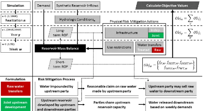
Triangle framework operates at several temporal scales (Figure 4). A model run, or simulation, is subject to a fixed set of decision parameters; these include risk-of-failure triggers for water transfers, use restrictions, and infrastructure as well as the raw water transfer allocation ratio and maximum weekly cap. Each simulation computes 1,000 realizations of the Triangle system from 2015 to 2060, evaluating utility decision-making and performance under unique, synthetic hydrologic “states-of-the-world” (Herman et al., 2013). Doing so allows a determination of the robustness of formulations and decision parameters across a wide range of potential future hydrologic and water demand scenarios (Kasprzyk et al., 2012; Reed et al., 2013). The synthetic hydrologic projections are based on inflows to Triangle reservoirs, generated through a re-creation of statistical moments and seasonal patterns in the historic record at several streamflow gages within the region using an auto-correlated bootstrapping technique (Kirsch et al., 2013). Projections of future demand growth are based on utility-provided estimations of annual growth and historical records of seasonal trends. Weekly demand is varied using a joint probability density function with observed inflow to develop a distribution of possible deviations from the weekly mean for each utility, which is then randomly sampled and the value is applied to adjust week-to-week demand.
risk-of-failure rise to specified decision trigger levels. For additional detail on risk-of-risk-of-failure and streamflow and demand projections in the Triangle system, see Zeff et al. 2016.
Figure 4: Triangle water supply model. Processes detailed based on temporal resolution (left of vertical solid line, separated by horizontal dashed lines) and formulation (colors, bottom rows). The business-as-usual simulation formulation involves all processes in grey, the raw water transfer formulation adds mitigation actions in red, and the joint upstream development formulation includes both red and green risk mitigation actions.
approved by all involved regulatory bodies, has ended; permitting period lengths were
determined based on conversations with and reports by regional water utilities. Once a project is implemented, it takes 3-5 years to be completed at which point the storage or production of that project is added to the participating utilities’ water supply budget. The cost of each option is spread over 25 years as debt service payment on bonds with 4% interest rates, parameters which are set based on consultation with Triangle water utility officials. For jointly-developed projects between two utilities, the fraction of project cost covered by a utility is exactly proportionate to that utility’s stake in production or capacity of the infrastructure option.
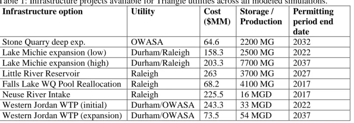
Table 1: Infrastructure projects available for Triangle utilities across all modeled simulations.
Infrastructure option Utility Cost
($MM) Storage / Production Permitting period end date
Stone Quarry deep exp. OWASA 64.6 2200 MG 2032
Lake Michie expansion (low) Durham/Raleigh 158.3 2500 MG 2022 Lake Michie expansion (high) Durham/Raleigh 203.3 7700 MG 2037
Little River Reservoir Raleigh 263 3700 MG 2027
Falls Lake WQ Pool Reallocation Raleigh 68.2 4100 MG 2017
Neuse River Intake Raleigh 225.5 16 MGD 2017
Western Jordan WTP (initial) Durham/OWASA 243.3 33 MGD 2022 Western Jordan WTP (expansion) Durham/OWASA 73.5 54 MGD 2037
reservoir with Raleigh paying for and owning a share of the increased capacity. Each formulation will be tested over a number of model simulations, with every simulation having different values selected for decision parameters such as risk-of-failure trigger levels, the maximum raw water transfer allowed in a given week, and the downstream allocation ratio.
Consistent through all formulations will be the independent infrastructure projects available to each utility, based on regional reports on future water supply planning (Table 1; TJCOG, 2014) and past modeling of optimal infrastructure pathways for regional sustainability (Zeff et al., 2016). To emphasize the potential benefits of raw water transfers and joint upstream development within the Triangle system, the following infrastructure options are made available: OWASA may choose to expand the smallest of its three reservoirs (Stone Quarry), while Raleigh may implement up to three primary supply enhancement options (reallocation of the Falls Lake water quality pool for water supply storage, construction of an intake to draw water from the Neuse River, or creation of a reservoir along Little River) and Durham, not including potential joint upstream development in model formulation (2), can opt along with OWASA to access an allocation of Jordan Lake by financing a water treatment plant to divert and treat the water and distribution mains to transport it to the utility.
2.3 Impacts of raw water transfers
hedge against low storage levels upstream by temporarily reducing water demands, typically by restricting outdoor water usage, in order to maintain supply reliability. Conversely, if a
downstream party were to request raw water transfers, but was denied, it is likely to seek water from another source, perhaps outside its watershed (an inter-basin transfer), potentially raising legal and environmental opposition. And, if short-term mitigation options are limited,
ineffective, or unavailable, a utility may be forced to expand its infrastructure in order to ensure reliable supply to cover infrequent and short-lived drought events, increasing their debt burden and likely raising water rates for customers. It is essential, therefore, to monitor the impact of raw water transfers across a number of objectives for both the upstream and downstream utilities. Assessment of raw water transfers based on their ability to satisfy objectives of
1. reliability 𝑓𝐹
2. use restriction frequency 𝑓𝑅𝐸𝑆𝑇 3. peak infrastructure debt burden 𝑓𝐷𝐸𝐵𝑇 4. risk of financial losses 𝑓𝐿𝑂𝑆𝑆
5. inter-basin treated water transfer use 𝑓𝑇𝑊𝑇
will evaluate the merit of raw water transfers in physical, economic, and financial terms, as well as illuminate any trade-offs between objectives that may arise as a result.
reliability, will represent the region as the objective value 𝑓𝐹 for the entire simulation (3). Each objective is mathematically described below:
The reliability (failure rate) objective is determined for a simulation by maximizing the worst-case failure rate among realizations r and utilities U and across years y. 𝐹 is either 0 or 1 depending on the existence of weekly storage failure in year y as described in (2). As with each objective, reliability is calculated separately for each utility U and the worst-performing utility represents the objective value (3).
min 𝑓𝐹 = max𝑈[∑
max𝑦(𝐹𝑟,𝑈,𝑦) 𝑛 𝑛
𝑟=1
] (3)
Restriction use frequency is quantified as the average percentage of weeks under
restriction by the worst-performing utility in the worst year of each realization of a simulation. 𝑅 represents the percentage of weeks under restriction in year y for utility U in realization r (4). Water utilities are often under political and public pressure to avoid implementing restrictions, making reduced restriction frequency a priority.
min 𝑓𝑅𝐸𝑆𝑇 = max𝑈[∑max𝑦(𝑅𝑟,𝑈,𝑦) 𝑛 𝑛
𝑟=1
] (4)
𝐴𝑉𝑅. The peak debt objective represents the average worst year debt ratio over all realizations (5). Bond payments are subject to the length of bond financing and interest rates for a utility.
min 𝑓𝐷𝐸𝐵𝑇 = 𝑚𝑎𝑥𝑈
[ ∑
𝑚𝑎𝑥𝑦(𝐴𝑉𝑅𝐵𝑃𝑟,𝑈,𝑦 𝑟,𝑈,𝑦) 𝑛
𝑛
𝑟=1
]
(5)
The potential for short-term supply shortfall mitigation strategies to destabilize utility revenues – use restrictions, for example, temporarily reduce revenues – means that minimizing transfers and use restrictions is crucial (Hughes and Leurig, 2013). To measure potential financial risk due to revenue losses, the financial losses objective represents the costs of short-term mitigation 𝑆𝑇𝑀, as a fraction of annual volumetric revenue, not expected to be exceeded in 99% of years through a simulation (6). Though the financial loss objective calculates value-at-risk for each utility that results from implementing short-term mitigation actions, this study did not include any measures the utility might take to mitigate those financial losses (i.e. reserve funds, financial insurance).
min 𝑓𝐿𝑂𝑆𝑆 = 𝑚𝑎𝑥𝑈[(𝑆𝑇𝑀𝑟: 𝑃{𝑆𝑇𝑀𝑟 > 𝑆𝑇𝑀} = 0.01)𝑈] (6)
𝑆𝑇𝑀𝑟,𝑈 = max𝑦
(max (𝑅𝐸𝑆𝑇𝐶𝑟,𝑈,𝑦+ 𝑇𝑊𝑇𝐶𝑟,𝑈,𝑦+ 𝑅𝑊𝑇𝐶𝑟,𝑈,𝑦, 0) 𝐴𝑉𝑅𝑟,𝑈,𝑦
(7)
For any utility purchasing on treated, inter-basin water transfers, there are both financial and political incentives to reduce reliance on this exchange. To quantify use of treated water transfers by the downstream party of raw water transfers, the treated water transfers objective represents average treated transfers 𝑇𝑊𝑇 to the downstream utility in the worst year of each realization over a simulation (8).
min 𝑓𝑇𝑊𝑇 = max𝑈[∑max𝑦(𝑇𝑊𝑇𝑟,𝑈,𝑦) 𝑛
𝑛
𝑟=1
CHAPTER 3: RESULTS
3.1 Objective performance across formulations
One-hundred and thirty-five model simulations across 3 formulations were run, each with a different set of parameter combinations (Table 2) and available infrastructure options. Figure 5A details the objective performance of each simulation to allow for visual comparison; each simulation is represented by a line across all five objectives with the ideal solution being a flat line across the bottom of the figure. Objective results for all 405 simulations are averaged by formulation in Table 3, Set A.
While patterns between formulations are difficult to visually discern in the entire objective set, trends in results are more apparent when downstream development by Raleigh is limited to one infrastructure option (Neuse River Intake) in Figure 5B (Table 3, Set B). These simulations are henceforth referred to as “low-development” simulations. In low-development simulations on average, formulations with temporary raw water transfers added, but no joint upstream development (Figure 5B, red), reduce the regional failure rate objective from 4.5% to 3.4%, cut use restriction frequency from 43% to 38% of weeks and marginally decrease
downstream treated transfer use in the worst simulation year relative to the business-as-usual (BAU) formulation (Figure 5B, blue) while maintaining the peak debt burden objective.
years with many transfer requests. Objective improvements persisted for the joint upstream development formulation (Figure 5B, green); relative to BAU, JUD formulations with limited downstream development lowered failure rate from 4.5% to 1.7%, worst-year restriction
frequency from 43% to 18% of weeks, and worst year downstream treated transfer use by 85%. Furthermore, peak debt burden decreased from 252% of AVR in the worst year to 238% AVR, while financial risk only rose by 0.2% of AVR. It should be noted that neither OWASA nor Cary utilities were drivers of the objective results, meaning objective values for either Durham or Raleigh – the two parties involved in raw water transfers – were reported as the worst regional result in all cases.
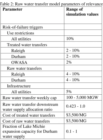
Table 2: Raw water transfer model parameters of relevance
Parameter Range of
simulation values
Risk-of-failure triggers Use restrictions
All utilities 10%
Treated water transfers
Raleigh 2 - 10%
Durham 2 - 10%
OWASA 2%
Raw water transfers
Raleigh 4 - 10%
Durham 4 - 10%
Infrastructure
All utilities 5%
Raw water transfer weekly cap 100 - 5,000 MGW Raw water transfer downstream
water supply allocation ratio 0.423 - 1.0 Cost of treated water transfers $3,500/MG Cost of raw water transfers $3,500/MG Fraction of Lake Michie
expansion capacity for Durham water supply
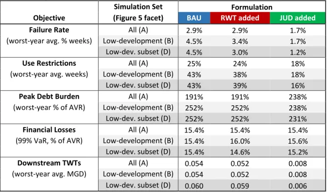
Table 3: Comparison table for subsets of simulation objective results, averaged by formulation
Simulation Set Formulation
Objective (Figure 5 facet) BAU RWT added JUD added
Failure Rate All (A) 2.9% 2.9% 1.7%
(worst-year avg. % weeks) Low-development (B) 4.5% 3.4% 1.7%
Low-dev. subset (D) 4.5% 3.0% 1.2%
Use Restrictions All (A) 25% 24% 18%
(worst-year avg. weeks) Low-development (B) 43% 38% 18%
Low-dev. subset (D) 43% 39% 16%
Peak Debt Burden All (A) 191% 191% 238%
(worst-year % of AVR) Low-development (B) 252% 252% 238%
Low-dev. subset (D) 252% 252% 231%
Financial Losses All (A) 15.4% 15.4% 15.4%
(99% VaR, % of AVR) Low-development (B) 15.4% 16.0% 15.6%
Low-dev. subset (D) 15.4% 14.6% 15.2%
Downstream TWTs All (A) 0.054 0.052 0.008
(worst-year avg. MGD) Low-development (B) 0.054 0.052 0.008
Low-dev. subset (D) 0.060 0.059 0.006
One indicator of particular importance to water utilities is their ability to maintain high levels of reliability. When considering only simulations from this study that experience failure in less than 1.5% of weeks in the worst average year, joint upstream development formulation simulations greatly outnumbered, 95 to 4, simulations of the business-as-usual formulation (Figure 5C). Though all joint upstream development formulations had greater average worst-year peak debt compared to business-as-usual formulations, due to cooperative Lake Michie
Figure 5: Parallel axis plots of objective performance across business-as-usual (blue), temporary raw water transfer (red) and joint upstream development (green) in sets of: (A) all computed simulations (B) low-development simulations only (C) all simulations with under 1.5% of worst realization years in failure (D) select low-development simulations. Objectives of failure rate (far left column), use restriction frequency (first column from left), peak annual infrastructure debt (middle column), financial risk (first from right), and treated water transfers to Raleigh (far right column) are determined from the worst-case year results over a model simulation. Ideal objective performance would be marked by a straight line across the bottom of the plot.
For further analysis, Figure 5B was distilled to three simulations representative of the distribution of low-development results in Figure 5D (Table 3, Set D). Each simulation in (D) has the same decision parameters and infrastructure options, the only difference being the
formulation. Improvement across all objectives, by both the RWT and JUD formulations relative to BAU, demarcate the possible benefits of raw water transfer use. Though not all simulations tested had such clear trends between formulations, this subset of results displays the potential of raw water transfer schemes when implemented effectively; both RWT and JUD formulations objectively dominate the business-as-usual formulation. With regard to utility supply reliability, raw water transfer and joint infrastructure development formulations improve upon the business-as-usual formulation (Figure 5D, left column) by reducing failure rate from 4.5% to 3.0% and 1.2% respectively. Under business-as-usual conditions this high rate of failure would be
low-development simulation subset, both peak debt and financial risk objectives were either maintained or improved by RWT and JUD formulations relative to BAU; regional worst-year peak debt is reduced by 21% of AVR by the JUD formulation relative to BAU, while both RWT and JUD formulations reduce financial risk from the 15.4% AVR levels of the BAU formulation.
3.2 Tradeoffs between upstream and downstream parties
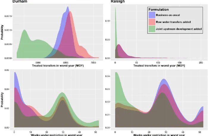
When the objective results of Figure 5D are dis-aggregated to show realization results within each simulation, it is evident that notable tradeoffs exist across objective performance between upstream (Durham) and downstream (Raleigh) parties to raw water transfers (Figure 6). Comparison of model formulations using distributions of restriction frequency and treated water transfers for each utility in a simulation, representing the worst year in each of the 1,000
realizations, demonstrated shifts across objectives. The upstream party to raw water transfers saw increases in restriction frequency and treated water transfer volume relative to the business-as-usual, no raw water transfer formulation, while the downstream party saw a decrease in use restriction frequency (Figure 6, differences between red and blue distributions). This is directly attributable to the exchange of raw water from Durham to Raleigh; raw water transfers reduce storage capacity in upstream reservoirs, more use restrictions are put in place and more treated water transfers are requested in response to this increased risk-of-failure. The downstream effects are opposite, where lower risk-of-failure levels as a result of increased reservoir inflows from raw water transfers mean fewer use restrictions are enacted. Though raw water transfer and joint upstream development formulations clearly shift risk from the downstream to the upstream party, regional objective performance improves (Figure 5D) relative to business-as-usual. This
upstream reservoir capacity, Durham (the upstream party) does not suffer objectively while providing downstream objective improvement due to more efficient use of available resources.
Figure 6: Comparison of model formulations through distributions of treated transfer volume (top) and use restriction frequency (bottom) in the worst year of each of 1,000 realizations within a single simulation for the upstream (Durham, left) and downstream (Raleigh, right) parties to raw water transfers. Raw water transfer formulation results (red) show increased treated water transfers to and use restrictions by Durham but fewer use restrictions for Raleigh relative to business-as-usual (blue). Formulations also including joint upstream Lake Michie development (green) demonstrate increases in Durham and decreases in Raleigh use restriction frequency relative to business-as-usual and temporary raw water transfer formulations. Joint upstream development resulted in decreased treated water transfer use for both utilities relative to other formulations. Distributions of treated water transfers to Raleigh under business-as-usual and raw water transfer formulations were nearly identical, hence the appearance of a single, discolored distribution.
between utilities. Changes in Figure 6 between joint development (green) and alternative formulations show that upstream use restriction frequency in the worst year was greatest with joint upstream development relative to either business-as-usual or temporary raw water transfer formulations, while the opposite was true for downstream restriction frequency. While this is logical for downstream Raleigh – more storage capacity means lower risk-of-failure – Durham sees increasing restriction use even with added reservoir capacity. This has two causes:
differences in Durham’s necessity in the joint development formulation to expand Lake Michie should Raleigh come under risk-of-failure as well (in the business-as-usual formulation, Durham does not cooperate with Raleigh), and Durham’s capacity stake in Lake Michie expansion. These results show Lake Michie, able to expand to either a low or high level, being expanded to a small extent before 2025 when joint development is allowed. This means that Durham’s preferred independent expansion option, accessing an allocation of Jordan Lake, is pushed into the future relative to the business-as-usual scenario. This change in development is further strained
depending on the size of Durham’s stake in the capacity of an expanded Lake Michie. For these results, Durham purchases only 30% of Lake Michie expansion capacity. The combined push to expand Lake Michie by Raleigh, driven by Raleigh’s large future demands, with Durham waiting longer to tap a larger, independent supply means Durham must enact more use restrictions to deal with worst-case hydrologic conditions.
3.3 Implications for inter-basin transfer
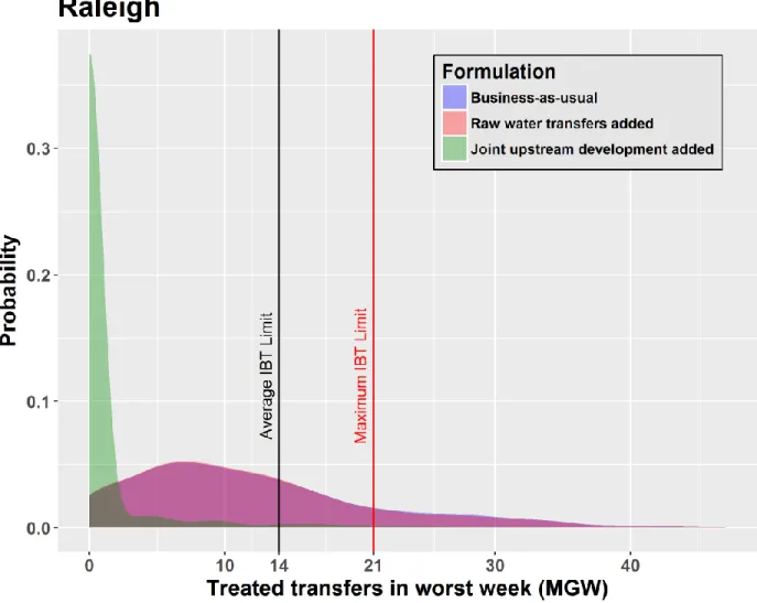
transfers from Jordan Lake with additional firm capacity in Lake Michie, and similarly Raleigh avoids the need to purchase emergency treated water transfers from Jordan Lake (diverted and treated by Cary before being piped through existing interconnections) in worst cases. Joint upstream development showed the ability to reduce treated water transfers to Raleigh by at least 85% on average relative to BAU, and by 90% in the low-development simulation subset (Figure 5D).
the world (Figure 7, green), with only 1% (13) of 1,000 realizations violating the 21 MG worst-week inter-basin transfer threshold.
Figure 7: Comparison of model formulations treated inter-basin transfer in the worst week of each of 1,000 realizations within a single simulation for the downstream (Raleigh) party to raw water transfers. NC municipalities are required to receive governmental approval for inter-basin transfers of over 3 MGD (red line) or 2 MGD (black line) on average. Joint upstream
CHAPTER 4: DISCUSSION
The potential for raw water transfer schemes to improve the flexibility of eastern U.S. water management flexibility is not solely limited to the NC Research Triangle. Though this type of raw water exchange, to the authors’ knowledge, has not been extensively used outside of the Western U.S., we find evidence that it can be applied within existing Eastern institutions, largely because many state laws regarding water use are old and purposefully vague. So long as
upstream impoundments do not reduce downstream river flows so as to deprive riparian users of their right to the resource – something that would not occur as a result of increased flows from raw water transfers – the financial and reliability benefits afforded by raw water transfers, creating an additional supply augmentation strategy while reducing regional infrastructure use, appear to demonstrate considerable potential.
noted that this analysis was not an optimization of decision variables surrounding raw water transfers, and the results portrayed demonstrate the potential of raw water transfers and joint upstream development to improve regional objectives, but do not fully characterize the Triangle system. Future efforts will couple large-scale optimization of raw water transfer decision-making with sensitivity analysis of relevant parameters to confidently scope the potential for raw water transfers and joint development to positively influence water management.
CHAPTER 5: CONCLUSIONS
The ability to combine raw water transfer schemes with existing water management policy in the eastern U.S. may be valuable for regions with rising populations seeking to meet water demands. Reduced reliance upon traditional, structural solutions to limit water supply shortfalls through more flexible use of existing capacity and regional cooperation will be
REFERENCES
Abrams, R. H. (1982). Interbasin in a Riparian Jurisdiction. Wm. & Mary L. Rev., 24, 591. Adkins, J., Miller, S., Rouse, R., and Westbrook, V. (2016, May 6). Personal meeting with
Triangle utility members.
Baerenklau, K. A., Schwabe, K. A., & Dinar, A. (2014). The residential water demand effect of increasing block rate water budgets. Land Economics, 90(4), 683-699.
Caldwell, C., & Characklis, G. W. (2014). Impact of contract structure and risk aversion on interutility water transfer agreements. Journal of Water Resources Planning and Management, 140(1), 100-111.
Characklis, G. W., Kirsch, B. R., Ramsey, J., Dillard, K. E., & Kelley, C. T. (2006). Developing portfolios of water supply transfers. Water Resources Research, 42(5).
Gargan, H. (2017, February 7). Judge rules in favor of Fayetteville, against Cary and Apex in Jordan Lake water lawsuit. Raleigh News & Observer.
Government Accountability Office (2014). Freshwater: Supply Concerns Continue, and Uncertainties Complicate Planning. United States Government, GAO-14-430. Getches, D. H. (1997). Water law in a nutshell. West Pub. Co. 3.
Gleick, P. H. (2003). Global freshwater resources: soft-path solutions for the 21st century.
Science, 302(5650), 1524-1528.
Gleick, P. H., & Palaniappan, M. (2010). Peak water limits to freshwater withdrawal and use.
Proceedings of the National Academy of Sciences, 107(25), 11155-11162.
Herman, J. D., Reed, P. M., Zeff, H. B., & Characklis, G. W. (2015). How should robustness be defined for water systems planning under change?. Journal of Water Resources Planning and Management, 141(10), 04015012.
Hughes, J. A., and S. Leurig (2013), Assessing Water System Revenue Risk: Considerations for Market Analysts, Ceres, Boston, Mass.
Israel, M., & Lund, J. R. (1995). Recent California water transfers: Implications for water management. Nat. Resources J., 35, 1.
Triangle J Council of Governments (2014). Triangle Regional Water Supply Plan: Volume II: Regional Water Supply Alternatives Analysis. TJCOG.
Kasprzyk, J. R., Reed, P. M., Kirsch, B. R., & Characklis, G. W. (2009). Managing population and drought risks using many‐objective water portfolio planning under uncertainty.
Water Resources Research, 45(12).
Kirsch, B. R., Characklis, G. W., & Zeff, H. B. (2012). Evaluating the impact of alternative hydro-climate scenarios on transfer agreements: Practical improvement for generating synthetic streamflows. Journal of Water Resources Planning and Management, 139(4), 396-406.
Klein, C. A. (2008). Water Transfers: The Case Against Transbasin Diversions in the Eastern States. 25 UCLA J. Envtl. L. & Pol'y 249.
Leurig, S. (2010). The Ripple Effect: Water Risk in the Municipal Bond Market. Ceres, Boston, Mass.
Lund, J. R. (2015), Integrating social and physical sciences in water management, Water Resour. Res., 51, 5905–5918, doi:10.1002/2015WR017125.
McLawhorn, D. F. and Maddux, J. (2009). Water Ownership by N.C. Local Governments.
University of North Carolina at Chapel Hill School of Government.
Moncur, J. E. (1987). Urban water pricing and drought management. Water Resources Research,
23(3), 393-398. N.C. Gen. Stat. § 143-215.44
National Research Council (1992). Water Transfers in the West: Efficiency, Equity, and the Environment. National Academy Press, Washington D.C.
National Research Council (2004). Confronting the Nation’s Water Problems: The Role of Research. National Academy Press, Washington D.C.
National Research Council (2012). Challenges and Opportunities in the Hydrologic Sciences.
National Academy Press, Washington, D.C.
Olmstead, S. M., & Stavins, R. N. (2009). Comparing price and nonprice approaches to urban water conservation. Water Resources Research, 45(4).
Palmer, R. N., & Characklis, G. W. (2009). Reducing the costs of meeting regional water demand through risk-based transfer agreements. Journal of environmental management,
Postel, S. L., Daily, G. C., & Ehrlich, P. R. (1996). Human appropriation of renewable fresh water. Science, 271(5250), 785.
Reed, P. M., Hadka, D., Herman, J. D., Kasprzyk, J. R., & Kollat, J. B. (2013). Evolutionary multiobjective optimization in water resources: The past, present, and future. Advances in water resources, 51, 438-456.
Renwick, M. E., & Green, R. D. (2000). Do residential water demand side management policies measure up? An analysis of eight California water agencies. Journal of Environmental Economics and Management, 40(1), 37-55.
Vaux, H. J., & Howitt, R. E. (1984). Managing water scarcity: an evaluation of interregional transfers. Water resources research, 20(7), 785-792.
Va. Code Ann. § 62.1-115
Wilchfort, O., & Lund, J. R. (1997). Shortage management modeling for urban water supply systems. Journal of water resources planning and management, 123(4), 250-258.
Zeff, H. B., Kasprzyk, J. R., Herman, J. D., Reed, P. M., & Characklis, G. W. (2014). Navigating financial and supply reliability tradeoffs in regional drought management portfolios.
Water Resources Research, 50(6), 4906-4923.
Zeff, H. B., Herman, J. D., Reed, P. M., & Characklis, G. W. (2016). Cooperative drought adaptation: Integrating infrastructure development, conservation, and water transfers into adaptive policy pathways. Water Resources Research, 52(9), 7327-7346.