TECHNICAL UNIVERSITY OF CLUJ-NAPOCA
ACTA TECHNICA NAPOCENSIS
Series: Applied Mathematics, Mechanics, and Engineering Vol. 61, Issue III, September, 2018
INCORPORATING BILL OF MATERIALS IN BOTTOM-UP DEMAND
FORECASTING
Mehmet GULSEN
Abstract: In a manufacturing environment, the final product includes sub-assemblies and elementary parts that are put together hierarchically. By using hierarchy information in the bill of materials (BOM), demand forecasts for sub-assemblies and elementary parts can be generated from the final product. If an elementary part is used in multiple products, there will be several forecasts for the same part. The volatility of the aggregate forecast is expected to be higher as each product has its own independent demand pattern. An alternative approach is to reverse the process: first aggregate the historical data, then generate the forecasts. Hierarchical information from the bill of materials can be used for aggregation.
Key words: Hierarchical forecasting, bill of materials, forecast accuracy, bottom-up forecasting).
1. INTRODUCTION
Accuracy in demand forecasting is an important issue that directly impacts the bottom line of a corporation. Most of the operational activities in a company are scheduled according to anticipated future demand. Production planning in manufacturing facilities and procurement of raw materials are all dependent on expected future sales. Any deviation or miscalculation in demand forecast will appear as operational inefficiencies with a potential financial loss. Overestimation of demand will lead to excess inventory, and underutilization of manufacturing means as materialized demand would be smaller than what company had originally anticipated. Additionally, it will lead to the procurement of excessive input material which will end up as extra stock in the company’s warehouse. On the other hand, underestimation of demand will also have a damaging effect on the company’s operation, with the even worse financial loss. Underestimation of demand will lead to raw material shortages, and overextension and overuse of available manufacturing means. The company will not be able to fill orders which will
result in lost sales and, more importantly, the loss of customer goodwill.
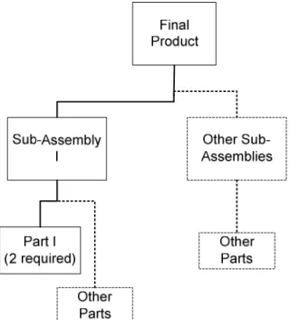
in its simplest definition, is an extensive list of raw materials and components that are required to build a product. Each item in the list has an identification number and notes the quantity required. It also includes hierarchical information which shows how parts come together to form the final product. Figure 1 graphically shows BOM for a product with sub-assemblies and individual parts. Two units of Part I are used in building this product.
Fig. 1. Graphical representation of BOM.
In forecasting demand for low-level items, forecasts for final products are often propagated to the lower levels. For example, if the expected demand for the final product is 10 units, the forecast for the part I would simply be: 2 times 10, 20 units. Overall demand for part 1 can be calculated by summing the demand for the part I at each product. This is a simple method, but it does not necessarily give an accurate forecast.
2. LITERATURE
Data aggregation is frequently used in forecasting to reduce the variability of the input data. Having less variability in the input data leads to more stable (i.e., less variance) forecasts. In a stable data set, it is easier to identify underlying trends and seasonality of the series. This is the primary motivation for data aggregation in forecasting [13] [4][12].
Aggregation can be performed on different dimensions of the data. Location, product
characteristics and time are the most commonly used dimensions to aggregate data. For location, the geographical position of customers or suppliers is often used as a basis for aggregation. Location-wise, grouping is also called spatial aggregation. Product aggregation requires combining different items into a single basket based on one or more common characteristics of the items. Data aggregation over time is performed by rolling data from a low-frequency period to a longer one. For example, hourly data may be rolled up to a daily level to create longer frequency data. This is particularly true if the original data set is sparsely populated with many periods containing zero observations [8].
Product aggregation is the most commonly used aggregation form used in forecasting [14]. Most of the time products have inherent hierarchical characteristics that could be exploited for aggregation. For example, a polo shirt comes in different colors, sizes, and cuts which could be used as parameters for potential product aggregation. Hierarchical product aggregation is used in two distinct approaches: bottom-up and top-down forecasting.
In a bottom-up approach, forecasts are generated at the lowest level (i.e., SKU levels), then they are rolled up to a higher level. In a top-down approach, forecasts are generated at a higher level, then they are dis-aggregated to lower levels. Of course, there is an issue of how to prorate the aggregate forecast to the lower levels (i.e., SKU level). There are some works in this are addressing the prorating issue [10].
Temporal aggregation refers to aggregating data from a lower frequency time series to a higher frequency (hourly data is rolled up to a daily level). Especially within the context of intermittent demand, accumulating demand in longer time buckets reduces the number of periods with zero demand, and the aggregated series will have periods populated with non-zero demand [14].
Temporal aggregation is commonly used in a time series to smooth-out the seasonality effect. If a monthly series is aggregated to an annual series, the variance in the data set due to seasonality is eliminated, and any variance in the aggregated data is due to trend and cycle components [7]. In the literature, temporal aggregation is used successfully for demand forecasting purposes [11],[2],[1].
3. EMPIRICAL EVALUATION
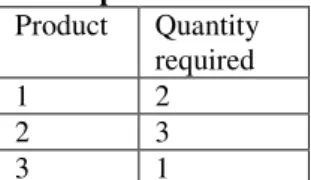
In our forecasting approach, we use BOM information to collect historical demand data for low-level input materials. For illustrative purposes, let’s assume that a company produces three products. A common input material is used in each product. The number of input materials required for each product is given in Table 1.
Table 1: Number of input material required for each product.
Product Quantity required
1 2
2 3
3 1
One way of forecasting demand for the input material is to use a top-down approach. First, generate forecasts for final products. Then, by using information from BOM, propagate forecasts to lower level items. This approach is especially preferred if forecasts for final products are already generated for some other purpose (e.g., sale estimates for marketing). When forecasts for final products are already available, it is tempting to use available estimates for lower level items. However, this approach does not necessarily give the best results.
To show why a top-down approach does not always work, we compare it to our proposed method. In the first approach, we will use the conventional method where final product forecasts plus BOM information are used to generate forecasts for low-level input items. In the second approach, we will aggregate historical demand for low-level input items. The forecast model will use the aggregate historical data to generate the forecasts. The sum of forecasts from the first approach is compared to the forecast generated from the aggregate data.
3.1 Data Sets
The data set includes three products with six years of monthly demand data. The first five years of data is used for model development. The last 12 observations are kept for validation. Two closed-form functions are used to create simulated demand data (equation 1 & 2). The first one is a damped exponential function with two parameters, A and b, representing the level and the damping rate. The demand data for Product 1 in our test runs are generated by using the damped exponential function. Here, the demand rises faster initially, but the rate of increase damps as time progresses. The coefficient b defines the dampening rate of the demand. As t gets larger, the demand converges to a level represented by A. The second function is a linear equation with an intercept and a slope(b). The demand data for products 2 and 3 are generated by using the linear equation. A stable demand with a slight negative slope is used for the second product while the third product has a growing demand with a positive slope.
Damped Exponential Function: (1 bt) e A Y = − −
(1)
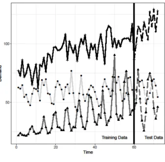
Fig. 2. Demand profiles for three products.
The final demand profiles in Figure 2 are generated by applying seasonality and random noise on function outputs. For seasonality, we use a vector of 12 elements representing the relative magnitude of demand in each month. The numbers in the vector give the ratio of demand in a particular month to the average monthly number for the whole year. After the adjustment for seasonality, random noise is added to the data. Multiplicative noise factors are generated by using the normal distribution (i.e., 1+N(0,σ) ).
3.2. Forecasting Technique
The monthly demand is a time-series data with a trend and a seasonality. To forecast demand for future months, we use an exponential smoothing approach with trend and seasonality. This approach is called Holt-Winter’s method for the namesake of its inventors [9]. It is an averaging method where the forecast is based on the average of past observation. Unlike simple averaging where each observation has equal weight, the weight values in exponential smoothing follow an exponentially declining pattern from most the recent observation to the distant ones.
The Holt-Winter method is an extension of the simple exponential smoothing forecast model (equation 3), the forecast for the next period is a
function of the most recent forecast (Ft) and
forecast error (Yt −Ft)of the last period. The model takes the last forecast and updates it for the next period by using forecast error.
Simple Exponential Smoothing:
) (
1 t t t
t F Y F
F+ = +
α
− (3)The Holt-Winter method adds a trend and a seasonality component to the simple exponential smoothing method. m s t t t t s t t t t t t t t t t s t t S m b L F S L Y S b L L b b L S Y + − − − − − − + = − + = − + − = + − + = ) ( : Forecast ) 1 ( Seasonal ) 1 ( ) ( : Trend ) )( 1 ( L : Level 1 1 1 t
γ
γ
β
β
α
α
4. COMPUTATIONAL RESULTS
We tested our approach on ten different randomly generated data sets. We compare the proposed approach to an alternate top-down approach, which is a conventional way of low-level forecasting items. In the conventional forecasting, forecasts for the final products are generated in the first stage. Forecasts for final products and BOM information are used to calculate for the lower-level items.
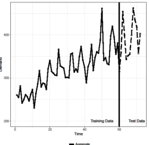
The results for each approach are shown in Figure 2 and Figure 3 respectively. The historical data is shown in solid lines whereas the dotted lines represent forecasts. In Figure 2, each final product’s historical demand and corresponding forecasts are given separately. The forecast for the low-level item is calculated in two steps: (1) Low-level item forecast is generated for each product by using BOM information, (2) Sum of low-level forecasts over all products gives the total need for the low-level item. Figure 3 shows the aggregate historical data (solid line) and forecasting based on this aggregate data (dotted line). The sum from the first approach is directly compared to forecasts given in Figure 3.
Fig. 3. Aggregate history for the low-level item and the forecast.
Table 2: Absolute error deviation for two approaches
Test Run
Conventional Approach
Proposed Approach
Difference
1 596.7 324.2 45.7%
2 489.2 433.4 11.4%
3 635.5 596.8 6.1%
4 414.2 179.6 56.6%
5 497.5 392.1 21.2%
6 469.0 266.0 43.3%
7 503.0 313.8 37.6%
8 419.1 277.8 33.7%
9 465.0 289.8 37.7%
10 479.0 279.2 41.7%
5. CONCLUSION 
In this study, BOM information, which is readily available in most companies, is used to improve demand forecasting accuracy. The BOM a is a hierarchical list that defines components and raw materials used in a product. In forecasting demand for lower level components and raw materials, the top-level forecast for the final product is propagated to the lower levels with the help of BOM information. This a simple and intuitive method but that does not give accurate forecasts as it is shown in this study.
8. REFERENCES
[1] Babai, A., & Nikolopoulos, K., Impact of temporal aggregation on stock control performance of intermittent demand
estimators: Empirical analysis. Omega, 40(6), 713–721, (2012).
[2] Boylan, J., E., & Babai, M., Z., On the performance of overlapping and non-overlapping temporal demand aggregation approaches. 181(SI) 136-144, (2016).
[3] Chen, H., & Boylan, J.E., Use of individual and group seasonal indices in sub-aggregate demand forecasting. Journal Operations Research Society. 58, 1660–1671, (2007). [4] Chopra, S., & Meindl, P., Supply chain
management: strategy, planning, and operations. Fourth edition. Pearson. (2010). [5] Huber, J., & Gossmann, A., &
Stuckenschmidt, H. Cluster-based hierarchical demand forecasting for perishable goods. Expert Systems with Applications, 76, 140–151, (2017).
[6] Kourentzes, N., & Petropoulos, F., Forecasting with multivariate temporal aggregation: The case of promotional modeling. International Journal of Production Economics, 181, 145–153, (2016).
[7] Kourentzes, N., & Rostami-Tabar, B., & Barrow, D. K., Demand forecasting by temporal aggregation: Using optimal or multiple aggregation levels? Journal of Business Research 78, 1–9, (2017).
[8] Nikolopoulos, K., and Syntetos, A.A., and Boylan, J.E., and Petropoulos F., and Assimakopoulos, V., An aggregate– disaggregate intermittent demand approach (ADIDA) to forecasting: an empirical proposition and analysis. Journal of the Operational Research Society 62, 544 –554, (2011).
[9] Makridakis, S. and Wheelwright, S.C. and Hyndman, R.J. Forecasting, methods and applications, Third Edition, John Wiley and Sons. (1998)
[10] Pennings, C.L.P., & van Dalen, J., (2017). Integrated hierarchical forecasting. European Journal of Operational Research. 263 412– 418, (2017).
[12] Russel, R. S., & Taylor, B. W., Operations and supply chain management. Eighth edition. Wiley. (2014).
[13] Simchi-Levi, D., & Kaminsky, P., & Simchi-Levi, E., Designing and managing the supply chain: concepts, strategies and case studies. McGraw Hill, International Edition, (2009).
[14] Syntetos. A.A., & Babai, Z., & Boylan, J. E., & Kolassa, S., & Nikolopoulos, K.,
Supply chain forecasting: Theory, practice, their gap and the future. European Journal of Operational Research, (252), 1-26,
[15] Zotteri, G., & Kalchschmidt, M., & Caniato, F., The impact of aggregation level on forecasting performance. International Journal Production Economics 93–94 (2005) 479–491, (2005).
ÎNCORPOREAZĂ LISTĂ DE MATERIALE ÎN PROGNOZAREA CERERII
DE JOS ÎN SUS
Rezumat: Într-un mediu de fabricație, produsul final include subansamble și elemente elementare
care sunt puse împreună în mod ierarhic. Prin utilizarea informațiilor de ierarhie în factura de material
(BOM), previziunile cererii pentru subansambluri și piese elementare pot fi generate din produsul
final. Dacă o componentă elementară este utilizată în mai multe produse, vor exista mai multe
previziuni pentru aceeași parte. Volatilitatea prognozei agregate este de așteptat să fie mai ridicată,
deoarece fiecare produs are propriul model de cerere independent. O abordare alternativă este de a
inversa procesul: mai întâi agregați datele istorice, apoi generați prognozele. Informațiile ierarhice
din contul de materiale pot fi utilizate pentru agregare.