CAS: Property-Liability Insurance Loss Reserve Ranges Based on Economic Value

Reserve Ranges Based on Economic

Value

by Stephen P. D’Arcy, Alfred Au, and Liang Zhang

ABSTRACT

A number of methods to measure the variability of

property-liability loss reserves have been developed to meet the

re-quirements of regulators, rating agencies, and management.

These methods focus on nominal, undiscounted reserves, in

line with statutory reserve requirements. Recently, though,

there has been a trend to consider the fair value, or

eco-nomic value, of loss reserves. Insurance regulators

world-wide are starting to consider the economic value of loss

reserves, which reflects how much needs to be set aside

today to settle these claims, instead of focusing on

nomi-nal values. If insurers switch to economic values for loss

reserves, then reserve variability would need to be

calcu-lated on this basis as well. This approach will add

consid-erable complexity to reserve variability calculations. This

paper combines loss reserve variability and economic

val-uation. Loss reserve ranges are calculated on a nominal

and economic basis for a simplified insurer to illustrate the

key variables that impact loss reserve variability. Nominal

interest rate and inflation volatility, interest rate-inflation

correlation, and the relationship between claim cost and

general inflation are key factors that affect economic loss

reserve variability. Actuaries will need to focus on

mea-suring these values accurately if insurers adopt economic

valuation of loss reserves.

1. Introduction

Traditional loss reserving approaches in the property-casualty field produced a single point estimate value. Although no one truly expects losses to develop at exactly the stated value, the focus was on a single value for reserves that did not reflect the uncertainty inherent in the process. As the use of stochastic models in the insurance industry grew, for dynamic financial analysis (DFA), for asset liability management (ALM) and other advanced financial techniques, loss reserve variability became an important is-sue. McClenahan (2003) describes the history of interest in reserve variability and loss reserve ranges. Hettinger (2006) surveys the different ap-proaches used to establish reserve ranges. The CAS Working Party on Quantifying Variability in Reserve Estimates (2005) provides a detailed description of the issue of reserve variability, in-cluding an extensive bibliography and set of is-sues that still need to be addressed. The conclu-sions of this Working Party are that despite ex-tensive research on this area to date there is no clear consensus within the actuarial profession as to the appropriate approach for measuring this uncertainty, and that much additional work needs to be done in this area. All of the approaches described in this report, and suggestions for fu-ture research, focus on measuring uncertainty in statutory loss reserves. Given recent attention to fair value insurance accounting, future research should also focus on more accurate economic re-serve ranges.

The use of nominal values for loss reserves is sometimes justified as providing a safety load, or risk margin, over the true (economic) value of the reserves. However, risk margins determined in this way would fluctuate with interest rates and vary by loss payout patterns. A more ap-propriate approach, which is beyond the scope of this research, would be to establish risk mar-gins based on the risks inherent in the reserve estimation process, such as determining the risk

margin based on the difference between the ex-pected economic value and a level such as the 75th percentile value.

The Financial Accounting Standards Board (FASB) and the International Accounting Stan-dards Board (IASB) have proposed an alterna-tive approach to valuing insurance liabilities, in-cluding loss reserves. This approach, termed fair value, proposes that loss reserves in financial re-ports be set at a level that reflects the value that would exist if these liabilities were sold to an-other party in an arms length transaction. The relative infrequency with which these exchanges actually take place, and the confidentiality sur-rounding most trades that do occur, make this approach to valuation more of a theoretical ex-ercise than a practical one, at least in the cur-rent environment. However, fair value would re-flect the time value of money, so the trend would be to set loss reserves at their economic rather than nominal values if these proposals are imple-mented. The issues involved, and financial im-plications, in fair value accounting are covered extensively in the Casualty Actuarial Society re-port,Fair Value of P&C Liabilities: Practical Im-plications (2004). However, despite the comphensive nature of the papers included in this re-port, little attention is paid to the impact the use of fair value accounting would have on loss re-serve ranges. If rere-serves are to be calculated on a fair value basis, then reserve ranges should also be based on this approach as well.

cred-ibility. The report of the Task Force on Actuarial Credibility (2005) included the recommendation that actuarial valuations include ranges to indi-cate the level of uncertainty in the reserving pro-cess, and that additional work be done to clarify what the ranges indicate. Once again, the focus was on statutory loss reserve indications, rather than the economic value.

The critical problem with setting reserve ranges based on nominal values is the impact of inflation on loss development. Based on rela-tively recent history (the 1970s) and current eco-nomic conditions (increasing international de-mand for raw materials, vulnerable oil supplies, the U.S. Federal Reserve’s response to the sub-prime credit crisis), increasing inflation has to be accorded some probability of occurring in the future by any actuary calculating loss reserve ranges. As inflation will affect all lines of busi-ness simultaneously, the impact of sustained high inflation would be to cause significant adverse loss reserve development for property-liability insurers. Loss reserve ranges based on nominal values would therefore include the high values that would be caused by a significant rise in in-flation. However, inflation and interest rates are closely related, as first observed by Irving Fisher (1930) and confirmed by economists consistently since. The loss reserves impacted by high infla-tion would most likely be accompanied by high interest rates, so the economic value of those re-serves would not be that much higher than the economic value of the point estimate for reserves. Using economic values to determine reserve ranges could also lead to narrower ranges and provide a clearer estimate of the true financial impact of reserve uncertainty.

This project utilizes realistic stochastic models for interest rates, inflation, and loss development to determine loss reserve distributions and ranges on both a nominal and economic basis, draws a comparison between the two approaches, and explains why the appropriate measure of

uncer-tainty is based on the economic value. This work builds on prior work by Ahlgrim, D’Arcy, and Gorvett (2005) developing a financial scenario generator for the CAS and SOA as well as re-search on the interest sensitivity of loss reserves by D’Arcy and Gorvett (2000) and Ahlgrim, D’Arcy, and Gorvett (2004).

This study measures the uncertainty in loss reserving that is based on process risk, the in-herent variability of a known stochastic process. In this analysis, both the distribution of losses and the parameters of the distributions are given. Thus, unlike actual loss reserving applications, there is no model risk or parameter risk. Setting loss reserves in practice involves more degrees of uncertainty, and would therefore lead to greater variability in the underlying distributions of ulti-mate losses and larger reserve ranges. This study is meant to illustrate the difference between nom-inal and economic ranges, and starting with spec-ified loss distributions more clearly demonstrates this effect.

2. Review of loss reserving

methods

discus-sions on the strengths and weaknesses of vari-ous evaluation models include Zehnwirth (1994), Narayan and Warthen (1997), Barnett and Zehn-wirth (1998), Patel and Raws (1998), and Kirsch-ner, Kerley, and Isaacs (2002). These works typ-ically deal with nominal undiscounted value of loss reserves in line with statutory reserve re-quirements. Shapland (2003) explores the mean-ing of “reasonable” loss reserves, emphasizmean-ing the need for models to take into account the var-ious risks involved along with “reasonable” as-sumptions. His paper points out that reasonable-ness is subject to many aspects, such as culture, guidelines, availability of information, and the audience; as such the paper concludes that more specific input is needed on what should be con-sidered “reasonable” in the actuarial profession. Traditional methods use imbedded historical inflation to produce the nominal reserves. Out-standing losses will be exposed to the impact of inflation until they are finally paid. If the infla-tion rate during the experience period has been high, loss severity will be projected to be high generating large loss reserves. Similarly, after pe-riods of low inflation, loss severity will be pro-jected to increase more slowly, leading to lower loss reserves. Because inflation and interest rates are correlated, an insurer with an effective Asset Liability Management (ALM) strategy for deal-ing with interest rate risk can alleviate some of the impact of changing inflation.

There have been reserving techniques that at-tempt to isolate the inflationary component from the other effects, such as those proposed by But-sic (1981), Richards (1981), and Taylor (1977). Butsic investigated the effect of inflation upon incurred losses and loss reserves, as well as the inflation effect on investment income. For both increases and decreases in inflation, these com-ponents are found to vary proportionally. Ac-cording to Butsic, as competitive pricing is de-pendent on a combination of both claim costs and investment income, insurers are to a large

extent unaffected by unanticipated changes in in-flation. Richards provides a simplified technique to evaluate the impact of inflation on loss re-serves by factoring out inflation from historical loss data. Assumptions of future inflation can then be factored in to project possible values of future loss reserves. Under the Taylor sepa-ration method, loss development is divided into two components, inflation and superimposed in-flation. This method assumes the inflation com-ponent affects all loss payments made in a given year to the same degree, regardless of the orig-inal accident year. Essentially, unpaid losses are not considered to be fixed in value over time but rather are fully sensitive to inflation. An alterna-tive to this assumption is proposed by D’Arcy and Gorvett (2000), which allows loss reserves to gradually become “fixed” in value from the time of the loss to the time of settlement. In-flation would only affect the unpaid losses that have not yet become fixed in value. These two methods will be described in detail in the model section.

3. Asset liability management

respond differently, the firm will be exposed to interest rate risk. Prior to the 1970s, mismatches between assets and liabilities were not a signif-icant concern. Interest rates in the United States experienced only minor fluctuations, making any losses due to asset-liability mismatch insignifi-cant. However the late 1970s and early 1980s were a period of high and volatile interest rates, making ALM a necessity for any viable financial institution. If interest rates increase, fixed income bonds decrease in value and the economic value (the discounted value of future loss payments) of the loss reserves decreases. The opposite oc-curs for both the assets and liabilities when inter-est rates decrease. Ahlgrim, D’Arcy, and Gorvett (2004) provide a detailed analysis of the effective duration and convexity of liabilities for property-liability insurers under stochastic interest rates that shows how assets can be invested to reduce the impact of interest rate risk.

Insurers can employ an ALM program to re-duce the impact of inflation on loss reserves and maintain their surplus with changing interest rates. This requires insurers with short effective duration liabilities to hold short-term assets. Some insurers invest in longer duration assets that offer higher yields. During periods of sta-ble or declining interest rates, this approach will provide a higher return. However, when inter-est rates rise this strategy can be costly.1 The effect of duration mismatching on loss reserves given expectations of future inflation volatility is a complicated issue, and is outside the scope of this paper. As will be shown later, the higher the correlation between nominal interest rates and in-flation, such as in the 1970s, the more important and significant ALM’s impact will be.

1_{In late 2007 and early 2008, many banks suffered significant losses}

by following a similar mismatched strategy. They used off balance sheet structured investment vehicles (SIV) that invested in long-term bonds, often tied to subprime mortgages, but financed the investments with short-term debt. When the value of the assets fell and the credit markets froze up increasing short-term borrowing costs, the banks incurred significant losses which, in some cases, cost the CEOs their jobs (Hilsenrath 2008).

4. Economic value of loss

reserves

Recent developments by the Financial Ac-counting Standards Board (FASB) and the Inter-national Accounting Standards Committee (IASC) have advocated fair value accounting measures. The American Academy of Actuaries established the Fair Value Task Force to address this issue. The fair value of a financial asset or li-ability is its market value, or the market value of a similar asset or liability plus some adjustments. If a market does not exist, the asset or liability should be discounted to its present value at an appropriate capitalization rate depending on the risk components it encompasses. The Fair Value report by AAA (2002) provides details on the valuation principles. The promotion of fair value accounting, which considers both risk and the time value of money, indicates a new trend to-wards economic valuation.

The trend towards economic or market value based measurement of the balance sheet replac-ing existreplac-ing accountreplac-ing measures is also seen in the European Union, where solvency regulation is currently under reform. The European insur-ance and reinsurinsur-ance federation, CEA (2007), describes how the new Solvency II project takes an integrated risk approach which will better ac-count for the risks an insurer is exposed to than the current fixed standards under Solvency I. Sol-vency II introduces the use of a market-consistent valuation of assets and liabilities and market con-sistent reserve valuation, much like those pro-posed under fair value accounting in the United States.

observ-Figure 1. Annual observed inflation since 1930

able market-based rates. These rates are based on characteristics of the future obligations, or de-rived from a yield of a replicating portfolio of low-risk securities. The study mentions that ap-propriate allowance can be made for future claim escalation from inflation and superimposed in-flation (e.g. social or legal costs), but no clear methodology is provided as to how inflation should be taken into account.

Although there has been much discussion on the meaning of fair or economic value, both with-in and outside the United States, little attention has been given so far to the impact of economic value on loss reserve ranges. This paper ties to-gether the loss reserve ranges with the economic values to show the relationship between loss re-serve ranges on a nominal and economic basis and to illustrate some of the issues involved in calculating reserve ranges on economic values.

The economic value of an insurer’s liabilities is determined by discounting expected future cash flows emanating from the liabilities by their appropriate discount rate. Butsic (1988) and D’Arcy (1987) explore discounting reserves us-ing a risk-adjusted interest rate which reflects the risk inherent in the outstanding reserve.

Girard (2002) evaluates this using the company’s cost of capital. Actuarial Standard of Practice No. 20 (Actuarial Standards Board 1992) addresses issues actuaries should consider in determining discounted loss reserves. This standard suggests that possible discount factors could be the risk-free interest rate or the discount rate used in asset valuation.

5. Trends in inflation level and

volatility

Inflation as measured by the 12-month change in the Consumer Price Index (CPI) has varied widely, from ¡11% to +20% over the period 1922 through 2007 (Figure 1). Since the adop-tion of Keynesian economic policies in devel-oped countries following World War II, the gen-eral trend has been to avoid deflation at the cost of persistent inflation.2 Rapid increases in oil prices in the 1970s and the early 21st century

2_{There is some disagreement over how much of an impact}

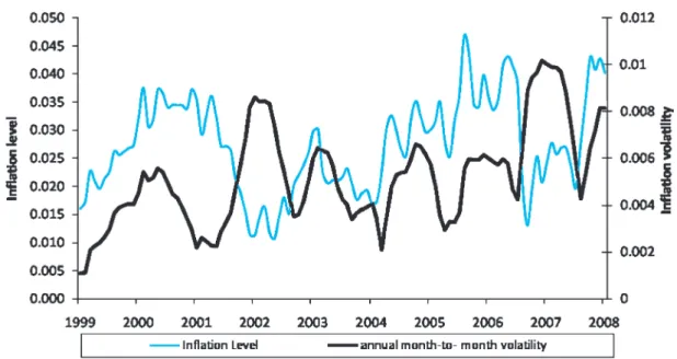
Figure 2. Annualized monthly observed inflation since 1999

have increased inflation rates. The steady depre-ciation of the dollar in recent years has also put additional inflationary pressures on the U.S. economy. Recently, concern over the financial consequences of the subprime mortgage crisis and credit crunch has led the U.S. Federal Re-serve to lower the discount rate to shield the economy from a housing slump and stabilize tur-bulence in the financial markets. Lowering inter-est rates is likely to lead to an increase in future inflation. Oil prices have risen sharply, the dollar has dropped to historical lows against the euro and gold prices have soared. Falling prices of long-term government debt after the recent rate drop suggests investors concern over inflation. Thus, the potential for inflation to increase must be incorporated into any financial forecast.

Figure 1 shows the inflation level and the in-flation volatility (based on a ten-year moving av-erage) since 1930. Inflation volatility, similar to interest rate volatility in interest rate models, is the standard deviation of the inflation rate over a one-year period. The ten-year moving average inflation volatility is calculated based on infla-tion rates over the last 120 months. The inflainfla-tion rate is determined by the CPI at the end of each

month compared to the CPI one year prior. Note the periods of deflation that occurred during the Depression and right after World War II, and the inflation spikes of the 1940s, 1950s, 1970s, and 1980s. Inflation volatility has also experienced several spikes, most recently in the 1980s. For the last decade, volatility has been at historic lows. Figure 2 shows the same data from the past 10 years, where there appears to be a rise in both inflation and inflation volatility. On this graph, inflation volatility is shown on a year-by-year basis (using only the last 12 months of data) to show the recent volatility more clearly. With the current upward trend in inflation volatility, it is necessary to consider the possibility infla-tion volatility returning to the levels of the 1950s or the 1980s. Inflation volatility determines how accurately we are able to predict future infla-tion trends; the greater the volatility, the lower the ability to forecast future inflation, and thus the greater uncertainty on its impact on loss re-serves.

6. The models

a two-factor Hull-White model for nominal terest rates, a OrnsteUhlenbeck model for in-flation, adjustment for correlation between the nominal interest rate and inflation, adjustment for claims cost inflation, and a fixed claims model for the impact of inflation on unpaid claims model. A sensitivity analysis worksheet is also built in to test the sensitivity of the parameters.

6.1. Loss generation model

The loss generation model generates aggregate claims based on the user’s input of the num-ber of claims, choice of distribution of the claim severity, and the mean and standard deviation of severity. The number of claims is assumed to be known. The severity of claims can follow a Nor-mal, Log-normal or Pareto distribution.

6.2. Loss decay model

These losses can be settled either at a fixed time or at a rate based on a decay model over a number of years. If the claims are to be settled on a decaying basis, the decay model calculates the proportion of losses to be settled each year given a decay factor. For simplicity, loss severity is as-sumed to be independent of time to settlement. The decay model is of the following form:

X_t+1= (1¡®)¤X_t (6.1) where X_i is the number of claims settled in year i, and ®is the decay factor or the proportion of claims settled each year.

6.3. Nominal interest rate model

A two-factor Hull-White model is used to gen-erate nominal interest rate paths. The Hull-White model uses a mean-reverting process with the short-term real interest rate reverting to a long-term real interest rate, which is itself stochastic and reverting to a long-term average level.

dr_t=·_r(l_t¡r_t)dt+¾_rdz_r

dl_t=·_l(¹_¡l_t)dt+¾_ldz_l (6.2)

where t is the time, r is the short-term rate, l is the long-term rate,·is the mean reversion speed, ¹ is the average mean reversion level, dt is the time step, ¾ is the volatility and dz is a Wiener process. This model allows for negative values, which is not theoretically possible for nominal interest rates. We impose a minimum short-term and long-term rate of 0% to adjust for this.

6.4. Inflation model

A one-factor Ornstein-Uhlenbeck model is used to generate inflation paths. The Ornstein-Uhlenbeck model uses a mean-reverting process with the current short-term inflation reverting to the long-term mean.

dr_t=·_r(¹_r¡r_t)dt+¾_rdz_r, (6.3) wheretis the time,ris the current inflation,· is the mean reversion speed,¹is the long-term in-flation mean,dtis the time step,¾is the volatility and dz is a Wiener process.

6.5. Correlated nominal and real

interest rates

The short-term nominal interest rate and in-flation rates are correlated through their random shock components. The randomdzcomponent is adjusted for a weighted average between a com-mon correlated random component and an indi-vidual random component.

dz_r,nominal=½dz_correlated+

q

1¡½2_dz nominal

(6.4)

dz_r,inflation=½dz_correlated+

q

1¡½2_dz inflation

where ½ is the correlation factor between the short-term interest rate and inflation rate, and dz are Wiener processes.

6.6. Masterson Claims Cost Index

over time by decomposing the costs into its var-ious components and inflating each part sepa-rately (Masterson 1981; Masterson 1987; Van Ark 1996; Pecora 2005). For this research, the Masterson Claim Cost Index is simplified to a linear projection of the inflation rate.

6.7. Fixed claim model

Cash flows from unpaid claims are sensitive to inflation rate changes. Under the Taylor separa-tion model (1977), any claim that has not been settled is subject to the full inflation in that year. If there is a car accident now and the claimant receives ongoing medical treatment for several years before the loss is settled, all medical costs are assumed to be impacted by inflation until the claim is paid. D’Arcy and Gorvett (2000) pro-pose a model that reflects a different relation-ship between unpaid losses and inflation. Their model separates unpaid claims into portions that are “fixed” in value from those which are not. These fixed claims, once determined, will not be subject to future inflation while the remaining unfixed claims continue to be exposed to infla-tion. For example, medical treatment given over a period of time becomes fixed in value when the service is provided. If medical prices rise af-ter some treatment has been provided, only fu-ture medical treatment will have this increased cost; medical treatment received before the price increase will have already been fixed. Any pain and suffering compensation is generally deter-mined at a later date. This portion of the claim will likely continue to be affected by inflation until this claim is settled. As a result of only exposing partial loss segments to inflation, in-flation’s impact on the loss is greatly reduced. A representative function that displays these at-tributes is:

f(t) =k+f(1¡k_¡m)(t=T)ng (6.5) where f(t) represents the proportion of the ulti-mate claims “fixed” at timet,kis the proportion

of the claim that is fixed immediately, m is the proportion of the claim that will be fixed only when the claim is settled, and T is the time at which the claim is fully settled.

The model (6.5) can be divided into three cases by the value of the exponent n: the linear case n= 1, when claim value is fixed uniformly up to its ultimate settlement; the convex casen >1, when the rate of fixing the value of a claim in-creases over time, and the concave case n <1, when the rate of fixing the value of a claim in-creases quickly initially but slows down as time approaches the ultimate settlement date. The larger the n, the more closely the fixed claim model will resemble the Taylor model.

7. Parameterization

Based on the ten-year loss development data of the auto insurance industry from A. M. Best’s Aggregate and Averages over the period 1980— 1996, approximately one-half of all remaining losses of the total loss value are settled each year up to the ultimate settlement year. Assuming loss severity to be independent of time of settlement, we use a decay factor ®= 0:5 for the number of claims settled each year. If loss severity is positively correlated with time of settlement, we would use a larger decay factor for the number of claims settled, but offset that by increasing the value of claims over time. Calculating the decay factor based on total loss value adjusts for the as-sumption that claims severity is independent of time to settlement.

Regressions were run against historical data to parameterize the Ornstein-Uhlenbeck inflation model and the two-factor Hull-White nominal in-terest rate model. These parameters are tabulated below:

Ornstein-Uhlenbeck

Inflation Model Two-Factor Hull-White Nominal InterestRate Model

· ¹ § ·_r ¹ ¾_r ·_l ¾_l

The Fisher formula is an equilibrium statement that, on average, nominal rates and inflation are linked. Sarte (1998) has found that in an envi-ronment with stochastic inflation, the Fisher for-mula is still a reasonable approximation to its more complete counterpart in a dynamic endow-ment environendow-ment. It is also worthy to note that inflation is a matter of government policy rather than just a fact of nature; and the model should be adjusted to match the current economic situ-ation.

The correlation between the three-month U.S. Treasury interest rates (the shortest securities is-sued) and percentage changes in the CPI index was determined for several periods as shown be-low. The relationship between inflation and in-terest rates hypothesized by Fisher applies to ex-pected inflation and current interest rates. There is no reliable measure of expected inflation, so the actual inflation rate for a recent period is used here instead. The CPI is an estimate of a mar-ket basmar-ket of prices at a particular time; monthly changes include significant noise, as under or over-stated values in one month are adjusted the following month. This leads to the lowest val-ues for the correlations. Inflation rates calculated based on three and six month CPI changes are more highly correlated with interest rates. The problem introduced by increasing the time pe-riod for determining the current inflation rate is that these rates may be less indicative of expected inflation. To run the model, we selected the one month inflation value over the more recent time period, or 45%. Other values for this correlation are shown in the sensitivity tests.

Correlation between 3-month treasury bill rate and inflation

Years 1934–2007 1934–1970 1971–2007 One-Month Inflation Rates 0.241 0.007 0.459 Three-Month Inflation Rates 0.317 0.006 0.556 Six-Month Inflation Rates 0.364 0.011 0.615 Twelve-Month Inflation Rates 0.414 ¡0:007 0.684

The Masterson Claims Cost Index for auto in-surance bodily injury from 1936 to 2004 was

regressed against the historical inflation rate us-ing a fixed intercept of 0. The slope of the re-gression increases over time indicating that claim costs have been increasing more than CPI infla-tion benchmarks. A slope of 1.6 was selected for this model; other values are illustrated in the sen-sitivity section.

For the fixed claim model, we are using the linear case, with the parameter for k (portion of claim fixed at inception of claim) of 0.15 as sug-gested in D’Arcy and Gorvett (2000), but the parameter for m (portion of the claim fixed at settlement) at 0.5. The sensitivity of these values is examined in a later section.

8. Running the model

This model is available on the author’s Web site and will also be made available through the CAS Web site so any interested reader can run the model to reproduce the results here or test alternative parameters. The loss reserve model, which is designed in Microsoft Excel, begins with an input worksheet for the user to enter the parameters for each model used and the number of iterations to be made in the simulation. For each iteration, the model generates a loss distri-bution, a nominal interest rate path, and an infla-tion path, which are used to produce the nominal and economic loss ranges. An output worksheet collects the values from each iteration run and calculates the mean, standard deviation, and re-serve ranges for both the nominal and economic value cases. The summary sheet collects these key statistics, the parameters used, and the num-ber of iterations in the simulation in side-by-side columns for comparison.

The generated losses are compounded at the inflation rate up to their time of settlement. This is the nominal, undiscounted value of losses that insurers are statutorily required to have as a re-serve. The interest rate model generates cumu-lative interest rate paths corresponding to each time period up to settlement. The nominal val-ues are then discounted back by this cumulative interest rate factor to obtain the economic value of losses.

For a simplified example, assume a single claim of $1,000 (based on the price level in effect when the loss occurred) is settled at the end of five years, and the annual nominal interest rate is 5%. Also assume that the inflation is equal to one half of the nominal rate throughout the five years, i.e., (1 + 5%)0:5¡1 = 0:0247. The nomi-nal value of the loss reserve would be $1,000¤

(1 + 2:47%)5= $1129:73. This nominal value is discounted back by the interest rate over the five years to get the economic value $1129:73¤

(1 + 5%)¡5= $885:17. In economic terms, the amount that should be reserved for handling this loss in today’s dollars is $885.17. Now consider what would happen if interest rates changed by 200 basis points up or down. If the nominal rate is 7%, inflation will be (1 + 7%)0:5

¡1 = 3:44%, and the nominal value and econ-omic value will be $1,184.30 and $844.39, re-spectively. If the nominal rate is 3%, inflation will be (1 + 3%)0:5¡1 = 1:49%, and the nominal value and economic value will be $1,076.70 and $928.77, respectively. Thus, the nominal value range will be $1, 129:73¡$1, 076:70 = $53:03, and the economic value range will be $928:77¡

$885:17 = $43:60. The economic value range is only 82% of the nominal value range. This is a simplified example illustrating three possible val-ues of one claim, assuming inflation is propor-tional to the nominal rate. Under circumstances like this, the reserve range based on economic values will be smaller than reserve ranges based on nominal values.

Now consider a book of 1,000 such claims and allow inflation to vary independently of nominal rates. The average nominal and economic val-ues of these 1,000 claims are determined based on the interest rate and inflation paths generated for that simulation. This claims generation pro-cess is repeated for 10,000 simulations, with each simulation generating a different interest rate and inflation path for the 1,000 claims of that itera-tion, and a distribution of nominal and economic loss reserves are generated. The mean, standard deviation, minimum, maximum, as well as the 5, 25, 75, and 95 percentile for both the nomi-nal and economic loss ranges are determined and compared. A confidence interval ratio is com-puted by dividing the economic range confidence interval by the nominal range confidence inter-val for both a 50 percent (ranging from the 25th percentile to the 75th percentile) and 90 percent (ranging from the 5th percentile to the 95th per-centile) confidence interval. These ratios will be used as an indicator of the difference in volatility between the economic loss ranges and nominal loss ranges.

9. Results

To examine the effects of how the confidence interval is affected by changes in the assump-tions, 10,000 simulations were run for each of the following cases. As the 50 percent and 90 percent confidence interval ratios turn out to be fairly close, only the 90 percent confidence inter-val ratios are shown here. The complete results are available from the authors. A monthly time step was chosen to provide a close approxima-tion to continuous interest rate models, as infla-tion data are only available monthly.

9.1. Taylor Model versus Fixed Claim

Model

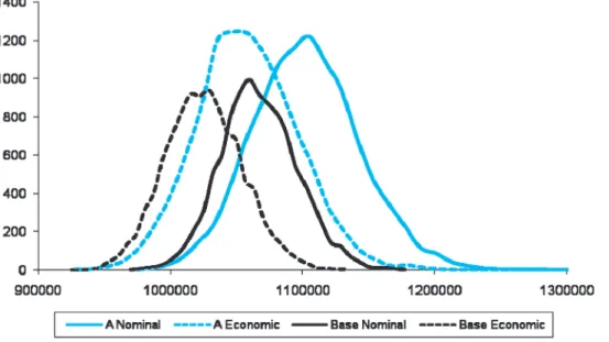
be-Figure 3. Taylor (blue) vs. fixed claim (base case, black)

Table 1. Summary values for Taylor model (A) and fixed claum model (B)

Standard Percentiles 90% Confidence Confidence

Case Mean Deviation 5th 95th Interval Interval Ratio A—nominal 1097016.132 40241.05642 1033427.88 1165584.07 132156.19 94.15% A—economic 1052020.311 37895.67459 991242.95 1115669.17 124426.22

B—nominal 1063890.967 28761.53405 1018485.77 1112663.88 94178.11 101.78% B—economic 1021643.248 29192.93832 974956.77 1070811.09 95854.32

tween the nominal interest rate and inflation, 3) claims inflation rate of 1.6 times the general inflation rate, 4) the Taylor separation model. This is Case A. Figure 3 shows the distribu-tions for both the nominal and economic values; as would be expected, the economic values are lower than the nominal values, but the economic reserve range turns out to be approximately 94% of the nominal loss reserve range. Discounting does not reduce the ranges much. The second ex-ample, Case B, incorporate the fixed loss model suggested by D’Arcy and Gorvett (2000). In this case there is a significant decrease in the standard deviation of the nominal and economic reserves because losses are only partially exposed to in-flation throughout its time to settlement. (Fixed claims are no longer affected by future inflation.) In this case the confidence interval ratio (the eco-nomic range divided by the nominal range) is

102%. Discounting reserves reduces the level of the reserves, but not the range. We will treat Case B as the base case and examine additional changes in relationship to this case. The mean values, standard deviations, 5th and 95th per-centiles and the 90% confidence intervals are for both nominal and economic values for Case A and Case B are shown on Table 1.

9.2. High claims cost inflation

infla-Figure 4. High claim inflation (blue) vs. base case (black)

Table 2. Summary values for high claim cost inflation

Standard Percentiles 90% Confidence Confidence

Case Mean Deviation 5th 95th Interval Interval Ratio C—nominal 1078069.12 33220.69 1025879.25 1134626.99 108747.74 96.89% C—economic 1034635.49 32372.86 983266.87 1088635.84 105368.97

tion. Recently, the relationship between claims cost and inflation as increased significantly; be-tween 2001 and 2004, auto bodily injury costs between increased 1.9 times the general infla-tion rate. For Case C, the claim cost inflainfla-tion factor will be 1.9 and the standard deviation of the nominal range will be increased 1.9 times the original inflation volatility. As the nominal range is the claims cost inflated value of the real loss, higher claims cost inflation will increase the nominal range and decrease the confidence inter-val ratio. The distributions for both the Base Case and Case C are shown on Figure 4, and the key metrics of Case C are shown on Table 2. For Case C the confidence interval ratio of the economic range to the nominal range drops to 97%.

9.3. High correlation between inflation

with nominal rates

Inflation and nominal interest rates moved in tandem during the 1970s, with correlation

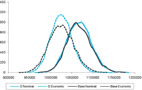
reach-ing 65% to 70%. Based on a 12-month infla-tion rate, the correlainfla-tion with interest rates over the period 1970—2007 was 68%. High correla-tion between inflacorrela-tion and nominal interest rates reduces the range of economic loss reserves. For Case D the correlation factor was 70%. Figure 5 shows how this increase in correlation has little impact on the nominal values of loss reserves, but does reduce the distribution of economic values. In this case, the confidence interval ratio drops to 88% (Table 3).

Figure 5. High correlation (blue) vs. base case (black)

Table 3. Summary values for high correlation between inflation and nominal interest rate

Standard Percentiles 90% Confidence Confidence

Case Mean Deviation 5th 95th Interval Interval Ratio D—nominal 1064157.75 28783.10 1018181.31 1112651.8 94470.49 88.40% D—economic 1021531.44 25496.24 980743.24 1064253.59 83510.35

Table 4. Summary values for high and volatile inflation

Standard Percentiles 90% Confidence Confidence

Case Mean Deviation 5th 95th Interval Interval Ratio E—nominal 1173532.64 97382.53 1036359.22 1351072.81 314713.59 87.50% E—economic 1121600.19 85091.77 1000580.60 1275965.70 275385.10

compared with the base case. Table 4 provides the key metrics for Case E; the confidence inter-vals are much wider and the confidence interval ratio is 88%.

9.5. Summary of results

Based on the many simulations run for this re-search, the economic mean is smaller than the nominal mean. Under most circumstances, the economic value reserve ranges are slightly smaller than the nominal value ranges. This is not always the case under the fixed claim model. The economic value range will be smaller than the nominal value ranges if claims cost inflation is very high relative to the CPI inflation, if

cor-relation is high between the nominal interest rate and inflation, or if inflation becomes highly volatile.

9.6. Sensitivity analysis

Figure 6. Volatile inflation (blue) vs. base case (black)

Table 5. Sensitivity analysis

Model Parameter From To Increment Results (ratios) 90% CI Range Type

Inflation Mean 2% 12% 2% No effect 98–101% N/A Inflation Speed 0.1 0.3 0.05 Increase 96–105% Linear Inflation Vol 1% 8% 1% Decrease 115–87% Concave Nominal LT Mean 2% 10% 2% No effect 99–103% N/A Nominal LT Speed 0.02 0.10 0.02 No effect 100–102% N/A Nominal LT Vol 0.6% 1.2% 0.2% No effect 100–101% N/A Nominal ST Speed 0.02 0.10 0.02 No effect 100–103% N/A Nominal ST Vol 1% 5% 1% Increase 96–141% Linear Fixed Claim K 0.1 0.4 0.1 Increase 99–105% Linear Fixed Claim M 0.3 0.8 0.1 Decrease 106–98% Linear Fixed Claim N 0.5 2 0.5 No effect 99–102% N/A

Loss SD 200 1000 200 No effect 98–101% Linear Decay Factor 0.2 0.8 0.1 Increase 92–102% Convex Correlation Correlation 0% 100% 20% Decrease 109–58% Convex Claim Cost Slope 0.4 2.0 0.4 Decrease 127–94% Linear

on the confidence interval range; in all cases, the economic value range was approximately 100% of the nominal value range. The next line indi-cates that changing the speed of mean reversion for the inflation rate over the range 0.1 to 0.3 increased the confidence interval range, in a lin-ear manner, from 96% to 105%. Based on these results, the factors that have the most effect on the relationship between the confidence interval

10. Conclusion

Property-liability insurance companies have traditionally valued their loss reserves on a nomi-nal basis due to statutory requirements. These re-quirements do not reflect the economic value of the future payments and distort insurance com-pany financial statements. Nominal loss reserves overstate the impact of inflation on reserves, though only slightly under the current economic environment, as they ignore the relationship be-tween inflation and nominal interest rates. The economic impact on loss reserves of a change in inflation is commonly offset by a similar shift in the nominal interest rate and by the high claims cost inflation. Loss reserve ranges based on nom-inal values accentuate this problem. Recent pro-posals advocate the use of fair value account-ing for loss reserves, which would replace nomi-nal values with economic values. In this study a loss reserve model was developed to quan-tify the uncertainty introduced by stochastic in-terest rates and inflation rates and to compare reserve ranges based on nominal and economic values. The results demonstrate a variety of sce-narios under which the reserve ranges based on economic values can be either smaller or larger than the nominal value ranges. However, use of economic values for loss reserves would better serve the insurance industry and its regulators. The key reason for encouraging the use of eco-nomic value ranges is that they properly reflect the true measure of the uncertainty involved in loss reserving. An additional benefit is that the ranges are smaller in many circumstances, and the current economic environment seems to be moving toward those situations. Claim cost in-flation and the level and volatility of inin-flation appear to have an upward trend. Economic value reserves would provide more credible values of the cost and uncertainty of future loss payments, and in the cases mentioned before, would have a smaller confidence interval range.

Acknowledgment

The authors wish to thank the Actuarial Foun-dation and the Casualty Actuarial Society for fi-nancial support for this research.

References

Actuarial Standards Board, Actuarial Standard of Practice No. 20, “Discounting of Property and Casualty Loss and Loss Adjustment Expense Reserves,” April 1992, http:// www.actuarialstandardsboard.org/pdf/asops/asop020 037.pdf.

Ahlgrim, Kevin, Stephen P. D’Arcy, and Richard W. Gorvett, “The Effective Duration and Convexity of Liabilities for Property-Liability Insurers Under Stochastic Interest Rates,”Geneva Papers on Risk and Insurance Theory29:1, 2004, pp. 75—108.

Ahlgrim, Kevin, Stephen P. D’Arcy, and Richard W. Gorvett, “Modeling Financial Scenarios: A Framework for the Ac-tuarial Profession,”Proceedings of the Casualty Actuarial Society92, 2005, pp. 60—98.

American Academy of Actuaries, “Fair Valuation of Insur-ance Liabilities: Principles and Methods,” 2002, http:// www.actuary.org/pdf/finreport/fairval sept02.pdf. Australian Prudential Regulation Authority, GPS 310,

“Au-dit and Actuarial Reporting and Valuation,” February 2006, http://www.apra.gov.au/General/upload/GPS-310-Audit-and-Actuarial-Valuation.pdf.

Barnett, Glen, and Ben Zehnwirth, “Best Estimates for Re-serves,” Casualty Actuarial SocietyForum, Fall 1998, pp. 1—54.

Berquist, James R., and Richard E. Sherman, “Loss Re-serve Adequacy. Testing: A Comprehensive, Systematic Approach,”Proceedings of the Casualty Actuarial Society

64, 1977, pp. 123—184.

Best’s Aggregates and Averages, Property-Casualty, A. M. Best, selected years.

Butsic, Robert P., “The Effect of Inflation on Losses and Premiums for Property-Liability Insurers,” Casualty Ac-tuarial Society Discussion Paper Program, 1981, pp. 58— 102.

Butsic, Robert P., “Determining the Proper Interest Rate for Loss Reserve Discounting: An Economic Approach,” Ca-sualty Actuarial SocietyDiscussion Paper Program, Fall 1988, pp. 147—186.

Casualty Actuarial Society, “Fair Value of P&C Liabili-ties: Practical Implications,” 2004, http://www.casact.org/ pubs/fairvalue/FairValueBook.pdf.

Casualty Actuarial Society, “Task Force on Actuarial Credi-bility,” 2005, http://www.casact.org/about/reports/tfacrpt. pdf.

CEA Information Papers, “Solvency II: Understanding the process,” 2007, http://www.cea.assur.org/cea/download/ publ/article257.pdf.

D’Arcy, Stephen P., “Revisions in Loss Reserving Tech-niques Necessary to Discount Property-Liability Loss Re-serves”Proceedings of the Casualty Actuarial Society74, 1987, pp. 75—100.

D’Arcy, Stephen and Richard W. Gorvett, “Measuring the Interest Rate Sensitivity of Loss Reserves,”Proceedings of the Casualty Actuarial Society87, 2000, pp. 365—400, http://www.casact.org/pubs/proceed/proceed00/00365. pdf.

Fisher, Irving,The Theory of Interest, New York: Macmillan, 1930, Ch. 19.

Girard, Luke N., “An Approach to Fair Valuation of Insur-ance Liabilities Using the Firm’s Cost of Capital,”North American Actuarial Journal6:2, 2002, pp. 18—46.

Hettinger, Thomas, “What Reserve Ranges Makes You Comfortable,” Midwestern Actuarial Forum Fall Meet-ing, 2006, http://www.casact.org/affiliates/maf/0906/ hettinger.pdf.

Hilsenrath, Jon, “When Nerves Get Short, Credit Gets Tight,”

Wall Street Journal, February 19, 2008, p. C 1.

Institute of Actuaries of Australia, Professional Standard 300, “Valuations of General Insurance Claims,” August 2007, http://www.actuaries.asn.au/NR/rdonlyres/0A2FF 56A-1489-404F-BBF3-CB7D916B269E/2908/PS300 ApprovedbyCouncil28August2008.pdf.

Kirschner, Gerald S., Colin Kerley, and Belinda Isaacs, “Two Approaches to Calculating Correlated Reserve In-dications Across Multiple Lines of Business,” Casualty Actuarial SocietyForum, Fall 2002, pp. 211—246.

Mack, Thomas, “Distribution-free Calculation of the Stan-dard Error of Chain Ladder Reserve Estimates,”ASTIN Bulletin23, 1993, pp. 213—225.

Masterson, Norton E., “Property-Casualty Insurance Infla-tion Indexes: Communicating with the Public,” Casualty Actuarial Society Discussion Paper Program, 1981, pp. 344—370.

Masterson, Norton E., “Economic Factors in Property/Casu-alty Insurance Claims Costs,”Best’s Review, June 1987, pp. 50—52.

McClenahan, Charles L., “Estimation and Application of Ranges of Reasonable Estimates,” Casualty Actuarial So-cietyForum, Fall, 2003, pp. 213—230.

Miller, Mary Frances, “Are You Part of the Solution,”

Actuarial Review31:2, February 2004, http://www.casact. org/pubs/actrev/feb04/pres.htm.

Murphy, Daniel M., “Unbiased Loss Development Factors,”

Proceedings of the Casualty Actuarial Society 81, 1994, pp. 154—222.

Narayan, Prakash, and Thomas V. Warthen, “A Compara-tive Study of the Performance of Loss Reserving Meth-ods Through Simulation,” Casualty Actuarial Society

Forum, Summer 1997, pp. 175—196.

Patel, Chandu C., and Alfred Raws, III, “Statistical Mod-eling Techniques for Reserve Ranges: A Simulation Ap-proach,” Casualty Actuarial Society Forum, Fall 1998, pp. 229—255.

Pecora, Jeremy P., “Setting the Pace,” Best’s Review, Jan-uary 2005, pp. 87—88.

Richards, William F., “Evaluating the Impact of Inflation on Loss Reserves,” Casualty Actuarial Society Discussion Paper Program, Fall 1981, pp. 384—400.

Sarte, Pierre-Daniel G., “Fisher’s Equation and the Infla-tion Risk Premium in a Simple Endowment Economy,”

Economic Quarterly84, Fall 1998, pp. 53—72.

Shapland, Mark R., “Loss Reserve Estimates: A Statistical Approach for Determining ‘Reasonableness’,” Casualty Actuarial SocietyForum, Fall 2003, pp. 321—360. Standard & Poor’s, “Insurance Actuaries: A Crisis of

Cred-ibility,” 2003.

Taylor, Greg C., “Separation of Inflation and Other Effects from the Distribution of Non-Life Insurance Claim De-lays,”ASTIN Bulletin9, 1977, pp. 219—230.

Van Ark, William R., “Gap in Claims Cost Trends Contin-ues to Narrow,”Best’s Review, March 1996, pp. 22—23. Venter, Gary G., “Refining Reserve Runoff Ranges,”ASTIN

Colloquium, Orlando, FL, 2007.

Wiser, Ronald F., Jo Ellen Cockley, and Andrea Gardner, “Loss Reserving”Foundations of Casualty Actuarial Sci-ence, Casualty Actuarial Society, 2001, Ch. 5, pp. 197— 285.

Zehnwirth, Ben, “Probabilistic Development Factor Models with Applications to Loss Reserve Variability, Prediction Intervals, and Risk Based Capital,” Casualty Actuarial SocietyForum, Spring 1994, pp. 447—606.

Appendix—Sensitivity Analysis

Instead, we ran the model multiple times for se-lected numbers of simulations and then calcu-lated the variability of the 90% confidence inter-val ratio, the key variable used in this study. (This value is the ratio of the 90% confidence interval based on the economic value of loss reserves to the 90% confidence interval based on the nomi-nal value of loss reserves.) For each number of simulations, the model was run eight times and the coefficient of variation of the confidence in-terval ratios was calculated (Table 1-A). The op-timal number of simulations was the point where the coefficient of variation did not continue to decline when additional simulations were run. The starting point was 1,000 simulations, which generated a coefficient of variation of 2.83%. The number of simulations was increased, first to 2,500, then 5,000 and 7,500. The coefficient of variation gradually declined to 1.12%. Running 10,000 simulations did not reduce the variability further, so this combination (10,000 simulations of 1,000 claims) was used to run the individual cases (A through E) described in the paper.

Due to limitation in computational power, a smaller number of simulations were used to run the sensitivity analyses. As this required multi-ple runs for each variable over a range of feasi-ble values, we used 5,000 simulations and 1,000 claims for this aspect of the project. Although the coefficient of variation of the 90% confidence in-terval ratios was slightly higher for this combina-tion, at 1.61%, this was still sufficient to show the general effect of changing each parameter over the relevant range.

Table 2-A shows the level of the variable changed and the corresponding 90% confidence interval ratio for each sensitivity test. The long-term mean inflation rate was varied from 2% to 12%, but in each case the confidence interval ratio remained approximately 100%. This value exhibited no trend over this range. Varying the

Table 1-A. Sensitivity analysis for the number of simulations

No. of 50% C.I. Range 90% C.I. Range 90% C.I. Range Simulation Ratio CV Ratio CV Ratio 1000 4.85% 2.83% 99.72%–108.68% 2500 1.91% 1.90% 98.07%–103.71% 5000 1.85% 1.61% 98.51%–103.57% 7500 1.54% 1.12% 100.42%–103.10% 10000 1.12% 1.15% 98.82%–101.99%

speed of mean reversion from 0.1 to 0.3 did im-pact the confidence interval ratio in a systematic manner, although the effect was not large. The confidence interval ratio increased from 98% when the speed of mean reversion was 0.1, to 105% when the speed was increased to 0.3. As discussed in the body of the paper, the greatest impact occurred when the inflation volatility pa-rameter changed. When this papa-rameter was 1%, the confidence interval ratio was 115%. As the inflation volatility parameter increases, the con-fidence interval ratio declines firstly but remains at approximately 88% when inflation volatility is 4% or higher.

Changes in the long-term mean of the nominal interest rate (2% to 10%), the speed of mean re-version of the long-term mean (0.02 to 0.10), the volatility of the long-term mean (0.6% to 1.2%), and the speed of mean reversion of the short-term mean (0.02 to 0.10) had no consistent ef-fect on the confidence interval ratio. However, increasing the volatility of the short-term mean real interest rate over the range of 1% to 5% had a significant effect, opposite to the effect of in-creasing the volatility of the inflation rate. The confidence interval ratios increase as volatility increases.

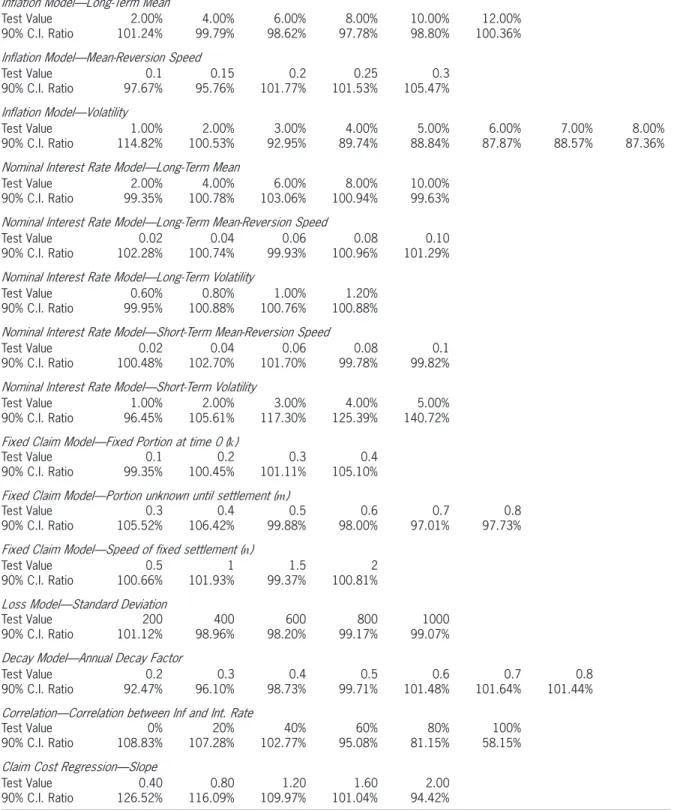
Table 2-A. Sensitivity analysis results

Inflation Model—Long-Term Mean

Test Value 2.00% 4.00% 6.00% 8.00% 10.00% 12.00% 90% C.I. Ratio 101.24% 99.79% 98.62% 97.78% 98.80% 100.36%

Inflation Model—Mean-Reversion Speed

Test Value 0.1 0.15 0.2 0.25 0.3 90% C.I. Ratio 97.67% 95.76% 101.77% 101.53% 105.47%

Inflation Model—Volatility

Test Value 1.00% 2.00% 3.00% 4.00% 5.00% 6.00% 7.00% 8.00% 90% C.I. Ratio 114.82% 100.53% 92.95% 89.74% 88.84% 87.87% 88.57% 87.36%

Nominal Interest Rate Model—Long-Term Mean

Test Value 2.00% 4.00% 6.00% 8.00% 10.00% 90% C.I. Ratio 99.35% 100.78% 103.06% 100.94% 99.63%

Nominal Interest Rate Model—Long-Term Mean-Reversion Speed

Test Value 0.02 0.04 0.06 0.08 0.10 90% C.I. Ratio 102.28% 100.74% 99.93% 100.96% 101.29%

Nominal Interest Rate Model—Long-Term Volatility

Test Value 0.60% 0.80% 1.00% 1.20% 90% C.I. Ratio 99.95% 100.88% 100.76% 100.88%

Nominal Interest Rate Model—Short-Term Mean-Reversion Speed

Test Value 0.02 0.04 0.06 0.08 0.1 90% C.I. Ratio 100.48% 102.70% 101.70% 99.78% 99.82%

Nominal Interest Rate Model—Short-Term Volatility

Test Value 1.00% 2.00% 3.00% 4.00% 5.00% 90% C.I. Ratio 96.45% 105.61% 117.30% 125.39% 140.72%

Fixed Claim Model—Fixed Portion at time 0 (k)

Test Value 0.1 0.2 0.3 0.4 90% C.I. Ratio 99.35% 100.45% 101.11% 105.10%

Fixed Claim Model—Portion unknown until settlement (m)

Test Value 0.3 0.4 0.5 0.6 0.7 0.8 90% C.I. Ratio 105.52% 106.42% 99.88% 98.00% 97.01% 97.73%

Fixed Claim Model—Speed of fixed settlement (n)

Test Value 0.5 1 1.5 2 90% C.I. Ratio 100.66% 101.93% 99.37% 100.81%

Loss Model—Standard Deviation

Test Value 200 400 600 800 1000 90% C.I. Ratio 101.12% 98.96% 98.20% 99.17% 99.07%

Decay Model—Annual Decay Factor

Test Value 0.2 0.3 0.4 0.5 0.6 0.7 0.8 90% C.I. Ratio 92.47% 96.10% 98.73% 99.71% 101.48% 101.64% 101.44%

Correlation—Correlation between Inf and Int. Rate

Test Value 0% 20% 40% 60% 80% 100% 90% C.I. Ratio 108.83% 107.28% 102.77% 95.08% 81.15% 58.15%

Claim Cost Regression—Slope

Test Value 0.40 0.80 1.20 1.60 2.00 90% C.I. Ratio 126.52% 116.09% 109.97% 101.04% 94.42%

that is not fixed in value until the claim is settled (m), the lower the confidence interval ratio. The rate of fixing a claim’s value (asnincreases) had no consistent effect on the confidence interval ratio.

inter-val ratio. Changing the decay factor represent-ing what portion of unsettled claims were set-tled each year had a slight impact on the confi-dence interval range; a higher decay factor led to a higher confidence interval range. Changing the correlation between the inflation rate and the nominal interest rate from 0% to 100% had a sig-nificant impact on the confidence interval ratio. The higher the correlation, the lower the confi-dence interval ratio. Increasing the slope in the claim cost regression formula over the range of 0.4 to 2.0 also decreased the confidence interval ratio.