Another Look at the Perceptron

(1)

1

Mathematical and Software Engineering, vol. 5, no. 1 (2019), 1-8. Varεpsilon Ltd, http://varepsilon.com

Another Look at the Perceptron

Ertan Geldiev

1

and Nayden Nenkov

2

1

Varna University of Management, Varna, Bulgaria email: [email protected]

2

Konstantin Preslavsky University of Shumen, Shumen, Bulgaria, email: [email protected]

Abstract

The article explores a method for classifying elements of linearly separable sets using the Perceptron algorithm and implemented with Python.Experimented in two-dimensional space with the following sets: linearly separated, linearly separated by elements close to the line and merging elements into one another. The optimal weights of the linear predictive function weights are searched using a Stochastic Gradient Descent. The purpose is to find the weights with reference to error of the minimum predictive function minus the real value of the class, following the changing weights of the moving of the gradient.

The aim of the article is to show an opportunity to solve classification problem using a single neural network. Because the classification method is limited to linearly divisible sets, and often we do not know whether the sets are such previously a variant of the perceptron algorithm is offered which, in case of impossibility of further detection of more optimal weights, stops automatically and possibly use other classification algorithms for a more accurate classification.

Keywords: perceptron, linear separable classification, stochastic gradient descent, neural networks

1 Introduction

Two sets X1 and X2 belonging to the n multi-dimensional space Rn can be assumed to be linearly separable if only one hyperplane exist with a smaller dimension than Rn is capable of dividing them. In the two-dimensional space this hyperplane contains many straight lines.

The methods for testing linearly separable sets [1] are: - based on linear programming;

- based on computational geometry; - based on neural networks

- based on quadratic programming; - The Fisher linear discriminant method; - Others.

In the study, we are only pursuing the machine training of the neural network consisting of a single Perceptron. With his rule for Perceptron, Rosenblatt [1] offers an algorithm that automatically learns the optimum weights, which are then multiplied by the input characteristics to decide whether a neuron is triggered. In the context of observed training and classification, such an algorithm could be used to predict whether a sample belongs to one or another class. Perceptron is a binary classification algorithm that uses a linear predictive function

(2)

2

2 Proposed Algorithm

In our example, we assume that the prediction class gets values 1 and 0 (for ease), and we also have only two input variables x1 and x2.

In the linear activation function, which is also the predictive function f(x1,x2) = w1*x1 + w2*x2 + b

x1 and x2 are the input variables, w1 and w2 are the weights we are looking for, and b is a slope that is also being searched.

f(x1,x2) = 1 , when w1*x1 + w2*x2 + b >= 0 f(x1,x2) = 0 , when w1*x1 + w2*x2 + b < 0

Finding of the weights is done through the training of the Perceptron. Following is the algorithm - Training of Perceptron:

1. Initializing the all weights w with zero

2. Entry through training data. For each iteration, the instance is classified: a) if the prediction of the output i.e. the class is correct, no action is taken b) if prediction is wrong, modifying weights with a modifying rule is necessary

w(i) = w(i) + learning_rate * (f(x(i))_expected - f(x(i))_predicted) * x(i)

3. Step 2 is performed until the perceptron has correctly classified each instance or has reached the maximum number of times set

Algorithm implementation situations

If the dataset elements are not a linearly separable the classifier will always return an error, or if the weights are not found exactly, the error will be different from zero

Loss = (f(x)_expected – f(x)_predicted)

When we have a mistake, we have options for stopping the algorithm:

a) It is necessary to set a stop criterion when the algorithm stops making upgrades or cycles indefinitely.

b) Set the final number of iterations or epochs (The number of times the training data will be run while updating the weight).

Learning Rate (Learning - Rate Typically a constant between 0.0 and 1.0 [4]) - Opportunity options. Used to limit the amount to be adjusted at each update.

а) with a small LR algorithm will be slow because updating will not make much progress. b) with a large LR, the algorithm will be slow because updates will "exceed", ie skip the local minimum.

Execution

The search algorithm for w1, w2, and b weights is realized using a ready-made implementation of Python software [3] with slight changes to the code associated with reading our datasets.

(3)

3

Data sets have three attributes X1, X2 and CLASS (0,1) and contain about 1000 lines.

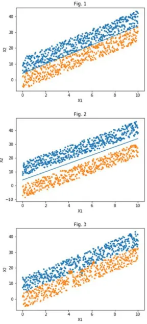
The linear used to divide the sets can be described by the equation: x2 = 3*x1 + 4, by generating points on both sides uses rand (1) from Python with a positive and negative sign on the upper right equation

Results

(4)

4

Table1: Data set results Learning

Rate

Close-up sets – Fig.1 [w1,w2, b ]

Multitudes are some distance apart– Fig.2 [w1,w2, b ]

Spill-over sets– Fig.3 [w1,w2, b ]

lrate=0.000 >epoch=999, error=501.00 [0.0, 0.0, 0.0]

>epoch=9, error=501.00 [0.0, 0.0, 0.0]

lrate=0.010 >epoch=9999, error=7.00

[-47.54, -39.60, 12.88]

>epoch=4, error=0.00 [-0.20, -0.45, 0.14]

>epoch=9999, error=34.00 [-14.50, -10.95, 3.65] lrate=0.010 >epoch=19998, error=6.000

>epoch=19999, error=7.000 [-61.49, -51.00, 16.59]

>epoch=19999, error=40.000

[-14.49, -10.95, 3.69] lrate=0.100 >epoch=9999, error=7.000

[-475.40, -396.01, 128.82]

>epoch=1, error=0.000 [-2.00, -4.56, 1.29]

[-950.80, -792.02, 257.65

>epoch=2, error=0.000 [-4.00, -9.12, 2.59]

[-1901.60, -1584.05, 515.29]

>epoch=2, error=0.000 [-8.00, -18.24, 5.18]

[-3327.80, -2772.08, 901.77]

>epoch=2, error=0.000 [-13.99, -31.92, 9.07]

>epoch=9999, error=34.000 [-1015.00,-766.63, 255.43] lrate=0.900 >epoch=9999, error=7.000

[-4278.60, -3564.10 1159.42]

>epoch=2, error=0.000 [-18.0, -41.04, 11.66]

>epoch=9999, lrate=0.900, error=34.000

[-1305.00, -985.66, 328.41] lrate=1.000 >epoch=9999, error=7.000

[-4754.0, -3960.12, 1288.24]

>epoch=2, error=0.000 [-20.0, -45.60, 12.96]

[-9508.0, -7920.24, 2576.48]

>epoch=2, error=0.000 [-40.0, -91.20, 25.92]

[-14262.0, -11880.36, 3864.72]

>epoch=2, error=0.000 [-60.0, -136.8, 38.88]

>epoch=9999, error=34.000 [-4350.0, -3285.54, 1094.70]

(5)

5

In Figures 6 and 7, at spaced sets, the perceptron is well behaved, and after two epochs it reaches zero and the algorithm has to be stopped.

(6)

6

The steps for implementing a constraint algorithm are as follows: 1. Initially set lrate, epoch, sum_error_stop, n_oscillations. 2. The weights are searched using the Perceptron algorithm.

3. If (sum_error <sum_error_stop) n_oscillations times then the algorithm should stop before reaching the total number of epochs.

4. Print of calculated weights and error.

When running the algorithm with the limits lrate = 0.01, epoch = 20000, sum_error_stop = 8, n_oscillations = 1000 is obtained:

>epoch=1444, lrate=0.010, error=7.000

[-22.89000000000078, -19.828199999997445, 6.428819999998381] In datasheet Table 1 in Fig. 1, we have the data:

lrate=0.010

>epoch=19998, error=6.000 >epoch=19999, error=7.000 [-61.49, -51.00, 16.59]

If we set the rate = 0.01, epoch = 20000, sum_error_stop = 8, n_oscillations = 2000 we get: >epoch=1444, lrate=0.010, error=7.000

[-22.89000000000078, -19.828199999997445, 6.428819999998381]

Because in the Perceptron algorithm with constraints we added a comparator operator that is executed 1000 times and loads the algorithm, then the result is visible for about 1400 epochs and not with a consecutive increase of the epochs to 20000 in the example.

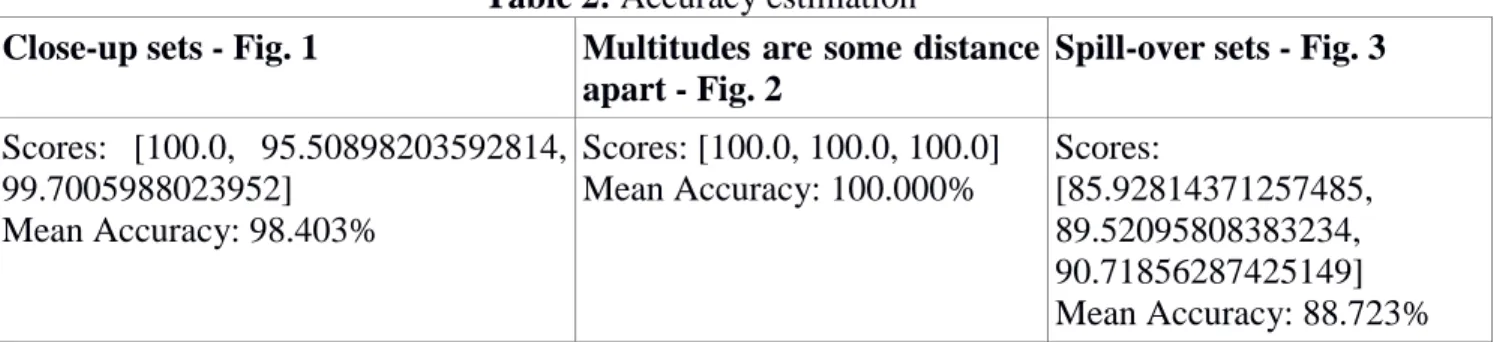
If we replace the resulting weights in one of the columns in a prediction program, the classification we will be able to classify the data. Using cross validation [5], we estimate accuracy in Table 2.

Table 2: Accuracy estimation

Close-up sets - Fig. 1 Multitudes are some distance apart - Fig. 2

Spill-over sets - Fig. 3

Scores: [100.0, 95.50898203592814, 99.7005988023952]

Mean Accuracy: 98.403%

Scores: [100.0, 100.0, 100.0] Mean Accuracy: 100.000%

Scores:

[85.92814371257485, 89.52095808383234, 90.71856287425149] Mean Accuracy: 88.723%

3 Conclusions

From the experiments, it can be seen that the finding of weights by means of a stochastic gradient also works with slightly fused elements, i. incomplete linear separation. The Perceptron is a good algorithm for predicting and classifying only when the output data is linearly separable. Modifying it with external limiters saves processor time.

(7)

7

References

[1] Rosenblatt, F. (1957) The perceptron, a perceiving and recognizing automaton Project Para. Cornell Aeronautical Laboratory

[2] Elizondo, D. (2006) The linear separability problem: Some testing methods. IEEE Transactions on neural networks, 17(2), 330-344.

[3] Brownlee, J. (2016) How To Implement The Perceptron Algorithm From Scratch In Python,

In Code Machine Learning Algorithms From Scratch -

https://machinelearningmastery.com/implement-perceptron-algorithm-scratch-python/

[4] Raschka, S., Mirjalili, V. (2017) Python machine learning. Packt Publishing Ltd.

[5] Moore, A. W., & Lee, M. S. (1994) Efficient algorithms for minimizing cross validation error. In Machine Learning Proceedings 1994 (pp. 190-198). Morgan Kaufmann.

Copyright © 2019 Ertan Geldiev and Nayden Nenkov. This is an open access article distributed under the Creative Commons Attribution License, which permits unrestricted use, distribution, and reproduction in any medium, provided the original work is properly cited.

Python source code:

from csv import reader # Load a CSV file def load_csv(filename):

dataset = list()

with open(filename, 'r') as file: csv_reader = reader(file) for row in csv_reader:

if not row: continue dataset.append(row) return dataset

# load and prepare data filename = 'close_points.csv' dataset = load_csv(filename)

#print(type(dataset)) #print (len(dataset)) #print (dataset[0]) #print (dataset[1]) #print (dataset[2])

import matplotlib.pyplot as plt import array as w_arr

import numpy as np

def predict(row, weights): activation = weights[0] for i in range(len(row)-1):

activation += weights[i + 1] * float(row[i]) return 1.0 if activation >= 0.0 else 0.0

# Estimate Perceptron weights using stochastic gradient descent def train_weights(train, l_rate, n_epoch,sum_error_stop): w_arr=[]

weights = [0.0 for i in range(len(train[0]))] for epoch in range(n_epoch):

sum_error = 0.0 j=0

(8)

8

# print("The algorithm stops due to set limiters!") # break

#w_arr = w_arr.append(2) for row in train:

prediction = predict(row, weights)

error = float(row[-1]) - float(prediction) sum_error += error**2

weights[0] = weights[0] + l_rate * error for i in range(len(row)-1):

weights[i + 1] = weights[i + 1] + l_rate * error * float(row[i]) w_arr.append(sum_error)

w_arr.append(epoch)

if sum_error < sum_error_stop and j <= 2000: print (sum_error , '<' , sum_error_stop)

print('>epoch=%d, lrate=%.3f, error=%.3f' % (epoch, l_rate, sum_error)) j=j+1

return weights break

print('>epoch=%d, lrate=%.3f, error=%.3f' % (epoch, l_rate, sum_error)) #w_arr = w_arr.append(1)

#print(w_arr) print(sum_error) return weights,w_arr

l_rate = 0.01 n_epoch = 20000 rezult_array=[] sum_error_stop = 8

weights = train_weights(dataset, l_rate, n_epoch, sum_error_stop) print(weights)

#print (rezult_array)

# printing the list using loop #for x in range(len(rezult_array)): # print (rezult_array[x],)

#plt.savefig('Fig_1.png') #

# counter = 0