ANALYSES OFPHYSICIANLABORSUPPLYDYNAMICS AND ITSEFFECT ONPATIENTWELFARE
Jing Teresa Zhou
A dissertation submitted to the faculty at the University of North Carolina at Chapel Hill in par-tial fulfillment of the requirements for the degree of Doctor of Philosophy in the Department of
Economics.
Chapel Hill 2018
Approved by:
Donna Gilleskie
Luca Flabbi
Jane Fruehwirth
David Guilkey
c
2018
ABSTRACT
Jing Teresa Zhou: Analyses of Physician Labor Supply Dynamics and its Effect on Patient Welfare (Under the direction of Donna Gilleskie)
My dissertation focuses on the supply side of health and labor economics in order to inform policymakers who seek to address physician shortages and thus improve patient welfare in the United States.
The first chapter evaluates the determinants of physician geographic and professional movement within North Carolina (NC) using a dynamic discrete choice model designed to analyze labor supply behaviors of indi-viduals over time. I jointly model the initial specialty, activity, location, facility, and hours of direct patient care of all physicians in NC from 2003 to 2012 using a full information maximum likelihood estimation approach that allows for correlation of unobserved determinants. Using the parameter estimates from the dynamic model, I simulate several policy interventions aimed to attract and retain physicians in rural and underserved areas. I find that loan forgiveness policies are less effective at decreasing the probability of movement and increasing retention in the same rural county than an increase in the reimbursement rate. An increase in midlevel practi-tioners decreases retention in rural areas and increases the likelihood of a physician becoming inactive, while an increase in registered nurses in rural areas significantly increases physician retention.
To my parents, Dr. Hong Zhou and Ms. Ning Liu, whose love, selfless support and passion for learning laid the foundation for the discipline and application necessary to complete this work.
ACKNOWLEDGMENTS
I would like to thank my advisor, Donna Gilleskie, for guiding and supporting me over the years at the University of North Carolina at Chapel Hill. You have set an example of excellence as a researcher, mentor, instructor, and role model for me. I am forever indebted to all the guidance you have given me and I hope I can follow in your footsteps in becoming a better person each day.
I would like to thank my thesis committee members, Luca Flabbi, Jane Fruehwirth, David Guilkey, and He-len Tauchen, for all their valuable guidance through this process. The discussion, interchange of ideas, and feedback have been absolutely invaluable.
TABLE OF CONTENTS
1 Introduction . . . 1
2 The Doctor is In/Out: Determinants of Physician Labor Supply Dynamics . . . 4
2.1 Introduction . . . 4
2.2 Literature Review . . . 6
2.3 Data and Summary Statistics . . . 9
2.3.1 Physician Level Panel Data . . . 9
2.3.2 Specialty, Experience, and Demographics . . . 16
2.3.3 Salary Data . . . 20
2.3.4 County-Level Data . . . 21
2.4 Theoretical Motivation . . . 24
2.5 Empirical Framework . . . 26
2.5.1 Per-Period Employment Behaviors . . . 27
2.5.2 Initial Conditions . . . 30
2.5.3 Likelihood Function . . . 32
2.5.4 Identification . . . 32
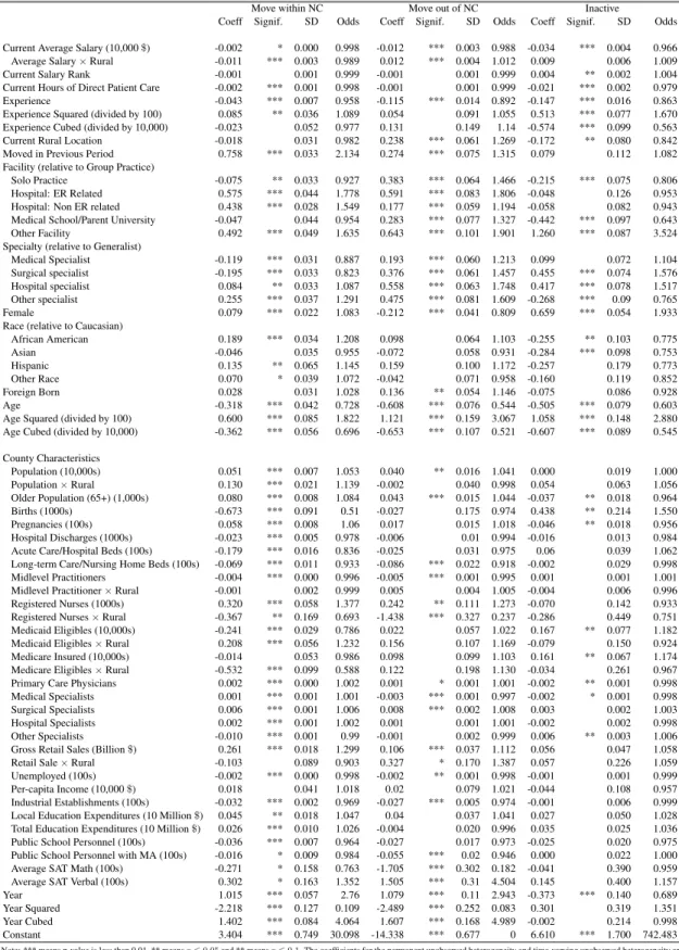
2.6 Estimation Results . . . 33
2.6.1 Model Fit . . . 34
2.6.2 Results from the Dynamic Multiple-equation Model . . . 35
2.6.3 Policy Experiments . . . 38
2.7 Conclusion . . . 46
3.1 Introduction . . . 48
3.2 Literature Review . . . 50
3.3 Existing Policies . . . 52
3.4 Data and Summary Statistics . . . 54
3.4.1 Inpatient Hospital Discharge Data (Patient-Level Data) . . . 55
3.4.2 Physician Licensure Database (Physician-Level Data) . . . 56
3.4.3 Log Into North Carolina (County-Level Data) . . . 57
3.5 Theoretical Model . . . 57
3.5.1 Individual’s Problem . . . 57
3.5.2 PCP Problem . . . 59
3.6 Empirical Model . . . 60
3.6.1 HPSA designation and its Significance . . . 60
3.6.2 Fuzzy Regression Discontinuity Design . . . 61
3.7 Results . . . 63
3.8 Conclusion . . . 65
A Appendix for Chapter 2: Determinants of Physician Labor Supply Dynamics . . . 66
A.1 Results from Conditional Multinomial Logit . . . 66
A.2 Location and Rurality Construction . . . 68
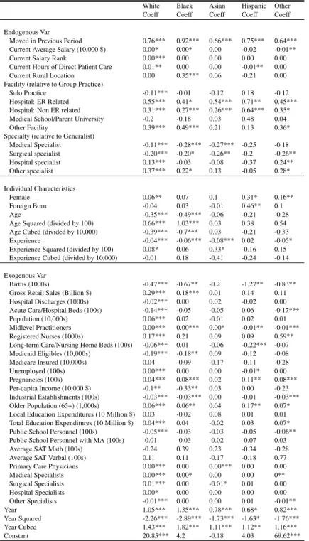
A.3 Estimation Results by Race . . . 70
A.4 Additional Estimation Results . . . 78
A.5 Results from Policy Experiment Comparing Between Zipcode and County Level Shocks . . . . 82
B Appendix for Chapter 3: Identifying the Effect of Physician Supply on Ambulatory Care Sensi-tive Condition Admissions . . . 85
B.1 Tables and Figures . . . 85
WORKS CITED FOR CHAPTER 2 . . . 102
CHAPTER 1
INTRODUCTION
The Gross Domestic Product (GDP) of the United States in 2014 was around 17.4 trillion dollars, almost 7 trillion dollars more than the second largest economy. Perhaps even more mind-boggling is the fact that one out of every six dollars spent in the US that year is spent on health care (i.e., 17 percent of GDP went toward national health expenditures, NHE, compared to the 10 percent world average), in the form of physician office visits, surgeries, medicines, and new investments in medical research.1 In the US, twenty percent of total NHE constitutes physician and clinical services, which is the second largest category after hospital care (32%).2 In addition to its substantial monetary cost, adequate physician presence is essential to patient welfare. However, undersupply of physicians is a pressing health issue in the US and around the world. Concern exists among the public that a continuing physician shortage will drive up medical care costs, increase waiting times, shorten office visits and, generally, decrease overall patient welfare.3 A significant amount of research has shown that, instead of an aggregate shortage, there is a maldistribution of physicians both geographically and by specialty in the US. Existing physician supply models challenge our ability to understand incentives, with the objective of promoting equity of access, since they do not consider in detail the physician and location characteristics that affect physician location decisions. Multiple programs (federal and state) have been created to increase physician supply to meet physician shortages. However, these programs have had limited success at maintaining physician presence in underserved areas.
My dissertation addresses the supply side of the health care market using both economic theory and empirical strategies in the form of two stand-alone papers in the following chapters. My first paper (Chapter 2) focuses on building a holistic physician supply model captures the employment behavior of physicians in the US. Existing physician supply models challenge our ability to understand incentives, with the objective of promoting equity of access, since they do not consider in detail the physician and location characteristics that affect physician
1
Health expenditure, total (% of GDP): World Health Organization Global Health Expenditure database, The World Bank.
2
National Health Expenditure Data, 2014: Centers for Medicare & Medicaid Services, Office of the Actuary, National Health Statistics Group.
location decisions. My paper evaluates the determinants of physician geographic and professional movement within North Carolina (NC) using dynamic empirical models designed to analyze the behavior of individuals over time. I jointly model specialty, practice location, facility type, and hours worked of all physicians in NC from 2003-2012. I also study the determinants of physician movement within NC by race and ethnicity, which has not been studied in detail. In order to address these questions, I collected physician data from the NC medical board, which tracks all physician movement across NC. I obtained the physician licensures of all board-certified physicians in NC from 2003-2012 and used the information to construct a database that includes physician demographics, specialty, location of practice, facility type, and hours worked for each year an individual physician practices in NC over this period. I have also merged the physician-level information with county-level information from Log into NC (LINC), and with constructed salary variables from the Hospital and Healthcare Compensation Service (HHCS) and NC Occupational Employment Statistics (OES).
Using the model I built, my research informs policies aimed to attract more physicians to underserved communities and to maintain their presence in order to achieve equity of health care access in the US. However, in reality, there has not been an amelioration of this problem due to the low retention of physicians in underserved areas. In this paper, I find programs that forgive medical school debt if a physician serves in a rural area is less effective at retaining physicians in rural areas than an increase in reimbursement rates, which increases the physicians salary. In another words, loan forgiveness programs are a short-term solution to a long-term problem. I also find a change in other medical care providers or support staff also affects physician behavior, where mid-level practitioners (i.e., physician assistants, advance nurse practitioners) decrease retention and increase physician transition to inactivity-and are thus a substitute for physicians- while an increase in Registered Nurses (or RNs), a complement to physicians, significantly increases retention in rural areas.
than waiting for acute manifestations of these ailments that results in hospital admissions.
CHAPTER 2
THE DOCTOR IS IN/OUT: DETERMINANTS OF PHYSICIAN LABOR SUPPLY DYNAMICS
2.1 Introduction
Two concerns about physician labor supply dominate the academic literature and the popular press: short-age and maldistribution. The American Medical Association (AMA) contends that their data, used by the US Department of Health and Human Services (USDHHS) to calibrate physician workforce models, uncover sig-nificant current and anticipated shortages.1 Other researchers (Zurn, 2004; Dussualt, 2006; and Dorsey, 2011) argue that there exists a maldistribution of physicians both geographically and by specialty, which leads to a shortage of certain types of doctors in some areas and a surplus in other areas. Indeed, a frequent observation about physicians is the clustering of specialists in metropolitan areas and a shortage of physicians in rural areas. Some argue that an important contributor to this uneven distribution is financial barriers that prevent individuals who would be the most likely to serve in primary care and in underserved areas from entering the profession (Vaughn, et al., 2010; Dorsey et al., 2011). Others emphasize that physicians tend to be attracted to areas with complementary staff in order to practice effectively (Stange, 2003; Roblin et al., 2004; MGMA, 2016). Others argue that current health care system regulations that require a substantial amount of documentation by physi-cians have reduced the time available for direct patient care and could potentially increase burn out (Christino, et al., 2017). Efforts to mitigate these concerns require an understanding of determinants of physician labor supply decisions regarding specialty, geographic location, facility type, hours worked and continued practice over one’s career.
Current leading models of physician supply, developed by the AMA, USDHHS and American Association of Medical Colleges (AAMC), aggregate physician behavior to the national or state level, while ignoring individual preferences shaped by gender, race, and experience as well as within-state variations in physician demand, supply conditions, and location amenities. A recently-developed interactive tool, the FutureDoc Forecast Tool,
1
improves upon the three models by allowing some physician mobility and disaggregation to the county level.2 The forecasting model, which uses inventory projections from historical data on separation and arrival rates, does not attempt to explain what drives observed physician employment behaviors.
I formulate and estimate a dynamic model of physician behaviors that includes initial specialty, activity (whether or not to remain active), location, facility, and hours of direct patient care. I use the population of licensed physicians in North Carolina (NC) over 10 years (2003-2012) to explore the underlying factors that ex-plain the professional behaviors of physicians. An economic model of mobility decision-making motivates a set of estimable, correlated, and dynamic labor supply equations whose probabilities or densities form the likelihood of observed physician employment outcomes in the research sample. In addition to individual-level explanatory variables such as gender, race, and age, time-varying county-level characteristics that capture location-specific quality of life, number of physician substitutes or complements (i.e., advanced nurse practitioners, physician as-sistants and registered nurses) and potential demand shifters help identify endogenous individual behaviors over time. The endogenous histories of behaviors (i.e., work experience, lagged hours worked, facility choices, etc.) also explain current behaviors. I use the estimated data-generating process to simulate the effects of potential policies likely to affect physician migration patterns such as loan forgiveness, increases in service reimbursement rates, midlevel practitioner or registered nurse growth, and changes in Medicare/Medicaid coverage.
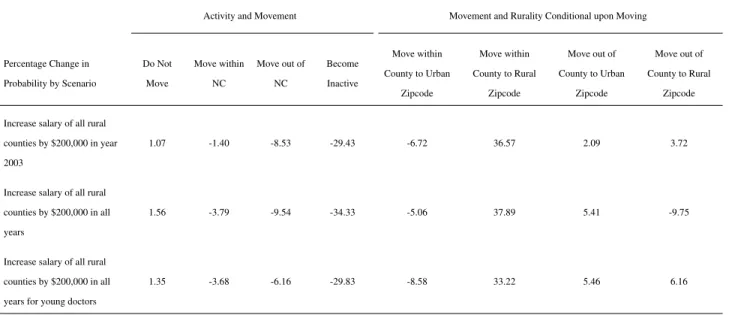
To simulate the existing loan forgiveness programs that aim to attract and retain physicians in rural areas, I allow for a lump sum wage increase of $200,000 for all rural physicians in one year. Although the simulated policy is the most generous version of the loan forgiveness program, I find that it does not significantly decrease the average likelihood of movement nor does it decrease the probability of moving one or two years of service in a rural area (i.e., retention). However, an increase in the reimbursement rate in rural counties via a proportional increase in average salary has the potential to increase physician retention in rural areas. A 5-percent increase in rural county salaries decreases the probability of moving after one year by 11.7 percent and moving after two years by 6.7 percent. Male physicians are more responsive to the policy change than female physicians and, for both groups, there is a decreasing marginal return to a larger increase (10 or 20 percent) in salary. Other policies that impact physician movement and retention involve changing the composition of other medical care professionals. A 5-percent increase in midlevel practitioners in rural counties increases the probability of moving after one or two years by 15.7 percent and 8.3 percent, respectively. The policy also significantly increases the likelihood of a physician exiting the labor force by becoming inactive. A 5-percent increase in
2
RNs in rural counties significantly decrease the probability of leaving after one year and two years of service by 13.8 percent and 2.7 percent, respectively. These findings offer a new understanding of the effectiveness of policies that attempt to change physician behavior and increase retention in rural and underserved areas.
In the next section, I review the relevant literature regarding physician labor supply. Section 3 describes data from the North Carolina Board of Medicine, Log into NC and the Physician Compensation Survey and details construction of the research sample. Section 4 presents a theoretical discrete choice framework that motivates the empirical model detailed in Section 5. Results are presented and discussed in Section 6. Section 7 concludes and provides a discussion of future research.
2.2 Literature Review
Leading physician supply models in the policy research literature simplify physician employment behavior by ignoring many physician characteristics such as race and experience as well as detailed location charac-teristics. Most of the existing models also aggregate physician labor supply to the national or state level by estimating the historical probability of physician inflow and outflow, while disregarding physician preferences and within-state variations. For example, the most commonly used Physician Supply Model (PSM) developed by the AMA and USDHHS is an inventory model that tracks the supply of physicians by age, gender, country of medical education, type of degree and medical specialty. The model uses historical data to determine the prob-ability that physicians will remain active from year to year and the annual number of hours worked in patient care at the national level. The model takes the number of physicians at timet(starting with the base year 2000), adds in new additions to the physician labor force (i.e., new US medical graduates and international medical graduates) and subtracts attrition each year (due to retirement, death, and disability), arriving at the physician supply for yeart+ 1. The extrapolation of the supply of physicians and hours worked is assumed to be linear in the probability of retirement or death, the probability of being accepted into medical school, graduation from medical school, and other probabilities based on age, gender and specialty. The PSM does not address the heavy presence of physicians in metropolitan areas and severe shortages in rural or poor areas, does not consider move-ment at the state or county levels, and does not include other individual characteristics such as race or exogenous location-specific amenities or medical market characteristics.
worked over all age or gender groups. Similar results are found for US physician supply (Weisman et al.,1980; Fossett, et al., 1990). Female physicians tend to have higher retirement rates and to work fewer hours in direct patient care, and female physicians are concentrated in pediatrics and psychiatry and are underrepresented in general surgery and other medical subspecialties (Kletke et al., 1990). Although there is a growing representation of female physicians in the labor force, the supply of physicians continues to reflect differential selection of specialty by gender.
The economics literature on labor mobility highlights the role of individual preferences for location char-acteristics. Although higher (lower) wages and better (worse) economic opportunities are often credited as the major factors that induce general migration into (out of) an area (Muth, 1971; Olvey, 1972; Greenwood, 1985; Partridge and Rickman, 2006), studies have shown the importance of location-specific amenities and positive quality of life measures as drivers of general migration (Cushing, 1987; McGranahan, 1999; Green, 2001; Deller et al., 2001; Cebula and Payne, 2005; Gunderson and Ng, 2006). In seminal work by Roback (1982), the author claims that better amenities would drive down wages and drive up rents, but individuals would rather trade off higher wages and pay higher rents to live in those communities. Building on the same principle, Blanchflower and Oswald (1994, 1995) incorporate Smith’s (1985) compensating differential and extend the Roback model in the presence of unemployment. These papers assume free mobility of labor because when migration is costly, workers are more likely to view the decision to migrate as an investment. However, Clark et al. (2003) find that when there are both pecuniary and psychic costs associated with moving, households are generally more responsive to undercompensation between income and location characteristics than overcompensation (i.e., the household perceives a higher opportunity cost of not moving than moving, conditional on the compensation level at the destination and at the origin being the same). These theories tell us that, for an agent with a high wage, there exists a high marginal cost of living in a location with relatively low amenities because, for that person, the marginal benefit of having better amenities is high. Therefore, the agent is more likely to move to an area with relatively higher amenities and lower wages.
In addition to the amenity and wage trade-off literature, a number of studies find that high-income individuals have small or negligible labor supply elasticity with regard to earnings (Pencavel, 1986; Roed and Strom, 2002). Showalter and Thurston (1997) extend their research on white-collar professional labor market decisions to US physicians and focus on tax effects. They find that self-employed physicians are sensitive to marginal tax rate changes, but the effect is small and insignificant for employed physicians. Since physicians are some of the most highly paid professionals in the US,3the literature hypothesizes that they are more likely to accept a decrease in
income for better amenities and the earnings elasticity of labor supply is small.
Recent empirical economic studies use dynamic panel data models and structural discrete choice models to study labor supply (Rizzo and Blumental, 1994; Scott, 2000; Saether, 2005; Baltagi et al., 2005; Cheng et al., 2013; Wang and Sweetman, 2013; Kalb et al., 2015; Andreassen et al., 2013; Broadway et al., 2017). Rizzo and Blumental (1994) evaluate the effects of both income and non-labor income on US physician labor supply among self-employed physicians. They find that the income effect of an earnings change for male physicians is negative. Controlling for the income effect, a one percent increase in wages leads to a 0.49 increase in labor supply. Using Norwegian hospital data between 1993-1997, Baltigi et al. (2005) find labor supply elasticities are around 0.3, but they do not control for physicians heterogeneity across specialties. Saether (2005) uses a static random utility labor supply model and finds that a wage increase causes a small response in total hours and reallocation of hours within the sectors with increased wages. Broadway et al. (2017) estimate a structural, discrete choice model of labor supply and after-hour care (AHC) in a sample of Australian general practitioners. They find that physicians are more likely to increase after-hour care if their daytime-weekday hourly earnings increases, but the effect is very small. Yet, in another setting, hourly wage increases actually reduce the probability of providing AHC, especially among male physicians. The results lead them to conclude that wage increases appear to be, at best, relatively ineffective in incentivizing increased provision of AHC and may even prove harmful if incentives are not well targeted. None of these studies explicitly consider each of the relevant professional decisions of physicians over time nor do they differentiate behavior by race, gender, facility type, or specialty. In addition, they are unable to measure the short- and long-run effects of potential policies that may dynamically impact behaviors through location and facility changes.
My work contributes to the physician labor supply literature by estimating a dynamic model of physician employment behavior (i.e., initial specialty, annual location, facility type, and hours of direct patient care) that accounts for physician preference shifters (i.e., gender, race, age, experience), location-specific amenities, and medical care market characteristics. The ability to separately identify the importance of these factors and to quantify the heterogeneous impact of these factors on physician employment decisions allows us to evaluate the impact of financial incentives that may vary by individual characteristics. Using the estimated parameters of the dynamic data generating process, I simulate the behavior of physicians over time under different policy scenarios.
2.3 Data and Summary Statistics
Before presenting an economic model of location decisions and professional behavior of physicians, I begin by describing the data that are available. The specific structures of these data inform and dictate the empirical modeling in important ways. The first section details three sources of data, describes variable construction, and summarizes the variables used in analyses. The second section describes the constructed annual income data and the last section describes the county-level medical care market and local amenity characteristics.
2.3.1 Physician Level Panel Data
The North Carolina Physician Licensure Database from the North Carolina Medical Board provides annual physician-level data from 2003 to 2012. The data are collected and released by the North Carolina Health Professions Data System (HPDS). The database tracks the universe of physician applications for NC medical licenses, which must be renewed annually. It provides a comprehensive view of the physician labor force in the state and allows a researcher to track the movement of all physicians within the state across time.
Prior to May 2009, the state allowed two methods for annual license renewal: paper and electronic. Com-plicated to process and prone to mistakes, paper applications have been phased out in favor of an electronic renewal process on the NC Medical Board website. Because medical licenses are time delimited, the Board sends a renewal notice two months before each physician’s deadline (dated as his/her birthday). On average, the electronic renewal process takes about 15 minutes because the information regarding education history, de-mographics, and work history often remains unchanged. If a physician changed location of practice, facility type, or specialty, they must update this information. Many physicians also provide updates when they decide to become inactive, by indicating retirement or other reasons. Inactive physicians that annually update their status can avoid a time-consuming reinstatement process should they decide to return to practice.4
If a physician fails to renew the license on time, a grace period of 30 days is provided and the physician is charged an additional late fee. If renewal is not completed during the grace period, the license is placed on inactive status and it is illegal to practice medicine or surgery, write prescriptions or administer prescription drugs in NC under any circumstances. If the inactivity period is less than one year, it is necessary to pay an additional fee and undergo a background check to reactivate the license.
However, if there has been an interruption in the continuous, clinical practice of medicine greater than two years, the applicant may have to reestablish his or her competence to practice medicine safely to the Board’s
4Among physicians who become inactive by notifying the board, rather than failure to renew, the four most common reasons are:
satisfaction, in accord with GS 90-14 (11a). The reinstatement procedure might entail, and is not limited to, full-scale assessments, engagement in formal training programs, supervised practice arrangements, formal testing (Board Examination), or other proofs of competence. The Board is much more likely to require a physician who has not maintained annual notification of reason for inactivity to undergo these competency procedures.5 Such decisions are made on a case by case basis.
After a physician submits his/her application, the information is processed and updated in HPDS. Basic information in the database includes an ID number to identify the physician through time (not the board license number), gender, race, age, medical school, internship, residency, location of practice, facility type, and practice specialty.
The data obtained from the Medical Board include 43,765 uniquely-identified physicians or a total of 293,835 person years over the period 2003-2012. These person-year observations include all instances where physicians maintained either active or inactive status in NC; 5,427 physicians are never active in NC and 5,339 physicians appear only once in the sample. I restrict the research sample to the longest spell of continued com-munication with the Board for each physician. I do not include multiple spells within the observation period of the data because I do not observe a physician’s activities between spells and therefore cannot construct relevant variables that explain re-entry into the NC physician labor force. Prior to selection based on the longest spells, person-year observations for which location, facility type or hours worked is missing and cannot be intelligently imputed are considered a break in a spell; 2,518 physicians are missing employment location that cannot be filled in and 573 are missing facility or specialty. The research sample also includes physicians with at least two years of observation in order to model location transitions. With these necessary removals, my research sample contains 29,908 uniquely-identified physicians who contribute two to 10 years of observed practice behaviors, for a total of 187,402 person-year observations. Conditional on being active in NC and having renewed their license by the next period, there are 165,668 person-year observations in the sample.
This rich dataset allows me to explore the professional behavior of physicians practicing in NC. Among those in my research sample, duration of practice in NC is unknown because I do not observe how long a physician has been in the state when first observed in 2003. However, years of experience as a Board-certified physician are available. In the research sample, 19.94 percent of physicians ever report zero years of experience; these are new entrants to the profession who initially locate in NC. Despite the large entry rate, I only observe physicians in NC and cannot explain a physician’s decision to locate in NC. Because the attrition rate is small
5
(i.e., 2.5 percent move out of NC and 1.7 percent become inactive), I have chosen to focus on the determinants of movement within the state.
Activity and Location
Using the zipcode and its respective FIPS code provided in the data, I define the primary county of practice for each active physician. Location variables (zipcode and county) define physician movement from one year to the next as well as whether the location is rural or urban. Because physicians are not required to provide a residential address, my research cannot differentiate residential location from employment location.
The partial equilibrium model that motivates my empirical analysis considers annual employment location decisions of physicians. An empirical analysis of physician location decisions might consider all zipcodes or metropolitan areas as the relevant set of location alternatives. It is computationally infeasible, however, to allow location alternatives to include each of the 850 zipcodes across the 100 counties in NC. Additionally, consistent time-series data on location amenities are not available over time at the zipcode level. Finally, data on medical care market characteristics are likely to vary at the county level and, generally, may not change at the zipcode level. Hence, efforts are made to reduce the set of location alternatives.
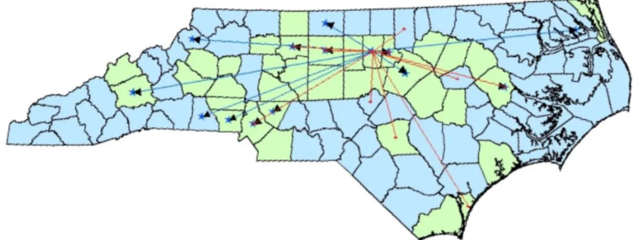
Aggregation from zipcode to county results in 102 location alternatives (i.e., move to any of the 100 coun-ties, move out of NC, or become inactive), which presents too many alternatives for a multinomial logit estima-tion that also includes uncondiestima-tional explanatory variables.6 I examined county-to-county moves to determine whether consideration of adjacent counties only might be a reasonable way to narrow the choice set. To demon-strate the complexity of county-to-county movement, Figure 2.1 shows the origination and destination counties for physicians who moved from 2003 to 2004, with the end destination for each move indicated by a black arrow and the blue dot is the centroid of the county.
To make clear the variety of destinations, Figure 2.2 focuses on movement of physicians from one county (Orange County) in one year (2003-2004). Orange County is one of the most populated counties in NC and contains a large, public research and teaching hospital. In one year, there were 27 physicians who moved from Orange County (denoted by blue lines) and 13 physicians who moved to Orange County from other counties (denoted by red lines). Although physicians may move to neighboring counties, the majority of moves were across the state to non-neighboring counties. Physician movement out of urban Orange County also included both rural and urban destinations (where urban counties are denoted in green and rural counties are denoted in
6
Figure 2.1: Physician Movement within NC, 2003-2004
blue). Table 2.1 shows the average distance (in miles) of moves within NC using centroid to centroid calculation at the county level, where the average distance for all physicians who moved is around 61 miles.
Table 2.1: Summary Statistics: Average Distance of Moves in Miles
Year Mean Std Min Max Median Freq
2004 87.48 63.33 13.72 433.36 74.97 367
2005 63.09 59.35 8.93 378.74 38.09 1241
2006 62.86 60.50 8.93 434.60 37.03 1117
2007 60.84 53.50 12.17 407.36 38.68 729
2008 61.59 57.15 12.17 413.89 38.38 818
2009 59.68 54.77 11.26 373.75 37.31 1062
2010 53.57 50.03 11.26 341.64 33.50 863
2011 61.34 56.58 11.26 384.85 38.68 916
2012 52.56 50.06 8.93 376.61 32.22 1076
Total 60.78 56.38 8.93 434.60 38.09 8189
Note: Statistics are based on 8,189 physicians who moved to a different county within NC in any given year.
To further explore movement, I summarize physician location within NC by urbanicity/rurality of the county and of the zipcode within the county in Table 2.2.7 Around73.3percent of physicians employed in an urban county are in an urban zipcode, while around14.2percent of physicians in a rural county are in a rural zipcode.
Table 2.2: Location by Urbanicity/Rurality of County and Zipcode
Urban Zipcode (%) Rural Zipcode (%) Marginals (%)
Urban County (%) 73.26 6.43 79.69
Rural County (%) 6.14 14.17 20.31
Marginals 79.40 20.60 100.00
Note: Statistics are based on 165,668 person-year observations among active physicians including
their first year in the sample.
Conditional on being active in NC in a given year, a physician may remain in the same location of employ-ment in NC, move within NC, move out of NC or become inactive in the next year. Table 2.3 shows the activity and location outcomes by year. Over 83 percent of year-to-year observations involve no change in activity or location, 12 percent involve a move within NC and 2.5 percent involve a move out of state, while less than two percent of transitions are to inactivity. A majority of the physicians who changed zipcode of employment moved
7
within the county instead of out of the county. Among active physicians in NC, 12 percent change zipcode of employment. Of physicians who moved, 60 percent moved within their counties, while 26 percent moved out of the county to an urban zipcode and 14 percent moved out of the county to a rural zipcode. In light of the computational and data constraints discussed above and in an effort to preserve the urban/rural distinction that characterizes zipcodes and counties, I differentiate location alternatives in the empirical model by moves within and across counties and by urbanicity/rurality of the destination zipcode as summarized in Table 2.3.
Table 2.3: Summary Statistics: Activity and Movement by Year
Activity and Movement Year
Remain in the Same Location in NC
Move within
NC Move out of NC
Become Inactive
2003 91.75 3.98 1.84 2.43
2004 76.41 17.96 4.26 1.37
2005 80.37 14.12 3.15 2.36
2006 86.92 9.17 2.22 1.7
2007 86.41 9.46 2.31 1.82
2008 83.14 12.07 2.76 2.02
2009 82.05 15.25 1.44 1.26
2010 82.92 13.44 2.4 1.24
2011 81.45 14.72 2.23 1.6
Total 83.42 12.36 2.48 1.73
Movement and Rurality Conditional on a Move within NC
Year
Move within the County to an Urban Zipcode
Move within the County to a Rural Zipcode
Move out of the County to an Urban Zipcode
Move out of the County to a Rural Zipcode
2003 34.49 7.72 38.74 19.06
2004 49.32 8.38 27.03 15.27
2005 45.75 8.2 29.93 16.12
2006 47.62 7.88 27.66 16.85
2007 45.59 7.56 30.13 16.72
2008 47.33 6.17 29.6 16.9
2009 65.33 5.87 18.45 10.34
2010 61.15 5.59 23.82 9.44
2011 58.97 5.88 24.6 10.55
Total 53.14 6.87 26.29 13.71
Note: Statistics based on 165,668 person-year observations including a physician’s first year in the survey.
Facility
The physician licensure database also provides current type of facility in the primary, secondary, and ter-tiary locations of employment. The twelve facility types are: locum tenes,8 solo practitioner’s office, free-standing clinic, group office, staff or group model HMO, hospital-outpatient department, hospital-emergency room, hospital-other, medical school or parent university, nursing home/extended care facility, telemedicine, and others. Missing values in facility type are replaced using a similar procedure as with primary location of
8
practice. The previous or future facility type serves as the facility type in a year when it is not reported if zip-codes match across years of primary, secondary, or tertiary location of employment. To simplify the number of categories of facilities, I group the facilities into six categories: group practices, solo practices, hospital-ER re-lated, hospital-Not ER rere-lated, Medical School/Parent University, and others. Table 2.4 displays the distribution of facility type among physicians in NC by year.
Table 2.4: Summary Statistics: Primary Facility Type
Year Group Solo
Hospital: ER
Hospital: Non ER
Medical School
Other
2004 51.45 14.53 5.74 17.62 8.69 1.98
2005 50.40 15.23 5.58 16.99 9.32 2.47
2006 49.13 14.63 5.49 16.99 10.51 3.25
2007 48.58 14.14 5.63 17.65 10.67 3.33
2008 47.67 13.58 5.76 18.56 10.93 3.50
2009 47.93 13.02 5.68 19.30 10.85 3.21
2010 47.25 12.38 5.74 20.11 11.31 3.21
2011 46.17 11.91 5.77 21.34 11.59 3.23
2012 45.49 11.58 5.89 22.13 11.67 3.25
Total 48.06 13.33 5.71 19.13 10.70 3.08
Note: Statistics based on 155,767 person-year observations among active physicians excluding their first year in the sample.
Table 2.5 depicts year-to-year probabilities of changing facility and changing county conditional on staying active in NC. A relatively larger proportion of physicians (20.38 percent) change facility when they change locations than physicians who change facility but not location (7.07percent).
Table 2.5: Location and Facility Change Summary Do Not Change
Facility
Change Facility Total
Remain in the Same Location in NC 92.93 7.07 100 Move within the County to an Urban Zipcode 84.03 15.97 100 Move within the County to a Rural Zipcode 83.36 16.64 100 Move out of the County to an Urban Zipcode 73.13 26.87 100 Move out of the County to a Rural Zipcode 73.07 26.93 100
Total 79.62 20.38 100
Note: Statistics based on 158,682 represents the person-year observations among active physicians excluding their first year in
Hours of Direct Patient Care
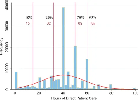
Each active physician provides average hours worked per week in the locations of practice. In estimation, I focus on the number of self-reported direct patient care hours (i.e., I do not model non-patient-related activities). I cap the number of patient care hours at 100 hours per week, which is over two standard deviations above the mean. In the research sample, there are only 914 person-year outliers who reported greater than 100 hours per week and 8,106 (5.2percent) report zero hours of direct patient care. African Americans report a greater average number of hours of direct care than any other group while Caucasians report the lowest average number of hours. Female physicians report fewer patient care hours on average than their male counterparts across all races. Figure 2.3 depicts a histogram of hours of direct patient care using all person-year observations of active physicians (with specific percentiles in red).
Figure 2.3: Histogram of Hours of Direct Patient Care
10% 25% 75% 90%
32 50 60
0
10000
20000
30000
40000
Frequency
0 20 40 60 80 100
Hours of Direct Patient Care
15
2.3.2 Specialty, Experience, and Demographics
Specialty
Although physicians are allowed to update their primary/secondary areas of practice specialty each year, less than 1 percent of physicians in the research sample change their primary area of practice. There are 166 specialties recorded in 2003 and 55 additional specialties appear in the ten subsequent years of observable data. In total, there are 221 different types of medical specialties listed in the database.
Rather than model selection among 221 alternatives, I collapse the large number of physician specialties into five categories that conform to the guidelines set forth by the AMA: (1) primary care physicians/generalists, (2) medical specialists, (3) surgical specialists, (4) hospital-based specialists, and (5) other specialists. Primary care physicians, or generalists, act as the first contact and principal care provider for patients. They also coordi-nate between patient and specialist if additional care is needed. Unlike specialists, generalists require minimal diagnostic and therapeutic technology. Unlike generalists, specialists are trained to handle illnesses that may not occur frequently and that are more serious in nature. They are also more dependent on capital, such as equipment, laboratories, and advanced diagnostic technologies. Therefore, specialists are more likely to be con-strained by their surrounding resources than generalists and are more likely to be attracted to environments with higher concentrations of technological capital. Also, specialists are differentiated by the degree of interaction with patients.
Areas of expertise that fall under generalist include family medicine, general internal medicine, general pediatrics and general OB/GYN. Medical specialists include those in allergy and immunology, cardiovascular disease, dermatology, gastroenterology, internal medicine sub-specialties (such as diabetes, endocrinology, geri-atrics, hematology, infectious disease, nephrology, nutrition, and medical oncology rheumatology), pediatric subspecialties, pediatric cardiology, and pulmonary disease. Surgical specialists are those in general surgery, colon/rectal surgery, neurological surgery, obstetrics and gynecology, ophthalmology, orthopedic surgery, plas-tic surgery, thoracic surgery, and urology. Hospital-based specialists in are anesthesiology, anatomic/clinical pathology, and radiology. Other specialists have expertise in occupational or preventative medicine, or in mental health fields, such as rehabilitation and psychiatry.
Table 2.6: Summary Statistics: Distribution of Specialty by Race and Gender
Primary-Care /Generalist
Medical Specialist
Surgical Specialist
Hospital Specialist
Other Specialist
Race
Caucasian 35.03 16.28 21.32 20.69 6.69
African American 51.48 10.54 17.83 13.79 6.37
Asian 45.22 16.73 13.58 17.06 7.41
Hispanic 44.43 10.73 17.12 19.02 8.70
Other 44.02 16.13 15.32 18.08 6.44
Total 38.13 15.72 19.79 19.58 6.77
Gender
Male 32.78 17.15 22.58 21.00 6.20
Female 50.75 12.36 13.24 15.54 8.11
Total 38.13 15.72 19.79 19.58 6.77
Note: Statistics based on 29,908 uniquely-identified physicians in the research sample. The percentage reported is the row percentage by
race and gender.
Experience
Table 2.7: Summary Statistics: Experience by Race and Gender
Median Mean
Race All Male Female All Male Female
Caucasian 7 9 3 10.73 12.38 6.18
African American 1 2 1 5.64 6.72 4.38
Asian 1 1 1 4.53 5.10 3.56
Hispanic 1 1 1 4.66 5.22 3.68
Other 1 1 1 4.19 4.78 3.02
Figure 2.4: Race Distribution of US Physicians by Graduation Year, 1980-2012
0 0.1 0.2 0.3 0.4 0.5 0.6 0.7 0.8 0.9 1
P
E
R
C
E
NT
A
GE
Black Hispanic Amr Indian Asian White
Demographics
26.5percent are minorities. Compared to the census data, there are larger proportions of Caucasian and Asian physicians than the populations of both races in NC. There are fewer African American and Hispanic physicians in NC relative to their population in NC. The gender and racial distributions of physicians change during the ten years of data as more minority and female physicians enter the labor force. Table 2.9 summarizes age of the research sample. On average, male Caucasian physicians in the sample are older with a median age around 50. Female and minority physicians are generally younger.
Table 2.8: Summary Statistics: Physician Gender and Race
Race Male Female Total
Census Percent
Caucasian/Not Hispanic 76.85 65.47 73.46 64.40
African American/Not Hispanic 6.09 12.27 7.93 22.00
Asian 8.96 12.36 9.97 2.60
Hispanic 2.23 3.00 2.46 8.90
Other Race 5.87 6.90 6.18 2.10
Note: Statistics based on uniquely identified 29,908 physicians in the research sample. The last column contains
the demographic information from the 2013 US Census 2013 in North Carolina.
Table 2.9: Summary Statistics: Physician Age By Race and Gender
Median Age Mean Age
Race All Male Female All Male Female
Caucasian/Not Hispanic 43 45 38 44.60 46.46 39.47 African American/Not Hispanic 38 42 35 40.18 42.53 37.43
Asian 37 38 35 39.61 40.97 37.28
Hispanic 38 40 35 40.48 42.17 37.50
Other 37 38 35 39.56 40.67 37.33
2.3.3 Salary Data
Hourly wages reflect the price of an hour of work in a particular labor market. In a high skilled labor market, a worker’s market value is his/her annual salary. In the partial equilibrium analysis of physician labor supply that I perform, I assume that market salary as well as the demand for labor are pre-determined and known to physicians. Unfortunately, the Physician Licensure Database does not contain salary information and, to my
knowledge, there is no publicly- or privately-available salary database for NC physicians at the individual level. To capture variation in physician labor income, I use two datasets: the Physician Salary Survey Report from the Hospital and Healthcare Compensation Service (HHCS) and the NC Occupational Employment Statistics (OES) of Healthcare Practitioners. Salary data from 2003 to 2012 are reported in real dollars with 2003 as the base year.
The HHCS physician survey provides the average salary (Ssf t) for physicians in 48 different specialties (s)
and 6 different facilities (f) across 10 years (t). The survey also reports the 25 percentile (Q1), median, and 75 percentile (Q3) of salaries for each specialty/facility/year combination. The OES database records salaries of health care practitioners in each of the 100 counties in NC for each year. The OES data reflect averages over all health care practitioners, not exclusively physicians. I calculate for each county ka z-score, zkt, to
reflect the number of standard deviations from the average state salary. Using information from both datasets, I am able to construct a physician salary in each of the 100 NC counties for 48 specialties, 6 facilities, and 10 years. Using the interquantile range formula, I solve IQR = Q3sf t −Q1sf t = 2Φ−1(0.75)σsf t ≈ 2720σsf t ≈ 1.349σsf t whereσsf t represents the standard deviation of salaries in each specialty, facility, and year. Using
the formula, average salary for a physician in county k with specialty s in facility f at time t is defined as
Sksf t=Ssf t+ [σsf t×zksf t].9
When county salary data are missing from OES, I infer unknown values through extrapolation using data from the previous years and/or future years and the average wage inflation data collected by the St. Louis Federal Reserve. The wage inflator reflects seasonally-adjusted salaries of private employees, which includes physicians. If multiple years of the data are not known, I extrapolate information from the American Community Survey (ACS) which also reports full-time, year-round employment information for health care professionals in NC at the county level.
In addition to using this constructed average salary variable (which varies by county, year, specialty, and facility), I generate a salary rank variable by year. I arrange salaries of each county in ascending order such that the highest ranking represents the highest salary level in all counties in a particular year. I assign an average salary and the salary rank to each physician in each year based on her county, specialty and facility.
2.3.4 County-Level Data
I obtain county-level data from Log Into North Carolina (LINC), which combines census data from both state and federal agencies. The 100 counties of NC differ greatly in wealth, size, and the demographics of its
9For example, if the average salary of Alamance County physicians is two standard deviations below the mean wage in NC, then all
residents. I link the county-level data with the location of the physician’s primary practice. The county-level data include basic demographic variables that summarize the size, age, and race distributions of the population in each of the 100 counties in NC. Other variables capture characteristics of the county that might describe the local labor market and local amenities that influence movement into or out of a county. These variables include the number of unemployed, income per capita, total retail sales, number of industry establishments, and education-related variables (i.e., public school personnel, public school personnel with a masters level education, average SAT verbal score, average SAT math score, total public school expenditures, and total public school expenditure from the local government). Importantly, the county-level variables also include characteristics of the medical care market in the county. The variables chosen reflect the potential demand for medical care as well as medical care supply-related characteristics (i.e., total number of pregnancies, total number of births, number of hospital beds, number of long-term care beds, and total number of Medicaid eligible and Medicare enrollees). Summary statistics for available county-level data are provided in Table 2.10 and are averaged over the 100 counties by year. The county-level characteristics capture local amenities, the employment market (potentially relevant for both the physicians and spouse), local demand for medical care professionals, and medical care supply characteristics (i.e., complements and substitutes).10
To capture physician supply characteristics more accurately, different types of physicians are aggregated to the county level using the physician licensure database. Detailed physician supply in the county may capture the degree of complementarity or substitutability of different types of physicians. It may also proxy for the local physician network and reflect ease of referral or competition.
Table 2.10: Summary Statistics: County-Level Data of North Carolina
Mean Std. Dev. Min Max
Demographics
Population (10,000s) 9.06 13.15 0.41 96.26
Older Population (65+) (1,000s) 11.11 12.10 0.64 86.11
Caucasian/Non-Hispanic (1000s) 60.82 79.51 2.26 586.20
African American/Non-Hispanic (1000s) 19.48 36.40 0.02 296.22
Asian (1000s) 1.06 4.97 0.01 51.10
Hispanic (1000s) 6.89 13.31 0.10 121.5
Other (1000s) 3.16 8.15 0.05 72.7
Medical Care Market
Births (1000s) 1.24 2.06 0.04 14.90
Pregnancies (100s) 15.11 26.37 0.41 192.33
Hospital Discharges (1000s) 9.83 12.26 0.34 87.82
Acute Care/Hospital Beds (100s) 2.05 3.28 0.00 19.96
Long-term Care/Nursing Home Beds (100s) 4.42 4.99 0.00 31.00
Midlevel Practitioners 62.55 123.39 0.00 922.00
Registered Nurses (1000s) 0.83 1.57 0.01 10.69
Medicaid Eligibles (10,000s) 1.56 1.83 0.08 14.32
Medicare Insured (10,000s) 1.07 1.21 0.06 8.87
Primary Care Physicians 65.35 118.31 0.00 880
Medical Specialists 32.32 80.74 0.00 643
Surgical Specialists 36.35 75.96 0.00 538
Hospital Specialists 33.04 73.08 0.00 547
Other Specialists 12.64 30.94 0.00 228
Amenities
Gross Retail Sales (Billion$) 0.98 2.05 0.01 18.88
Unemployed (100s) 33.45 51.83 1.12 515.15
Per-capita Income (10,000$) 3.00 0.52 1.88 5.17
Industrial Establishments (100s) 21.81 39.25 0.66 285.18
Local Education Expenditures (10 Million$) 2.60 4.67 0.07 33.80
Total Education Expenditures (10 Million$) 10.91 15.78 0.72 114.99
Public School Personnel (100s) 10.10 14.46 0.00 102.40
Public School Personnel with MA (100s) 3.17 5.03 0.12 40.8
Average SAT Math (100s) 4.94 0.33 3.91 5.84
Average SAT Verbal (100s) 4.76 0.33 3.74 5.70
2.4 Theoretical Motivation
This section presents a theoretical model of the professional and geographical decisions of NC physicians. The primary objective of the theory is to motivate the empirical specification in terms of the individual physician and county-level characteristics that affect physician’s professional and geographical decisions. The community characteristics are of particular interest, and I use the theoretical framework to explain how local characteristics enter as both push factors (i.e., increase the probability of leaving an area) and pull factors (i.e., increase the probability of locating in a particular area). The theory also allows me to discuss the assumptions that must be made to reduce the set of location alternatives to a number feasible for estimation. Because the theoretical model is not parameterized, solved, and estimated, I ignore some issues that would complicate full solution of the physician’s optimization problem. I address these concerns after providing the theoretical motivation.
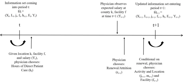
Physicians are forward-looking agents who make decisions based on current utility, budget and time con-straints and discounted expected future utility. Since behavior today affects future utility, I use a dynamic framework in modeling physician’s decisions. I assume that time is discrete with a period being a year. Figure 2.5 displays the timing of physician professional behaviors, where a period is defined as one year. At the be-ginning of periodt, an active physician practicing in NC county or zipcodektand facilityftselects how many
hours (ht) of direct patient care to engage in during this period. At the end of the period, active physicians have
gained an additional year of experience and decide whether or not to renew their NC medical licenses for next period (rt+1). If the physician decides not to renew her license, she attrits from the estimation sample. Con-ditional on renewing the license, a physician decides on activity and location (jt+1) and facility (ft+1) for the next period. Physicians who renew their licenses select whether or not to remain actively practicing medicine. If active, they select the geographical region in which to practice. The alternatives,j, for the activity location decision (jt+1=j) are:
j=
0 inactive
k active in NC in zipcode or countykwherek∈[1, . . . , K] K+ 1 active in NC but not practicing in NC
individual-specific exogenous characteristics (Xt) at timet;11a vector of location characteristics for all counties
in NC (Lt = [L1t, . . . , LKt ], wherek ∈ [1, . . . , K]andK = 850zipcodes or andK = 100counties); and the
history of her previous employment-related behaviors. The pre-determined state variables include specialty (S1) upon completion of medial school and a residency program, current activity and location (jt), current facility
(ft), hours of direct patient care in the previous period, (ht−1), experience up to periodt(Et), and annual salary
for the current period(Yt).12
Figure 2.5: Timing
A physician derives current period utility from both pecuniary and non-pecuniary benefits of working in countykat facilityf at timet. Specifically, the physician receives utility from consumption (Ct), leisure (lt), location characteristics in countyk(Lk
t), the type of facility (ft = f), and an unobserved (by the researcher)
component (εut). At the beginning of each period, the physician selects hours of direct patient care, ht = h,
conditional on the activity, location, and facility selected at the end of the last period. The value of alternative
ht=hat the beginning of periodtis:
Vh(Ωt, εt) =U(Ct, lt, ft=f, Lkt;Xt, Et, ht−1) +εuht
+β{max [W0(Ωt+1), Wj0f0(Ωt+1)j0={1,...K},f0={1,...F}, WK+1(Ωt+1)]} (2.1) ∀t,∀h= 0, . . . ,H
Total consumption is constrained by the annual salary (Yt1[ht >0]) minus the cost of moving (Mt), where
11The vectorX
tincludes variables for age, gender, and birth country/state.
Ct =Yt1[ht >0]−Mt1[jt−1 6= jt]. Leisure (lt) in each period is constrained by total time (Υ) minus hours
worked (ht) and time required to move from one location to another (N), wherelt= Υ−ht−N1[jt−16=jt].
The salary received at timetdepends on physician specialty (St), facility (ft=f), and county (jt=k), where Yt = Y(St, ft, jt). The terminal value of inactive status is denoted by W0(Ωt+1) and the terminal value of activity outside of NC isWK+1(Ωt+1). The value of selecting activity and location (j0) and facility (f0) at the end of the period is:
Wj0f0(Ωt+1) =Et[φj0f0(Lj 0
t , St, ft)×max h0 V
k0f0
h0 (Ωt+1, εt+1)] (2.2)
where φjf reflects the probability of receiving a job offer from facility f0 in locationj0 = k0 and depends on
physician specialty and the contemporaneous location characteristics for each county and facility type.13 The utility a physician receives in the current period depends on the amenities and medical care market characteristics in the previously determined location (jt=k) and facility (ft). To capture effects of habit or a change in routine, I allow current utility to depend on previous hours of direct patient care (ht−1).
At the end of the period, the values of the location and facility for the next period alternatives depend on the current location characteristics (or push factors) as well as the location characteristics of alternative locations (or pull factors). The push factors may influence the location decision directly by lowering the value of staying in the current location via expectation of future levels of those location characteristics. The push factors could also influence the location decision indirectly through hours worked (e.g., high medical demand in a county that leads to long hours in periodtmay raise the value of a new location with lower demand for medical services). The location characteristics may serve as pull factors if they raise the utility of an alternative location. Additionally, characteristics in other locations affect the probability of a job offer.14
2.5 Empirical Framework
Solution to the physician’s optimization problem would yield probabilities of the behaviors (activity, lo-cation, facility, and hours worked) observed in the data. However, the large set of alternatives (among 100 counties or 850 zipcodes and 12 facilities) renders solution and estimation difficult. Although it is possible to
13The model defined in the theoretical section is a partial equilibrium model, where the market demand for physicians is exogenous to
the individual physician and is impacted by exogenous demand-side variables such as county-level demographic, insurance coverage, and other medical care demand characteristics.
14
If we wanted to solve the optimization problem, we must make an assumption regarding a physician’s beliefs about future location characteristics. I could assume perfect foresight or assume that physicians use their current knowledge of all location characteristics (Lt) to forecast the characteristics of each location next period (i.e., Markov beliefs, adaptive expectations). Alternatively, I could
conceptualize the decision problem of physicians as one over all county and facility alternatives within NC, estimation of the probability of moving from a specific county-facility combination to another county-facility is computationally costly if one tries to include observed variables to explain that movement.
To simplify the problem while also retaining as much information about locations as possible, I first collapse location alternatives of active physicians to three: remain in the same zipcode of employment in NC, move to another zipcode of employment in NC, and move outside NC. Conditional on moving to another zipcode of employment in NC, I then expand the location alternatives among those who moved within NC in order to consider four additional categories: move within the county to an urban zipcode, move within the county to a rural zipcode, move out of the county to an urban zipcode, and move out of the county to a rural zipcode. For facility alternatives, I simplify the twelve alternatives to six alternatives. The facility categorization comes from the HHCS physician survey, which was introduced in the data section and is used in my average salary construction. Thus, conditional on remaining active, a physician chooses among six facility types and seven location types. Because it is also important to examine physician labor supply in areas of need, I allow location alternatives to reflect rural and metropolitan counties as defined by the Sheps Center and rurality of zipcode using another method as described further in the Appendix for Chapter 2.
2.5.1 Per-Period Employment Behaviors
Conditional on being active in NC at timet, the redefined activity and location alternatives (jt+1 =j) in the empirical model are:
j =
0 inactive in t+1
1 active in NC and do not change zipcode of employment in t+1
2 active in NC and change zipcode of employment in t+1
3 active and move out of NC in t+1
Conditional on changing zipcode of employment within NC int+ 1, the movement alternativesmt+1=m, are:
m=
1 move within the county to an urban zipcode in t+1
2 move within the county to a rural zipcode in t+1
3 move out of the county to an urban zipcode in t+1
The reduced set of the facility alternatives,ft+1=f, are: f =
1 Group Practice
2 Solo Practice
3 Hospital: ER Related
4 Hospital: Non ER related
5 Medical School/Parent University
6 All other types
I use the theoretical framework to derive demand behaviors as functions of the physician’s information enter-ing periodt,Ωt, and the primitive parameters of the optimization problem (if the utility function parametrization was specified). A first-order Taylor series expansion of the resulting demand functions yields reduced form equa-tions that I specify below. While physicians choose some behaviors (location and facility) jointly, I specify the demand for each behavior but allow for correlation across periods through observed determinants over time (i.e., physician characteristics such as work experience and lagged employment behaviors) and unobserved individual characteristics (such as permanent preferences for living in large cities). The correlation structure also allows for correlation across the many physician behaviors within a time period using observed characteristics as well as time-varying unobserved physician characteristics (such as the birth of a child or an unobserved shock that permeates all employment behaviors within the period). This joint correlation through unobservables is modeled using random effects and requires that I integrate the (conditional) likelihood of the observed outcomes over the distribution of these unobservables, which by definition is unknown. Rather than impose a distributional assump-tion that might be incorrect, I approximate the distribuassump-tion of these unobserved components by estimating the support of the unobserved heterogeneity distribution (using discrete mass points) and their associated weights jointly with the parameters capturing the effects of the observed characteristics (Mroz and Guilkey, 1992; Mroz 1999).15This flexible method allows me to incorporate important omitted (in the literature) aspects of physician employment behaviors such as dependence on past behaviors and simultaneity of many jointly-chosen behaviors. To make explicit the correlation in the resulting probabilities or densities of observed behaviors that form
15
the estimated likelihood function, I decompose the unobserved heterogeneity in each equation into three com-ponents,εet =µe+νte+et, whereµrepresents permanent individual unobserved heterogeneity,νtis
serially-uncorrelated time-varying individual unobserved heterogeneity, andεtis idiosyncratic unobserved
heterogene-ity.16
At beginning of each period, the continuously-valued hours of direct patient care in periodtis a function of the following determinants:17
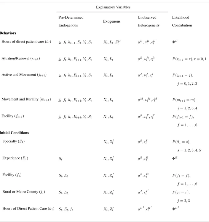
ht=fH(Xt, Et, Yt, Lkt,1[jt= 2],1[mt= 2,4], ft, ht−1, ZtD) +µH +νtH +Ht (2.3)
whereHt is the serially-uncorrelated error explaining variation in hours worked and follows a normal distri-bution andZD are exclusion restrictions that identify (beginning of period) outcomes.18 In addition to its de-pendence on demographic variables, work experience, and salary, the hours outcome depends on current county characteristics, indicators of a recent move and a move to a rural area, current facility type, and lagged hours worked. Empirically, the hours outcome is observed only for those physicians who remain active in NC from the period to the next. This selection is modeled by the following license renewal, activity and location, and facility probabilities.
Conditional on working in countykand facilityf in periodt, I observe the activity, location, and facility outcomes for the next period. However, these outcomes are observed only if a physician is licensed in NC. The probability of not renewing a medical license or attriting from the estimation sample (rt+1= 0) relative to renewing (rt+1 = 1) in periodt+ 1is:
ln(p(rt+1= 0) p(rt+1= 1)
) =fR(Xt, Et+1, Yt, Lkt, ft, ht) +µR+νtR (2.4)
Conditional on not attriting from the sample, the probabilities of being inactive (jt+1 = 0), being active and changing zipcode of employment (jt+1 = 2), or being active and changing employment to outside NC (jt+1 = 3) relative to being active and not changing county of employment (jt+1= 1) in period t+1, are:
16
The subscriptedenotes the relevant behavior: hours (H), activity and location (J, M), and facility (F). Because the unobserved error in each equation is individual specific, the error decomposition, with the individual subscripts i, is:εe
it=µei+νeit+eit. Theoretically,
the permanent component of this specification,µ, is individual specific. Empirically, I estimate this unobserved heterogeneity as a random effect, not as a fixed effect as the notation may suggest. That is, an individuals contribution to the likelihood of her observed behaviors is the product of the probabilities of each behavior,e, conditional on observed explanatory variables and the value of the permanent unobserved heterogeneity, where I integrate the conditional likelihood contribution over the estimated distribution of the unobserved heterogeneity. Similarly,νitis individual specific, and I model it as a random effect. The likelihood function is provided
in section 2.5.3.
ln(p(jt+1 =j|rt+1 = 1) p(jt+1 = 1|rt+1= 1)
) =fJ(Xt, Et+1, Yt, Lkt,1[jt= 2],1[mt= 2,4], ft, ht) +µJ +νtJ
forj= 0,2,3, (2.5)
Conditional on being active and changing zipcode of employment (jt+1 = 2), the probabilities of moving within the county to a rural zipcode (mt+1 = 2), or moving out of the county to an urban zipcode (mt+1 = 3), or moving out of the county to a rural zipcode (mt+1 = 4) relative to moving within the county to an urban zipcode (mt+1= 1) in period t+1, are:
ln(p(mt+1=m|jt+1 = 2) p(mt+1 = 1|jt+1= 2)
) =fM(Xt, Et+1, Yt, Lkt,1[jt= 2],1[mt= 2,4], ft, ht) +µM +νtM
form= 2,3,4 (2.6)
The probabilities of each facility type (ft∈[2,6]), relative to group practice (ft+1= 1) in periodt+ 1, are:
ln(p(ft+1=f|rt+1= 1) p(ft+1 = 1|rt+1= 1)
) =fF(Xt, Et+1, Yt, Lkt,1[jt= 2],1[mt= 2,4], ft, ht) +µF +νtF (2.7)
The empirical framework includes the characteristics of the county in which the physician is currently em-ployed, Lkt, jt =k, instead of the characteristics of each county (Lt). As stated in the beginning of Section 5, the set of activity and location outcomes are reduced from 852 or 102 alternatives (i.e., 850 zipcodes or 100 NC counties, 1 option for outside of NC, and 1 option for inactivity) to a set of seven alternatives for simplicity. This simplification restricts my ability to include county characteristics from other counties, L−tk, where −k
denotes counties that are not chosen. However, if does allow for movement to locations characterized as rural or urban. Thus, the empirical model includes the relevant theoretical push factors on physician professional and geographical outcomes and restricts the pull factors to rural and urban characterizations.
2.5.2 Initial Conditions
Because I first observe (in the data) physicians in the middle of their career, some endogenous state vari-ables are non-zero and present an initial conditions problem in estimation. Rather than treating these varivari-ables as exogenous, I model them using reduced form, static equations. All of the initial condition equations are jointly-estimated with the employment behavior equations and are modeled as functions of exogenous individ-ual characteristicsXtand appropriate exclusion restrictions,ZtI.
US. Additionally, corresponding market characteristics of these locations at year one affect the probability of (1) specialtyS, (2) experience E1, (3) facilityf1, (4) rural or metropolitan location1[j1 = 2,3], and (5) hours of direct patient carehI0, but should not affect the subsequent per-period physician behaviors conditional on these observed initial conditions.
The probabilities of each specialty type (St ∈ [2, . . . ,5]), relative to primary-care/generalist in the first
period, are:
ln
p(St=s) p(St= 1)
=fS(Xt, ZtI) +µS+St fors= 2,3,4,5; t= 1 (2.8)
The continuously-valued level of experience in the first observable period (Et) is specified as:
Et=fE(Xt, St, ZtI) +µE+Et fore= 0, . . . ,69; t= 1 (2.9)
The probabilities of initially-observed facility type relative to group practice (ft= 1) are:
ln
p(ft=f) p(ft= 1)
=fFI(Xt, St, Et, ZtI) +µFI +tFI forf = 2,3,4,5,6; t= 1 (2.10)
The probability of working in a rural county (jt = 2) relative to working in a metro county in the first period
(jt= 1) is:
ln
p(jt= 2) p(jt= 1)
=fJI(Xt, St, Et, ZtI) +µJ
I
+JtI fort= 1 (2.11)
The hours of direct patient care in the first period is specified as:
ht=fH
I
(X, St, Et, ft, ZtI) +µH
I