Perform Pricing Optimization:
A Comparison with Standard
Generalized Linear Models
by Giorgio Spedicato, Christophe Dutang, and Leonardo Petrini
ABSTRACT
As the level of competition increases, pricing optimization
is gaining a central role in most mature insurance markets,
forcing insurers to optimize their rating and consider customer
behavior; the modeling scene for the latter is one currently
dominated by frameworks based on generalized linear models
(GLMs). In this paper, we explore the applicability of novel
machine learning techniques, such as tree-boosted models, to
optimize the proposed premium on prospective policyholders.
Given their predictive gain over GLMs, we carefully analyze
both the advantages and disadvantages induced by their use.
KEYWORDS
applied to policyholder behavior can be found in Dutang (2012).
From a machine learning perspective, the estima-tion of retenestima-tion and conversion represents a super-vised classification problem, traditionally solved in the actuarial practice with a logistic regression. A key advantage offered by logistic regression is the easy interpretability of fitted parameters combined with a reasonable computational speed. Nevertheless, machine learning techniques such as regression and classification trees, random forests, gradient-boosted machines, and deep learners (Kuhn and Johnson 2013) have recently acquired increasing popularity in many business applications.
The interest of actuarial practitioners in machine learning models has grown in recent years (Frees, Derrig, and Meyers 2014; Frees, Meyers, and Derrig 2016). Dal Pozzolo, Moro, and Bontempi (2011) used various machine learning algorithms to predict claim frequency in the Kaggle Allstate competition. In addition, Guelman (2012) showed the benefits of applying gradient-boosting methodologies instead of classical Poisson GLMs for predicting claim fre-quency. While machine learning techniques appear to outperform classical logistic regression in many applications, two issues hamper their widespread adoption in actuarial science. First, their param-eters are often relatively more difficult to interpret (the “black box” issue). Second, the computational time required can be overwhelming, compared with the time required to fit a GLM. To the authors’ knowledge, a systematic review of machine learning techniques comparing predictive performance gain on logistic regression, interpretability, and compu-tational time to model policyholders’ retention and conversion is still lacking in actuarial literature. It will be presented here.
The rest of the paper is organized as follows: Section 2 provides a brief overview of business considerations. In Section 3, we review predictive models and methodologies for binary classification problems. In Section 4, the presentation of a data set is followed by the estimation and comparison of
1. Introduction
Policyholder retention and conversion has received increasing attention within the actuarial practice in the last two decades. In particular, the widespread diffu-sion of Web aggregators has eased the comparison of different insurers’ quotes for customers. Therefore, it is now popular for an insurance company to model not only the cost of the coverage offered but also the insurance demand. Indeed, the likelihood of a pro-spective customer’s accepting a given quotation and the probability of retaining a current customer are key drivers of maintaining and enhancing the profit-ability of an insurer’s portfolio. Such probabilities depend not only on the classical ratemaking variables used to determine expected loss costs, but also on competitive market variables (e.g., distance between insurer’s quote and best/average market price), cus-tomer behavior, and demographics. Actuarial rate-making, current policyholder retention modeling, and prospective policyholder conversion probabilities modeling all aim at so-called pricing optimization (PO). Specifically, this paper aims to investigate how machine learning methodologies can improve policyholder retention and conversion estimation over classical generalized linear models (GLMs).
the policyholders’ loss propensity and the business environment in which the insurer operates. In fact, in almost every country, policyholders can com-pare quotes being offered by multiple competing insurance carriers, making it crucial for the insurer to maximize the gain associated with current and potential policyholders. As a consequence, PO should not only model the prospective cost associated with the coverage provided but also consider the likeli-hood of preventing a customer from accepting deals coming from the competition. More specifically, a conversion analysis should take into account factors such as the individual customer’s demographics, the monetary variation among proposed premiums, and the relative rank of the premium with respect to what is currently offered on the market. A similar analysis, the retention analysis, can be performed in order to estimate the probability of retaining customers.
In practice, performing PO requires four elements: a risk premium model, in order to obtain the expected burning cost; a competitive market analysis to model the competitors’ premiums, given the characteristics of a policyholder; a customer price elasticity model to predict the volume of new business and renewals, reflecting market competition in business analysis; optimization models to integrate all the aforemen-tioned models and predict the profit volume given a change in prices, and to identify the best price changes for a given financial objective. Santoni and Gomez Alvado (2007) and Marin and Bayley (2010) provide a general overview from an insurance perspective.
A review of recent practitioners’ presentations has drawn a few key points to attention. The personal motor business is one in which such techniques have been applied the most, facilitated by policy port-folio sizes and the large volume of data collected. For instance, Guven and McPhail (2013) and Guven (2013) model retention and conversion in U.S. markets using nonlinear GLMs. Another example of PO based on customer value metrics for direct busi-ness can be found in Bou Nader and Pierron (2014). models previously presented, along with an example
of PO. Finally, Section 5 concludes the paper.
In order to achieve these tasks, a real data set coming from a direct insurer will be used in our study. More precisely, the database used is from two recent months of personal motor vehicle liability coverage quotations. Distinct sets of data will be used for the model fitting, the performance assessment, and the PO steps mentioned above. We underline that the methodologies used to model conversions can be transposed to retention modeling without any difficulty. To allow easy replicability of the analy-sis, open source software has been used, such as the R environment (R Core Team 2017) and H2O data mining software (H2O.ai Team 2017).
2. Business context overview
The Casualty Actuarial Society (CAS) defines PO as “the supplementation of traditional actuarial loss cost models to include quantitative customer demand models for use in determining customer prices. The end result is a set of proposed adjustments to the cost models by customer segment for actuarial risk classes” (CAS Committee on Ratemaking 2014, p. 4).
The PO approach includes considerations of both customer behavior and the market environment, thus departing slightly from traditional loss cost–based ratemaking. Although the methodology is innovative, consumer advocates are raising concerns, and there is some initial scrutiny from regulators. For instance, the National Association of Insurance Commissioners (2015) and Baribeau (2015) question to what extent the explicit inclusion of price elasticity in the pro-cess of setting rates makes insurance prices unfair. PO has been extensively treated by actuarial practi-tioners in numerous forms—see, for example, Duncan and McPhail (2013), Guven and McPhail (2013), and Guven (2013)—and to a lesser extent, by aca-demics within insurance science (Rulliere, Loisel, and Mouminoux 2017).
where the performance needs to be measured by methods different from those suggested by classi-cal statistics. Specificlassi-cally, whereas in classiclassi-cal sta-tistics we define a model in order to better explain a phenomenon, in predictive modeling we look at how well a model can make a prediction on unseen data. Moreover, a predictive model emphasizes the importance of assessing predictive performance on a subsample of data different from the one used to calibrate the model.
Regarding the model building process, Kuhn and Johnson (2013) list the following steps:
1. Data preprocessing: This task consists of clean-ing the data, and possibly transformclean-ing predictors (feature engineering) and selecting those that will be used in the modeling stage (feature selection). 2. Data splitting: The data set is divided into a
train-ing, a validation, and a test set, thereby reducing the “overfitting” that occurs when a model appears to perform extremely well on the same data used for finding the underlying structure (e.g., the train-ing set), while showtrain-ing significantly less perfor-mance on unseen data.
3. Fitting the selected models on the training set: Most families of models need one or more tuning parameters to be set in advance to uniquely define the model; these parameters cannot be derived analytically and their class is also known as hyper parameters. A grid search (or an optimized variant) can be employed to find the optimal combination of parameters with respect to a specific mance metric. For binary classification, perfor-mance metrics include the area under the curve (AUC), the Gini index, the logarithmic loss, and the kappa statistic.
4. Model selection: This step involves assessment of which model among the ones tested performs best on a test set, making the results generalizable to unused data.
3.2. Data preprocessing
Data preprocessing techniques generally include the addition, deletion, and transformation of the data. Duncan and McPhail (2013) present four different
approaches that can be used to perform PO:
1. Individual policy optimization: The final price proposed to the policyholder is recalculated at an individual level.
2. Individual policy optimization reexpressed in rate book form: Individually fitted prices are modeled as target variables within a standard predictive model (e.g., a GLM). A traditional rate book struc-ture is thereby obtained.
3. Direct rate book optimization: Very similar to the above method.
4. Realtime optimization: This method stresses the importance of continuously “refreshing” the con-sumer behavior and loss models with data updated in real time.
Although individual policy optimization provides the best performance as judged by revenue maximi-zation, it is worth noting that regulation or operational constraints could lead one to choose less refined approaches.
The current paper focuses its attention on applying predictive modeling to perform conversion modeling as an alternative to standard GLMs. To illustrate, a conversion model targets the dichotomous variable Convert, which can take two values: Convert (Yes), Reject (No). A logistic regression within the GLM family has been traditionally used to address such analysis (Anderson et al. 2007), and it is currently easily applied by taking advantage of actuarial pricing software, e.g., Emblem, Pretium, Earnix, etc.
3. Predictive modeling
for binary classification
3.1. Modeling steps
dictors may be removed to improve interpretability without loss of predictive performance. Many pre-dictive models already contain intrinsic measures of variables’ predictive importance, so they perform an implicit feature selection. Models without feature selection may be negatively affected by uninformative predictors. To avoid this pitfall, specific methodolo-gies have been built in to perform an initial screening of predictors: “wrapper methods” and “filter methods.” Wrapper methods conduct a search of the predictors to determine which, when entered into the model, produce the best result. Filter methods perform a bivariate assessment of the strength of the relation-ship between each predictor and the target.
Further, degenerate or “near-zero-variance” vari-ables (predictors characterized by few distinct values whose frequencies are severely disproportionate) may create computational issues in some models. Principal component analysis and independent com-ponent analysis transformations can be used to reduce the number of input variables, i.e., by using a smaller set of generated variables that seeks to capture the majority of the information, leading to more par-simonious models. Such approaches also prevent multi collinearity, but at the cost of less interpretable variables.
Finally, some predictors require recoding in order to be handled conveniently. For example, encoding nominal or categorical variables into multiple dummy variables is always a necessary step before fitting any model. Manual binning of continuous variables is a widely used approach to overcome marginal non-linearity between the outcome and any continuous variable. However, Kuhn and Johnson (2013) iden-tify three drawbacks of this approach: loss of perfor-mance (since many predictive models are able to find complex nonlinear relationships between predictors, and binning may reduce this feature), loss of preci-sion, and an increase in the false positive rate.
3.3. Model training, tuning,
and performance assessment
Model training consists of fitting a model through an iterative update of variables and/or parameters. This part of the process is crucial for determining the
success or failure of the entire analysis, since most machine learning techniques are sensitive to the format and scale of the predictors.
First, several modeling techniques require pre-dictors to have a common scale of measure. Center scaling is the most commonly used transformation for achieving this objective, helping improve the stability of numerical calculations at the expense of reduced interpretability. In some cases it can also be useful for removing the skewness of the predictors, achieved by taking advantage of methods such as the Box and Cox transformation (Box and Cox 1964).
Second, a proper analysis of outliers is required in many instances. Outliers are observations that appear exceptionally far from the rest of the data and can impact the final performance of the model by intro-ducing a global bias. Usually, a visual inspection of a variable’s distribution is the first step for dealing with this issue, and once the suspect points have been identified, their values should be questioned with care in order to ensure that they indeed belong to the data-generating process. With the exception of some predictive models that are naturally insensitive to outliers (e.g., tree-based models and support vector machines), in all other instances outliers should be removed. In this regard, special techniques such as the spatial sign transformation (Serneels, De Nolf, and Van Espen 2006) can help.
Third, missing values, or observations with no value for some or all variables, should be treated appropriately. As with outliers, a careful exploration into potential structural reasons for such phenomena may be needed. The intuition is that missing data can be caused by a different process underlying data creation, and the simple removal of these data points may negatively affect overall performance. Never-theless, whenever the proportion of missing values is too large to be ignored, methods such as imputation (e.g., k-nearest neighbor model imputation or regres-sion with auxiliary variables) can be used.
pre-step relies neither on a random pre-step nor on a subjec-tive discrete list of hyperparameters, but instead on a probabilistic model.
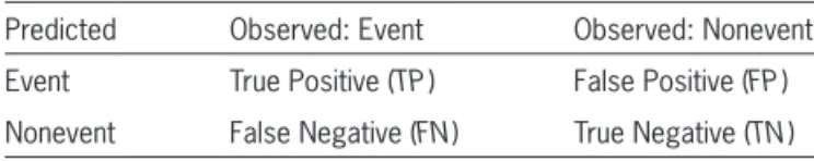
Since our work dedicates most of its efforts to the analysis of a binary response, we offer a special note on how to assess the predictive performance of competing models in such environments. As a pre-liminary step, it is necessary to define a threshold for the probabilities given as predictive outputs by a model in order to determine whether an observa-tion is to be considered an “event” or a “nonevent.” The default threshold is 0.5 (50%), as for a totally random classification. The resulting cross-tabulation of actual and predicted events/non-events after the cutoff has been applied generates a confusion matrix (CM), which becomes the starting point for assessing binary classifier performance.
The structure of a generic CM is given in Table 3.1. Let the total sample size be N = TP + TN + FP + FN. A first measure of classifier precision is the model’s
accuracy Acc: Acc TP TN N
= + . Nevertheless, alter-native measures are generally more appropriate when the outcome distribution is severely unbalanced, as in the conversion-related data set treated in this work.
For example, the kappa statistic, K O E E 1
= −
− , can be
used, where E is the accuracy of the uninformative classifier (the relative frequency of the greatest class), and O is the observed predictive model’s accuracy.
From the CM, two additional statistics for assess-ing binary classification problems can be derived: sensitivity and specificity. Sensitivity is the proba-bility that a sample is correctly classified, given that
it is a true event sample: Se TP TP FN
=
+ . Conversely,
specificity is the probability that a true nonevent is Through this process, the modeler should be
mind-ful of overfitting, which can appear when a model is excessively complex. This is due to a modeling strategy that overemphasizes patterns unique to the specific data set on which the model has been fitted. Overfitted models have poor predictive performance. Thus, it is necessary to obtain a reliable way for esti-mating models’ predictive performance.
Hence, subdividing the data set between a train-ing part, where models are fitted and tuned, and a test part, used to estimate the models’ performance, is fundamental. As further detailed in Kuhn and Johnson (2013), the use of resampling techniques can help one obtain a less biased estimate of model performance. For instance, one approach commonly used is k-fold cross-validation, whereby the training data set is split into k roughly equal-sized subsamples during the estimation process. Once the k models are estimated, the out-of-fold observations are used as a validation set on which the performance metrics fig-ures are computed. Consequently, the overall model fit is obtained by averaging the k cross-validated performance fit estimates.
In addition, when estimating models within a given model family, it must be noted that the vast majority of current machine learning techniques identify models by specifying one or several hyper-parameters. As introduced in the previous section, the optimal values of hyperparameters cannot be directly estimated from data, and hence they require a grid search to tune the final model. The perfor-mance metrics obtained on several models with dif-ferent sets of hyperparameters cannot be (generally) compared with the Cartesian product of all possible combinations. As the computation time or dimen-sionality increases, a random search becomes more appealing. Recently, Bayesian optimization has been gaining popularity as an alternative (Kuhn 2016). Specifically, the Bayesian approach includes a first cycle of random searching to explore the space of the hyperparameters, with a consequent second cycle of numerical optimization based on a Gaussian pro-cess. The advantage of this approach is that every
Table 3.1. CM notation
the midpoint of the probability bucket on the x-axis and the observed empirical event rate on the y-axis. Given a well-performing model, the resulting points would lie on the midline. Lift charts are created by sorting estimated event probabilities in decreasing order. Then the cumulative percentage of samples is plotted on the x-axis, while the cumulative percentage of true events is shown on the y-axis. Lift charts are specifically tailored to compare the discriminating performance of binary classifiers, and they allow one to answer questions such as “What is the expected percentage of total events considering the top per-centage of observations, scored by probability?” Being close to the 45-degree line indicates absence of discriminating advantage, while a perfect classifier would be represented by the hinge function.
Finally, one can decide to apply resampling tech-niques to mitigate instances in which the frequency of binary classes is not even. For example, “down-sampling” reduces the frequency of the most repre-sented class, while “upsampling” randomly draws additional samples from the minority class. Both downsampling and upsampling (and other derived methods) aim to even out the frequency of classes as much as possible.
3.4. Common predictive models
for binary classification
Kuhn and Johnson (2013) organize classification algorithms into three main categories. Linear classi fication models are based on a scoring function that can be expressed as a linear combination of predic-tors. In addition to the classical GLMs introduced by McCullagh and Nelder (1989), the following algo-rithms merit mention:
• Penalized logistic regression (elastic net): The elas-tic net introduces two forms of penalties into the GLM formula, namely the ridge and lasso penalties, which permit better handling of feature selection, overfitting, and multicollinearity (see, e.g., Zou and Hastie 2005).
• Linear discriminant analysis (LDA): LDA finds a linear combination of features characterizing or correctly classified: Sp TN
FP TN
=
+ . The specificity’s
complement to 1 is known as the false classification rate. For a given predictive precision, increasing the sensitivity (i.e., lowering the cutoff probability to identify new samples as events) lowers the specificity.
It is possible to graphically display the trade-off between the two measures by the so-called receiver operating characteristic (ROC) curve, which displays the relation between sensitivity (y-axis) and the false classification rate (x-axis). A model with no discrimi-natory power has an ROC curve along the 45-degree line in the unit square, while a better-performing model exhibits a curve moving toward the top left corner. The ROC curve allows one to obtain a syn-thetic measure of classification power for a given predictive model. The AUC for the ROC curve is a measure bounded between 0.5 (uninformative of the 45-degree line) and 1.0 (perfect discriminatory capability of the Heaviside curve). Finally, the Gini index is a commonly used linear transformation of the AUC: Gini = 2 p AUC − 1.
In practice, the AUC and Gini are certainly the most used metrics to solve binary classification problems. However, while they stress the discrimi-nating power of a predictive model, they are not able to measure how correct the predicted prob-abilities are. Since we want to assess the prediction power, it is also worth exploring different metrics. Therefore our analysis will use the log loss metric,
logloss
N i y p y p
N
i i i i
Σ
(
(
( ) (
) (
)
)
)
= − = + − −
1
log 1 log 1 ,
1
which targets the discrepancy between actual and estimated probabilities, jointly with the AUC and Gini.
• The C5.0 algorithm is one of the most significant representatives of a classical tree-based approach for performing classification (see, e.g., Quinlan 2004). • Random forest blends tree-based logic with the
bootstrap aggregation approach (“bagging”) by creating a so-called forest of trees, rather than a single tree. Each of these trees is a weak learner built on a subset of rows and columns. The classifi-cation from each tree can be seen as a vote, and the most votes determines the classification (see, e.g., Liaw and Wiener 2002). This endeavor successfully reduces variance in the final set of predictions. • A gradient-boosted machine (GBM) applies the
boosting concept on either a regression or a clas-sification tree model. Similarly to bagging, the boosting approach combines the results of multiple models. The key difference is that each subsequent model is recursively applied on the results of the previous one. In particular, as the previous model misclassifies the sample more frequently, more weight starts being given to the subsequent model (see, e.g., Friedman 2001). A notable extension of classical GBM is extreme gradient boosting (XGBoost) (see, e.g., Chen and Guestrin 2016), which has been chosen as the preferred algorithm by winners of many Kaggle competitions.
• Finally, ensembling models of different families often provides higher predictive accuracy than can be obtained by any of the individual models. Such a technique can be based on a super learner, a machine learning algorithm that finds the opti-mal combination of predictions generated by the original constituents (see, e.g., LeDell, Sapp, and van der Laan 2014).
In our numerical experiments, we fitted all of these models. This paper discusses only the most common and best predictive models, a brief outline of which follows.
3.5. GLMs and their elastic net extension
The following section is based on Nykodym et al. (2015), to which the interested reader is directed for details. GLMs extend the standard linear model separating two or more classes of objects or events
(see, e.g., Fisher 1940).
Nonlinear classification models are a heteroge-neous group of techniques, including the following relevant elements:
• Neural networks (and in particular, deep learning, or DL): A DL model consists of multiple strata of “neurons” that collect inputs, transform a linear combination of such inputs into a nonlinear trans-formation through the so-called activation functions, and return the output to the subsequent stratum. DLs have been successfully implemented in a myriad of applications, including image recogni-tion and natural language processing.
• Flexible discriminant analysis (FDA): FDA com-bines ideas from LDA and regression splines. The classification function of FDA is based on a scor-ing function that combines linear hscor-inge functions (see, e.g., Hastie, Buja, and Tibshirani 1995). • k-nearest neighbor (KNN): A KNN model classifies
each new observation according to the most fre-quent class of its k nearest neighbors, according to a specified distance metric. KNN is one of the oldest and most important classifiers found in statistical literature (see, e.g., Fix and Hodges Jr. 1951). • Naive Bayes classifier (NB): NB is based on
the Bayes rule of probability calculus assuming independence among predictors, that is, Pr(Ck|x1,
|x2, . . . ) ∝ pr(Ck)
Π
ni=1Pr(xi|Ck). Despite the strong assumption, predictive performance is often high and computational resources are relatively low (see, e.g., Rish 2001).
• Support vector machines (SVMs): An SVM per-forms classification tasks by creating hyperplanes defined by linear or nonlinear functions (see, e.g., Cortes and Vapnik 1995).
expresses the overall amount of regularization in the model, and its optimal value is usually estimated by a grid search.
Finally, regarding model interpretation, the linear relationship of the explanatory variables underlying a GLM allows one to quickly assess the importance of any terms within the model. The standardized coefficient (the raw coefficient estimate divided by the standard error of estimate) represents a raw mea-sure of the relative importance associated with that variable. The standardized coefficient also serves to determine the p-values of test statistics.
3.6. Random forest
Tree models consist of a series of (possibly nested) if-then statements that partition the data into subsets. The if-then statements define splits that eventually define terminal nodes, also known as “children” or “leaves,” depending on predictors’ values. Given a tree, any new observation has a unique route from the root to a specific terminal node. Trees can be used for either classification or regression problems, and hence they are also known as classification and regression trees (CARTs) (see, e.g., Breiman 2001). Regression trees are used to predict continuous responses, while classification trees are used to predict class proba-bilities. Furthermore, it is possible to convert binary trees into “rules” that are independent sets of if-then statements; this practice can often be advantageous, as pointed out by Kuhn and Johnson (2013). Both tree- and rule-based approaches belong to the family of general partitioning-based classification algorithms.
A number of characteristics explain their popu-larity: (1) They are very interpretable and communi-cable to a non-technical audience; (2) they can handle both numeric and categorical predictors without any preprocessing; and (3) they perform feature selection and can handle missing values explicitly, and any missing value is used as another level/numeric value. However, there are known drawbacks worth mention-ing, such as model instability, possibly leading to big changes in the tree structure given a small change in the data, and suboptimal performance due to their by relaxing the normality and the constant variance
assumptions. The components of a GLM are a random component (from the exponential family and, in our case, the Bernoulli distribution), a systematic com-ponent (that is, a linear combination of explanatory variables and the regression coefficients β, called the linear predictors), and a link function between the mean of the response variable and the linear predic-tors. GLMs are fitted by maximizing log-likelihood, as Anderson et al. (2007) show, using iterative numerical methods. The variable selection task is performed by a chi-square test, as in classical GLMs.
Nevertheless, the extension of GLMs through the elastic net penalty approach has achieved widespread use in machine learning for variable selection and regularization. Here the function to be optimized is max(LogLik − Pen), the penalty1 being l p (α p||β||
1+
(1 − α) p 1
2||β||2. In particular, l > 0 controls the penalty strength while α represents the relative weight of the ridge and lasso components (Nykodym et al. 2016) within the elastic net penalty. The elastic net regularization reduces the variance in the predictions and makes the model more interpretable. In fact, imposing a penalty on coefficient size leads to a sparse solution (throwing off nonsignificant variables) and shrinks coefficients.
The α parameter controls the penalty weight between the l1 (the lasso, that is, the “least absolute shrinkage and selection operator”) and l2 (the ridge regression) penalties. If the l tuning parameter is sufficiently large, it brings coefficient values toward 0, starting from the less relevant ones. As a conse-quence, the lasso has proven to be a good selection tool in many empirical applications. The l2 term is the ridge penalty component, which controls the coefficients’ sum of squares. It is easier and faster to compute than the lasso, but instead of leading to null coefficients, it yields shrunken values. Its advan-tage is that it increases numerical stability and has a grouping effect on correlated predictors. The l value
1||β|| 1=∑
p
k=1|βk| and ||β||2= k1 2
able predictors in order to achieve independence among trees; this parameter controls for overfitting. Suggested values for this parameter are the square root of predictors for classification problems and one-third of predictors for regression problems. 2. Number of independent trees to fit (ntrees):
Increasing this value builds more trees, making the set of predictions more accurate but yielding diminishing returns and requiring more training time. A suggested starting value for this parameter is 1,000.
3. Minimum rows (min_rows): This represents the minimum number of rows to assign to terminal nodes, and it can help against overfitting. The default value for this parameter is 10.
4. Maximum depth of a tree (max_depth): This speci-fies the complexity of interactions for each tree. Increasing the value of this parameter will make the model pick up higher-order interactions and hence can lead to overfitting. A reasonable range for this parameter is [4,14], and the default value is 6. 5. Histogram type (histogram_type): This parameter
determines which type of histogram should be used for finding the optimal split of points in the trees. 6. Row subsample rate (sample_rate): The ratio of
rows that should be randomly collected by the algorithm at every step. A lower value makes the algorithm faster and less prone to overfitting. A reasonable range for this parameter is (0,1], and the default value is 0.632.
Although ensemble methods return a better- performing algorithm overall, they are often con-sidered less interpretable than those of a standard CART. In order to deal with this issue, it is possible to estimate the relative importance of each variable in the regression/classification process.
3.7. The boosting approach:
GBM and XGBoost
A GBM is an ensemble (combination) of regression or classification trees. Unlike random forest models, in which all trees are built independently from one naturally defined rectangular regions. Further,
stan-dard trees are prone to overfitting, since they may find splits in the data that are peculiar to the specific sample being analyzed. Tree pruning techniques have been developed to overcome this specific drawback.
In order to overcome the remaining deficiencies and increase model performance, the endeavor of combining many trees into one model (model ensem-bling) has become the best practice. Specifically, two main algorithms can be used: “bootstrap aggre-gation” (bagging) and “boosting.” Broadly speaking, the bagging approach refers to fitting different trees on bootstrapped data samples, while boosting consists of sequentially fitting trees and giving more weight to the observations misclassified at the previous step. In this paper, both standard and advanced tree-based models will be employed. The C5.0 model (Kuhn et al. 2015) is probably the most prominent example of a standard CART model, but another relevant method known in the literature is the conditional infer-ence tree (Zeileis, Hothorn, and Hornik 2008).
The random forest model (Breiman 2001) takes advantage of the bagging methodology and can be used for both classification and regression problems. Further, it is computationally attractive, since a high number of independent decision trees on different bootstrapped data samples can be built at the same time during the training phase, and the final predic-tions are obtained by averaging the individual scores of each tree. The trees are ideal for bagging, since they can capture the complex structures of interaction in the data, and if developed in sufficient depth, they have a relatively low distortion and, as the trees are notoriously noisy, benefit greatly from averaging.
Our analysis made use of the H2O implementation of the random forest, which introduces some method-ological additions to the original algorithm, as well as a computational optimization achieved by parallelized calculation. Specifically, the main tuning parameters used in this paper for the random forest algorithm are the following:
avail-learning rate, more trees are required to reach the same overall error rate (nround and learning rate are inversely related). A reasonable range for this parameter is [0.10,0.01], and the default value is 0.03.
3. Maximum depth of a tree (max_depth): Same as random forest
4. Minimum child weight (min_child_weight): The minimum sum of instance weight (Hessian) needed to create a final leaf (child). A larger value corresponds to a more conservative model, and it hence helps against overfitting. A reasonable range for this parameter is [1,20], and the default value is 1.
5. Row/column subsample ratio (subsample/ colsample_bytree): The ratio of rows/columns that should be randomly collected/selected by the algorithm at every step. A lower value makes the algorithm faster and less prone to overfitting. A reasonable range for this parameter is [0,1], and the default value is 0.5.
6. Gamma (gamma): The minimum loss reduction for creating a further partition in a given tree. This is a very important parameter that can ease prob-lems related to overfitting. A reasonable range is [0,1], and the default value is 0.
7. Alpha (alpha): The L1 regularization term for weights. It can be used to make a model less aggressive, similarly to gamma. A reasonable range is [0,1], and the default value is 0.
8. Maximum delta step (max_delta_step): In a binary class setting with unbalanced classes (as in our study), it is important to include a constraint in the weight estimation, in order to control every update in a more conservative way. In such instances, a reasonable range is [1,10when enabled]. A value of 0, the default value, means that no constraint is set. i
For simplicity, since the XGBoost parameters out-lined above are very similar to those included in the H2O GBM routine (see, for detail, Jain 2016), we will not relist them in detail for the GBM implementation. another, a GBM sets up a sequential learning
proce-dure, in which every new tree tries to correct the errors of previously built trees, to improve accuracy.
This endeavor, formally known as boosting, sequen-tially combines weak learners (usually CARTs) into a strong learner using an additive approach, yˆi(t) =
Σ
tk=1fk(xi) = yˆ(t–1)i + ft(xi), where each ft(xi) is a tree-based prediction. The peculiarity of the boosting approach is that at every step, the objective function to be optimized aims to reduce the discrepancy between the outcome and the prediction at the previous step, obj(t)=
Σ
ni=1l(yi, yˆi(t)) +
Σ
it=1W( fi) =Σ
ni=1l(yi, yˆ(t–1)i + ft(xi))+W( ft) + constant, a regularization function. The loss function can be any generic loss function and does not have to be only the classical mean square error. The above formula gives more weight to samples badly predicted at previous steps. A gradient-based numerical optimization is used to obtain the model loss. Furthermore, GBM algorithms can be parallel-ized to deliver computationally attractive methods.
Currently, two main variants of classical tree boosting have been proposed, namely Friedman’s GBM (Friedman 2001) and extreme gradient boost-ing (XGBoost) (Chen and Guestrin 2016). Recently, XGBoost has gained popularity among data scien-tists for its faster and better-performing boosting algorithm. In particular, the function to be optimized allows for regularization, algorithms can be naturally parallelized, and cross-validation can be performed at each step.
A number of hyperparameters that need to be tuned are required for the model to be fully specified. Spe-cifically, XGBoost has four possible types of boosters (in our case, trees), and each one comes with dedi-cated parameters. Since our study is taking advantage of the tree booster, the connected employed hyper-parameters are briefly outlined as follows:
1. The number of trees (nround): The maximum number of trees to be built during the iterative boosting process
3. Regularization parameters (l1, l2): It is possible to apply regularization techniques that resemble the lasso and ridge approaches.
4. Loss function (stopping_metric): This is the chosen loss function to be optimized by the model. 5. Adaptive learning parameters (adaptive rate):
When set to True, the following parameters control the process of weight updating and are useful for avoiding local minima: r controls how the memory of prior weights updates and is usually set between 0.900 and 0.999; e takes into account the learning rate annealing and momen-tum, allowing forward progress, and is usually set between 10–10 and 10–4.
6. Number of iterations (epochs): This is the number of passes over the complete training data set to be iterated.
7. Input dropout rate (input_dropout_ratio): This determines what percentage of the features for each training row are to be omitted from training in order to improve generalization.
8. Hidden layers’ dropout rate (hidden_dropout_ ratios): This is the fraction (default set to 0.5) of the inputs for each hidden layer to be omitted from training in order to improve generalization. 9. Maximum sum of the squared weights into neurons
(max_w2): This parameter is helpful whenever the chosen activation function is not bounded, which can occur with maxout and rectifier.
4. Numerical evidence
In this section, we present the data set used for the numerical illustration. Then, we fit a standard GLM to model policy conversion, which will serve as a benchmark against the competing machine learning algorithms. Second, we apply nonlinear and tree-based machine learning techniques to predict policy conversion, and we compare all the methods by accuracy and discriminating power. Finally, we per-form a PO in order to assess the benefits of machine learning techniques compared with the standard approach.
If desired, readers can refer to the H2O booklet for more details (Nykodym et al. 2016). Finally, a grid search approach is necessary to obtain the best con-figuration of the parameters (Peck 2016).
3.8. Deep learning
Neural networks belong to the class of machine learning algorithms used for both classification and regression problems. Lately, they have been success-fully attracting attention in image recognition and natural language processing for their competitive results (see, e.g., Wiley 2016). Neural networks are generally used for detecting recurring patterns and regularities. Those that are characterized by more than one hidden layer are known as deep neural net-works. We will focus our attention on feed-forward deep neural networks, in which signals go from the input layer to the output layer by flowing through the hidden layers, without any feedback loop.
Such a model has a logical structure based on inter-connected processing units (neurons) structured in one input layer, one or more hidden layers, and an output layer. Outputs (signals) from one layer’s neurons to the subsequent layer’s neurons are linearly weighted and then passed to an activation function that can take several forms. Specifically, α=
Σ
ni=1wi× xi + b is the weighted combination of input signals in a generic neuron that is passed to an activation function f (α), where wi is the weight for the xith observation, while b represents the bias node, which behaves in a way similar to the intercept within a linear regression setting.
Given a network structure, the model is fitted by finding the optimal combination of weights, w, and bias, b, that minimizes a specified loss function, and the resulting performance is extremely sensitive to the hyperparameter configuration. Specifically, the main parameters in the framework to be tuned (described in more detail by Arora et al. 2015) are as follows:
1. Network architecture (hidden): This is the num-ber and size of the hidden layers.
are calculated as the ratio and the difference between the company premium and market pre-mium, respectively.
• Vehicle characteristics: vehicleMake, vehicleModel, vehiclePower, vehicleFuelType, vehicleAge, vehicle PurchaseAge, vehicleKm, and vehicleUsage are brand, model, engine characteristics, age, and usage style variables. In addition, vehicleMakeandModel groups the most frequent combinations of vehicle makes and models.
• Demographics: policyholderTerritory and territory BigCity indicate the policyholder’s region of residence and whether it is a high-density city. Policyholder’s age, gender, marital status, and occupation are recorded in the policyholderAge, policyholderGender, policyholderMaritalStatus, and policyholderOccupation variables, respectively. • Insurance and claim history variables: bonus malus
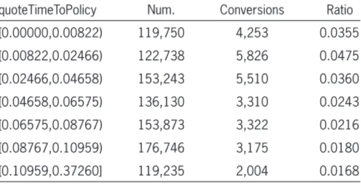
and policyholderPreviousClaims indicate attained bonus-malus level and whether any claims have been filed within the past five years. quoteTimeToPolicy indicates the difference (in years) between the quote and the effective date. Finally, the previousCompany variable indicates whether the previous company was a direct company or a traditional one.
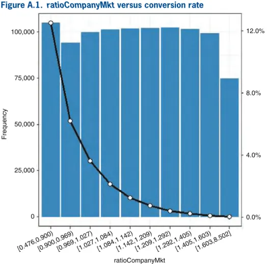
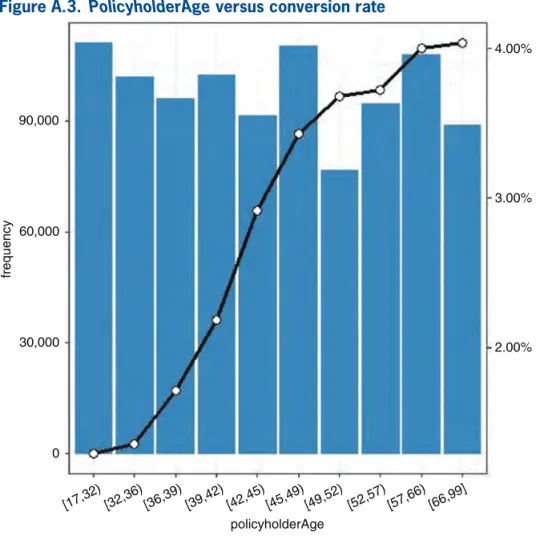
Our analysis focuses on the key variables (the con-version rate and premium variables), as well as other variables. A classical bivariate analysis representing the relationship between conversion rate and selected predictor variables is reported in the appendix.
4.2. Model comparison and selection
The previously fitted models have been used to predict the conversion probability within the test data set. They have been ranked according to perfor-mance metrics, and the best-performing one will be used to predict prospects’ conversion on the test data set and the PO data set. Finally, the obtained results will be compared with those of a GLM model.
Table 4.1 shows the total predicted converted poli-cies in the test data set, along with the log loss and the AUC measure for each model, while the observed total number of converted policies is shown at the top.
4.1. Brief description of the data set
In our study of conversion, we use a database of 1.2 million quotes for fitting and model selection. Furthermore, an additional 100,000 records (the opti-mization data set) are used for the PO exercise. More precisely, we fit the models on the training data set and compare them in terms of predictive performance on the test set. The relevant models have been applied on the PO data set to perform the optimization exer-cise. Table 4.1 shows models’ performance on the training data set, while Table 4.2 shows PO perfor-mance on the optimization data set. Tables display descriptive statistics of the training data set.
The available variables used as predictors are listed below:
• ID and conversion status: quoteId is the database key and converted is a binary variable.
• Premium- and competitive position–related vari-ables: premiumCompany, premiumMarket, and burningCost represent the company’s premium, the market best price (average of the three lowest pre-miums), and the pure premium (loss cost), respec-tively. ratioCompanyMkt and deltaCompanyMkt
Table 4.1. Models’ performance metrics comparison
Model N. of predicted converted Log loss AUC
Observed 6,800 NA NA
XGBoost 6,826 0.0890 0.9064
GBM 6,314 0.0896 0.9050
Random forest 6,817 0.0923 0.8955 Deep learning 7,438 0.0936 0.8925
GLM 6,831 0.0940 0.8896
Note: NA = not applicable.
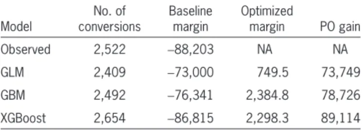
Table 4.2. PO exercise, summary of results
Model conversionsNo. of Baseline margin Optimized margin PO gain Observed 2,522 −88,203 NA NA GLM 2,409 −73,000 749.5 73,749 GBM 2,492 −76,341 2,384.8 78,726 XGBoost 2,654 −86,815 2,298.3 89,114
It is indeed difficult to compare the models in term of computational requirements. Using the H2O package infrastructure, fitting a GLM (even using an elastic net approach) takes a fraction of the time needed to select a model within the cited machine learning approaches. The subjectivity of a hyper-parameter search (grid depth, use of Bayesian opti-mization, etc.), in addition to the time required to fit a hyperparameter-definite machine learning model, explains the difficulty of such comparisons.
The total estimated number of converted policies is calculated as the sum of quote-level estimated conversion probabilities. Clearly, the best model is the one that is able to predict the number of con-verted policies with the highest degree of accuracy, such that the log loss is minimized and the AUC is maximized.
One can observe that all model predictions are quite close to the observed one in terms of num-ber of quotes, with the exception of deep learning. Conversion modeling requires precise assessment of underlying conversion probabilities, which are mea-sured by log loss. By ranking the models according to increasing log loss, it is clear that boosted models (GBM and XGBoost) show the highest performance in terms of predictive accuracy.
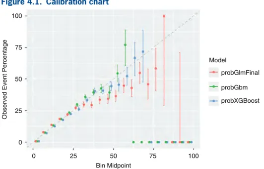
Interestingly, GBM and XGBoost show higher pre-cision in terms of estimated probability when com-pared with a GLM model, even though the underlying conversion probability of most quotes is very low, as the calibration chart (Figure 4.1) shows. Also, they keep estimating the conversion rate unbiasedly at levels of expected outcome higher than in the GLM model. The lift chart (Figure 4.2) shows that there is not much difference between the three predictive models (GLM, GBM, and XGBoost), even if the last two are slightly superior in terms of lift.
0 25 50 75 100
0 25 50 75 100
Observed Event Percentage
Bin Midpoint
Model
probGlmFinal
probGbm
probXGBoost
Figure 4.1. Calibration chart
0 40
20 60 80 100
0 20 40 60 80 100
% Samples Tested
% Samples Found
probGlmFinal probGbm
probXGBoost
The individual PO is carried out as follows:
• The insurer calculates an initial technical premium,
pi0, for the ith prospect, without competitive mar-keting considerations, e.g., adding a fixed loading to the estimated cost, Li.
• On a discretized grid ranging in [p0i (1 −e), pi0(1 +e)], – it computes the conversion probability, pi(pi),
and the expected underwriting result, uwi(pi) (this step also reevaluates the competitive posi-tion for each scenario), and
– it chooses the individual customer’s premium variation to maximize the underwriting result from within the grid.
This approach is known as individual optimization, since it assumes that the insurer is able to target any single prospect with an individual quote. The pres-ence of any marketing and regulatory restrictions would hence lead the insurer to less refined strate-gies, as previously discussed. In addition, this deter-ministic analysis on one period does not take into account any solvency considerations, as well as the renewals of prospects beyond the first period. Also, it assumes no structural changes in the market (e.g., no reactions from competitors) during the process of its implementation.
Thus, it is possible to compare the actual quote number and the observed margin (computed on con-verted quotes) with the amount predicted by each pre-dictive model, as shown in Table 4.2 for the selected elastic net GLM, GBM, and XGBoost models. The final column, “PO gain,” calculated as the differ-ence between the optimized margin and the baseline one, shows the advantage of using an individual PO approach. As previously anticipated, the PO exercise has been carried out on a data set (the optimization data set) that contains quotes used neither to train nor to test the machine learning models.
In Table 4.2, we observe that all boosted models are closer to the observed number of estimated con-versions than is GLM. In particular, the GBM figure is the closest. On the other hand, the estimated margin shows that the XGBoost estimate is very close to the
4.3. Application to PO
The PO process considers knowledge of consumer behavior vital to maximizing expected profit. In our application, the company’s knowledge of consumer behavior is represented by a risk premium model that estimates the expected cost of the insurance cover-age that will be provided, as well as by a conversion model, which estimates the probability of a prospect’s entering the portfolio. Also, information on the com-petitive environment, such as the distance between market price and the company’s premium, should be taken into account.
From a mathematical point of view, we assume that the insurer sets the best premium, p, for each prospect, which maximizes the expected under-writing result, weighted by the conversion prob-ability. That is, uw(p) = p(p) × (p− L), where p(p) is the conversion probability given p, the proposed premium, and L, the expected cost. In the sub-sequent part of the analysis, we will assume that the insurer can modify the proposed premium without any restriction.
The following hypotheses were used to perform the PO exercise:
• The insurer follows an individual optimization approach.
• The individually quoted premium can vary between
−10% and +10% (e) around the baseline.
• The company is able to estimate the expected cost of providing coverage at policy level, Li, thanks to a risk premium model.
• The company calculates the expected underwriting result, uw(pi) =pi− Li.
fraction of the computational time required by most machine learning models. This is because a GLM approach does not require any hyperparameter tuning, unlike the vast majority of machine learning algo-rithms. Precisely since it is not generally possible to find a priori the optimal configuration of the hyper-parameter space, a grid search approach is necessary. The subjectivity of defining the grid space and depth adds another level of complexity when comparing the tuning process and the timing requirements across different families of models.
Acknowledgments
This work has been sponsored by the Casualty Actuarial Society (CAS), the Actuarial Foundation’s research committee, and the Committee on Knowl-edge Extension Research of the Society of Actuaries (SOA). The authors wish to give a special thanks to David Core, director of professional education and research (CAS), and Erika Schulty, research asso-ciate (SOA) for their support.
Finally, the opinions expressed in this paper are solely those of the authors. Their employers neither guarantee the accuracy nor reliability of the contents provided herein nor take a position on them.
Appendix
A.1. Infrastructure
The R software (R Core Team 2017) has been used for this analysis, taking advantage of the packages tidyverse and data.table, as well as the H2O (H2O. ai team 2017) and caret (Wing et al. 2016) machine learning infrastructures.
Parallelization of computing tasks is available for both infrastructures, either on multicore processors or on clusters of computers. Furthermore, the H2O infrastructure permits an easy interface to the Apache Spark framework (Zaharia et al. 2016), specifically devoted to performing parallel processing on big data. Finally, all the software used in the project is open source, making our analysis easily replicable. It is actual figure. It is worth pointing out that the margin
figure should be compared with the total gross pre-mium of around 600,000. After the individual opti-mization exercise has been performed, the “PO gain” column shows that the difference between the base-line and the optimized underwriting margin varies between 74,000 (GLM) and 89,000 (XGBoost).
5. Conclusion
Our work has applied recent predictive modeling methodologies with the goals of taking into account customers’ behavior and of optimizing underwriting margins. The size of the considered data set is rela-tively large compared with the market size, leading to reasonably generalizable results.
We observed that machine learning models may offer higher accuracy and discriminating power when compared with classical GLM models. Our exercise also confirmed the excellent performance of boosted tree-based models. It is still an open question whether the predictive performance gain of machine learning methods is enough to suggest their widespread adop-tion. Interestingly, we found that both the GLM and XGBoost approaches produced very similar results in terms of optimized premium volume. Nevertheless, competitive results of the logistic regression can be explained by the fact that the marginal conversion rate observed for variables that have been found to be extremely important, such as distance between premiums and time to policy, seem monotonic and can be approximately linear (e.g., in the log scale).
Furthermore, we noted that the performance dif-ference between machine learning approaches and classical GLM is relatively higher on the AUC scale than on the log loss scale. This difference can also be visualized by observing the lift curve. Therefore, it is suggested that machine learning models can offer more of a competitive advantage when used for actively marketing to prospective customers, rather than when optimizing the premium amount.
A.3.2. Random forest
H2O Distributed Random Forest can be initial-ized using the code provided in the github reposi-tory. The model was tuned using a random discrete grid search approach and log loss as the criterion. We used two sets of grids: The first one runs over a relatively wide range set of each parameter, the second one on a narrower range. The second grid’s ranges were defined on the basis of the best models found in the previous step.
Precisely, each grid was set to run for both a maximum number of models (200 models) and a maximum amount of time (4 hours). In addition, we judiciously selected the ranges of the tuning param-eters. In the second grid, we used max_depth (8–12), min_rows (10–20), sample_rate (60%–80%), and ntrees (100–300).
A.3.3. Boosting (GBM and XGBoost)
Regarding GBM, we adopted the H2O infrastruc-ture to perform the required preprocessing, as well saved in the following GitHub repository: https://
github.com/spedygiorgio/CasProject2016.
A.2. Tables and figures for
the descriptive section
The overall conversion rate (actual conversions divided by number of quotes) is around 2.5% as shown in Table A.1. Tables from A.2 to A.4 display the con-version rate by each level of key predictors that Fig-ures A.1, A.2, and A.3 graphically depict.
A.3. Models’ specific
implementation notes
A.3.1. GLM
The elastic net approach was used in this analysis, since it allows one to perform variable selection and prevent overfitting and collinearity among predictors, with no dramatic increase in computational time.
Two models were tested:
1. A model with an unbinned coefficient (thus assum-ing marginal linearity of categorical predictors) 2. A model with a binned one. Bins were constructed
on continuous covariates based on deciles.
The log loss criterion identified the unbinned model to be the best-performing one.
Table A.1. Conversion rate summary Converted Num. Freq.
N 103,027 0.9761
Y 2,522 0.0239
Table A.2. Conversion by competitiveness (ratio)
ratioCompanyMkt Num. Conversions Ratio [0.476,0.900) 104,876 13,106 0.1250 [0.900,0.969) 94,077 5,813 0.0618 [0.969,1.027) 99,795 3,624 0.0363 [1.027,1.084) 101,219 2,146 0.0212 [1.084,1.142) 101,721 1,249 0.0123 [1.142,1.209) 102,093 734 0.0072 [1.209,1.292) 102,538 396 0.0039 [1.292,1.405) 101,433 211 0.0021 [1.405,1.603) 99,236 97 0.0010 [1.603,8.502] 74,727 24 0.0003
Table A.3. Conversion by policy effective date delay quoteTimeToPolicy Num. Conversions Ratio [0.00000,0.00822) 119,750 4,253 0.0355 [0.00822,0.02466) 122,738 5,826 0.0475 [0.02466,0.04658) 153,243 5,510 0.0360 [0.04658,0.06575) 136,130 3,310 0.0243 [0.06575,0.08767) 153,873 3,322 0.0216 [0.08767,0.10959) 176,746 3,175 0.0180 [0.10959,0.37260] 119,235 2,004 0.0168
Table A.4. Conversion by policyholder’s age
policyholderAge Num. Conversions Ratio [17,32) 111,121 1,436 0.0129 [32,36) 101,780 1,384 0.0136
[36,39) 96,184 1,652 0.0172
[39,42) 102,495 2,240 0.0219
[42,45) 91,612 2,667 0.0291
[45,49) 110,358 3,780 0.0343
[49,52) 76,675 2,818 0.0368
[52,57) 94,735 3,526 0.0372
[57,66) 107,900 4,314 0.0400
Frequency
[0.476,0.900)[0.900,0.969)[0.969,1.027)[1.027,1.084)[1.084,1.142)[1.142,1.209) [1.292,1.405)[1.209,1.292) [1.405,1.603)[1.603,8.502]
12.0%
8.0%
4.0%
0.0%
ratioCompanyMkt 0
25,000 50,000 75,000 100,000
Figure A.1. ratioCompanyMkt versus conversion rate
Frequency
[0.00000,0.00822)[0.00822,0.02466)[0.02466,0.04658)[0.04658,0.06575)[0.06575,0.08767)[0.08767,0.10959)[0.10959,0.37260]
4.00%
3.00%
2.00%
quoteTimeToPolicy 0
50,000 100,000 150,000
ing of the network (the number and individual size of hidden layers). Some tips can be found in Wpengine (2015). We decided to perform a random discrete search across a hyperparameter space, assuming the following:
1. No more than three hidden layers
2. Size calculated as the number of continuous pre-dictors plus the number of distinct values per each categorical predictor
3. Scoring of the model during training: (1%, 10,000) samples
4. Activation function in each node. All available activation functions were tested (rectified, tanh, maxout, and the corresponding functions “with dropout”).
5. r and e as well as l1 – l2 ranges chosen according to the suggestion of Arora et al. (2015).
We launched a first grid to find a more narrow combination of tuning parameters and defined a as the training and prediction. For hyperparameter
tuning, a grid search was carried out, adopting the random discrete strategy included in H2O, by training up to 100 models for a maximum of 4 hours during the first cycle. Further, we performed a second and finer grid search on the same parameters. In contrast, we used the dedicated library to implement XGBoost models: As a preliminary step, we one-hot encoded cat-egorical variables and simultaneously created a sparse matrix to improve computational efficiency. Next, we performed an initial Cartesian grid search on param-eters of main importance. Then we carried out a more refined tuning grid search on some parameters, and we included max_delta_step to take into account the presence of unbalanced classes. Finally, we optimized the learning rate and the number of rounds jointly.
A.3.4. Deep learning
Generally there are no definite rules for optimal architecture design, in particular regarding the
layer-frequency
[17,32) [32,36) [36,39) [39,42) [42,45) [45,49)[49,52) [52,57)[57,66) [66,99]
4.00%
3.00%
2.00%
policyholderAge 0
30,000 60,000 90,000
Frees, E. W., R. A. Derrig, and G. Meyers, Predictive Modeling
Applications in Actuarial Science, Vol. 1, New York: Cam-bridge University Press, 2014.
Frees, E. W., G. Meyers, and R. A. Derrig, Predictive Modeling
Applications in Actuarial Science: Volume 2, Case Studies in Insurance, International Series on Actuarial Science, New York: Cambridge University Press, 2016 .
Friedman, J. H., “Greedy Function Approximation: A Gra-dient Boosting Machine,” Annals of Statistics, 29:5, 2001, pp. 1189–1232.
Fu, L., and H. Wang, “Estimating Insurance Attrition Using Survival Analysis,” Variance 8:1, 2014, pp. 55–72.
Guelman, L., “Gradient Boosting Trees for Auto Insurance Loss Cost Modeling and Prediction,” Expert Systems with Applica
tions 39:3, 2012, pp. 3659–3667.
Guelman, L., M. Guillen, and A. M. Perez-Marin, “Random Forests for Uplift Modeling: An Insurance Customer Reten-tion Case,” in Modeling and SimulaReten-tion in Engineering,
Economics and Management, Lecture Notes in Business Information Processing no. 115, edited by K. J. Engemann and A. M. Gil-Lafuente, Berlin: Springer, 2012, pp. 123–133, doi:10.1007/978-3-642-30433-0_13.
Guillen, M., and L. Guelman, “A Causal Inference Approach to Measure Price Elasticity in Automobile Insurance,” Expert
Systems with Applications 41:2, 2014, pp. 387–396.
Guven, S., “II-4: Intelligent Use of Competitive Analysis,” paper presented to Ratemaking and Product Management Seminar, March 11–13, 2013, Casualty Actuarial Society.
Guven, S., and M. McPhail, “Beyond the Cost Model: Under-standing Price Elasticity and Its Applications,” Casualty Actuarial Society EForum, Spring 2013, pp. 1–29.
H2O.ai Team, H2O Machine Learning Software, H2O.ai, 2017, http://www.h2o.ai.
Hastie, T., A. Buja, and R. Tibshirani, “Penalized Discriminant Analysis,” The Annals of Statistics 23:1, 1995, pp. 73–102. Hung, S.-Y., D. C. Yen, and H.-Y. Wang, “Applying Data Mining
to Telecom Churn Management,” Expert Systems with Appli
cations 31:3, 2006, pp. 515–524.
Jain, A., “Complete Guide to Parameter Tuning in XGBoost (with Codes in Python),” Analytics Vidhya, March 1, 2016, https://www.analyticsvidhya.com/blog/2016/03/complete-guide-parameter-tuning-xgboost-with-codes-python/. Kuhn, M., “Optimization Methods for Tuning Predictive Models,”
paper presented to Cambridge (UK) R User Group, 2016. Kuhn, M., and K. Johnson, Applied Predictive Modeling,
Amsterdam: Springer, 2013.
Kuhn, M., S. Weston, N. Coulter, and M. Culp, “C50: C5.0 Decision Trees and Rule-Based Models,” Comprehensive R Archive Network, 2015, http://CRAN.R-project.org/ package=C50.
LeDell, E., S. Sapp, and M. van der Laan, “Subsemble: An Ensemble Method for Combining Subset-Specific Algorithm Fits,” Journal of Applied Statistics, 41:6, 2014, pp. 1247–1259. Liaw, A., and M. Wiener, “Classification and Regression by
Random Forest,” R News 2:3, 2002, pp. 18–22.
second one using a more narrow parameter range, defined on the basis of previous results.
References
Anderson, D., S. Feldblum, C. Modlin, D. Schirmacher, E. Schirmacher, and N. Thandic, A Practitioner’s Guide to
Generalized Linear Models, Arlington, VA: Casualty Actuarial Society, 2007.
Arora, A., A. Candel, J. Lanford, E. LeDell, and V. Parmar, Deep
Learning with H2O (3rd ed.), Mountain View, CA: H2O.ai, 2015, http://docs.h2o.ai/h2o/latest-stable/h2o-docs/booklets/ DeepLearningBooklet.pdf.
Baribeau, A. G., “Price Optimization and the Descending Confusion,” Actuarial Review, September/October 2015, pp. 30–33.
Bett, L., Machine Learning with R, Birmingham, UK: Packt Publishing, 2014.
Bou Nader, R., and E. Pierron, “Sustainable Value: When and How to Grow?,” paper presented to 30th International Congress of Actuaries, March 30–April 4, 2014, International Actuarial Association.
Box, G. E. P., and D. R. Cox, “An Analysis of Transformations,”
Journal of the Royal Statistical Society, Series B (Method ological), 26:2, 1964, pp. 211–252.
Breiman, L., “Random Forests,” Machine Learning 45:1, 2001, pp. 5–32.
CAS (Casualty Actuarial Society) Committee on Ratemaking, “Price Optimization Overview,” Casualty Actuarial Society, 2014, http://www.casact.org/area/rate/price-optimization-overview.pdf.
Chen, T., and C. Guestrin, “XGBoost: A Scalable Tree Boosting System,” in KDD ’16: Proceedings of the 22nd ACM SIGKDD
International Conference on Knowledge Discovery and Data Mining, New York: Association for Computing Machinery, 2016.
Cortes, C., and V. Vapnik, “Support-Vector Networks,” Machine
Learning 20:3, 1995, pp. 273–297.
Dal Pozzolo, A., G. Moro, and G. Bontempi, “Comparison of Data Mining Techniques for Insurance Claim Prediction,” Master’s thesis, University of Bologna, 2011.
Duncan, A., and M. McPhail, “Price Optimization for the U.S. Market: Techniques and Implementation Strategies,” paper presented to Ratemaking and Product Management Seminar, March 12, 2013, Casualty Actuarial Society.
Dutang, C., “The Customer, the Insurer and the Market,” Bulletin
Français d’Actuariat 12:24, 2012, pp. 35–85.
Fisher, R. A., “The Precision of Discriminant Functions,” Annals
of Eugenics 10:1, 1940, pp. 422–429.
8th International Conference, June 8–9, 2017, French Asso-ciation of Experimental Economics.
Santoni, A., and F. Gomez Alvado, Sophisticated Price Optimi
zation Methods, Stamford, CT: Towers Perrin, 2007. Serneels, S., E. De Nolf, and P. J. Van Espen, “Spatial Sign
Pre-processing: A Simple Way to Impart Moderate Robustness to Multivariate Estimators,” Journal of Chemical Information
and Modeling 46:3, 2006, pp. 1402–1409.
Wiley, J. F., 2016, R Deep Learning Essentials, Birmingham, UK: Packt Publishing Ltd.
Wing, J., M. Kuhn, S. Weston, A. Williams, C. Keefer, A. Engelhardt, T. Cooper, Z. Mayer, B. Kenkel, the R Core Team, M. Benesty, R. Lescarbeau, A. Ziem, L. Scrucca, Y. Tang, C. Candan, and T. Hunt, “Caret: Classification and Regression Training,” Comprehensive R Archive Network, 2016, http://CRAN.R-project.org/package=caret.
Wpengine, “The Definitive Performance Tuning Guide for H2O Deep Learning,” H2O.ai, February 27, 2015, https://blog.h2o.ai/ 2015/02/deep-learning-performance/.
Yeo, A., K. A. Smith, R. J. Willis, and M. Brooks, “Modeling the Effect of Premium Changes on Motor Insurance Customer Retention Rates Using Neural Networks,” in Computational
Science—ICCS 2001, Lecture Notes in Computer Science no. 2074, edited by V. N. Alexandrov, J. J. Dongarra, B. A. Juliano, R. S. Renner, and C. J. K. Tan, Berlin: Springer, 2001, pp. 390–399, doi:10.1007/3-540-45718-6_43.
Zaharia, M., R. S. Xin, P. Wendell, T. Das, M. Armbrust, A. Dave, X. Meng, J. Rosen, S. Venkataraman, and M. J. Franklin, “Apache Spark: A Unified Engine for Big Data Pro-cessing,” Communications of the ACM 59:11, 2016, pp. 56–65. Zeileis, A., T. Hothorn, and K. Hornik, “Model-Based Recur-sive Partitioning,” Journal of Computational and Graphical
Statistics 17:2, 2008, pp. 492–514.
Zou, H., and T. Hastie, “Regularization and Variable Selection via the Elastic Net,” Journal of the Royal Statistical Society:
Series B (Statistical Methodology) 67:2, 2005, pp. 301–320. Marin, A., and T. Bayley, “Price Optimization for New Business
Profit and Growth,” Emphasis 2010 (1), pp. 18–22.
McCullagh, P., and J. A. Nelder, Generalized Linear Models (2nd ed.), London: Chapman Hall, 1989.
Milhaud, X., S. Loisel, and V. Maume-Deschamps, “Surrender Trigger in Life Insurance: What Main Features Affect the Surrender Behaviors in a Classical Economic Context?,”
Bulletin Français d’Actuariat, 11:22, pp. 5–48, 2011. National Association of Insurance Commissioners, Price Opti
mization, white paper, Washington, DC: National Association of Insurance Commissioners, 2015.
Nykodym, T., T. Kraljevic, N. Hussami, A. Rao, and A. Wang,
Generalized Linear Modeling with H2O (5th ed.), Mountain View, CA: H2O.ai, 2016, https://h2o-release.s3.amazonaws. com/h2o/rel-turing/10/docs-website/h2o-docs/booklets/ GLMBooklet.pdf.
Nykodym, T., A. Rao, A. Wang, T. Kraljevic, J. Lanford, and N. Hussami, Generalized Linear Modeling with H2O (3rd ed.), Mountain View, CA: H2O.ai, 2015, https://h2o-release.s3. amazonaws.com/h2o/rel-slater/9/docs-website/h2o-docs/ booklets/GLM_Vignette.pdf.
Peck, R., “Hyperparameter Optimization in H2O: Grid Search, Random Search and the Future,” H2O.ai, June 16, 2016, https://blog.h2o.ai/2016/06/hyperparameter-optimization-in-h2o-grid-search-random-search-and-the-future/.
Quinlan, R., “Data Mining Tools See5 and C5.0,” RuleQuest Research, 2004, http://www.rulequest.com/see5-info.html. R Core Team, R: A Language and Environment for Statistical
Computing, Vienna, Austria: R Foundation for Statistical Computing, 2017.
Rish, I., 2001, “An Empirical Study of the Naive Bayes Clas-sifier,” Proceedings of IJCAI 2001 Workshop on Empirical
Methods in Artificial Intelligence, 3, pp. 41–46.