Vol 63, No 2 (2020)

(1)

TECHNICAL UNIVERSITY OF CLUJ-NAPOCA

ACTA TECHNICA NAPOCENSIS

Series: Applied Mathematics, Mechanics, and Engineering Vol. 63, Issue II, June, 2020

CONTRIBUTIONS TO THE APPROXIMATION WITH POLYNOMIAL

FUNCTIONS OF MATERIAL SYSTEMS VIBRATIONS.

PART I: THEORETICAL CONSIDERATIONS ON THE

REAL MECHANICAL SYSTEM

Dorin IONIȚA, Mariana ARGHIR

Abstract: The paper presents the approximation of the graphic representations of the measured vibrations for a truck platform, through 10th degree polynomial functions. The approximation by interpolating Lagrange within four distinct measuring points is applied, using the Vandermonde matrix at each analyzed point. Approximation leads to truthful results, so it can be considered valid for the application of vibration analysis of material systems.

Key words: mechanical vibrations, 10th degreepolynomial functions, mathematical approximation.

1. THEORETICAL CONSIDERATIONS

Approximation of vibrations of material systems with polynomial functions of varying degrees is achieved by the classic formula of the Vandermonde matrix [2].

If you want to determine the polynomial coefficients of a "n" degrees polynomial function, of the form:

P_n(x) = a₀ +a₁ x +a₂x₂ + · · · + a_nx_n (1)

If interpolation takes place in "n+1" points, then the coordinate pairs are assumed in the plane:

( , ), ( , ),( , ), … , ( , ) (2)

Each coordinate group of the "n+1" interpolation points will satisfy the relationship (1) and thus will be "n+1" equations, and they will form a system, which can be written in the matrix form, and the form of expression is called the Vandermonde matrix (relation (3)).

⎣ ⎢ ⎢ ⎢

⎡ 1 ⋯ _{1 ⋯}

⋮ ⋮ ⋮ ⋮ ⋮ ⋮

1 ⋯

1 ⋯ ⎦⎥ ⎥ ⎥ ⎤ °

⎣ ⎢ ⎢ ⎢ ⎡

⋮ ⎦⎥

⎥ ⎥ ⎤

= ⎣ ⎢ ⎢ ⎢ ⎡

⋮ ⎦ ⎥ ⎥ ⎥ ⎤

(3)

V a y

In the relation (3) V is the Vandermonde matrix, a is the coefficients column of polynomial function, and y is the non-homogeneity of each polynomial equation. Using the Vandermonde matrix to solve the "n+1" system is particularly difficult and is achieved at high cost. In this situation, the Lagrange interpolation method is applied, which is an alternative way to define the Function Pn(x), without solving the equations system.

1.1. Numerically Approximating Functions

To approximate the functions of one or more variables, numerical analysis uses interpolation polynomials [1].

It is assumed that for n+1distinct argument values x0, x1, ..., xn data in the range [a, b] the

corresponding values of the function:

(2)

The Lagrange interpolation polynomial noted Ln(x), lower degree or equal to n, for

which the points considered the polynomial value corresponds to the value of the function [3]. So:

" ( #) = #, ($ = 0, 1, 2, … , %) (5) The problem is partially solved by the construction of a polynemid, pi(x), in which

&#' () = *#( = +1 !,- . = $,_{0 !,- . / $} (6) Where δij are Kronecker's symbols.

The obtained polynoma cancels those n points x0, x1, ..., xi-1, xi+1, ..., xn and write as

follows:

&#( ) = 0#( 1 )( 1 ) … ( 1 # )

( 1 #2 ) … ( 1 ) (7), and Ci is a constant.

If replaced in relationship (7) x with xi and account is taken of the relationship (6), where pi(xi)=1, it is obtained:

0#( #1 )( #1 ) … ( #1 # )

( #1 #2 ) … ( #1 ) = 1 (8) Of which, it results

0#=₍ 1

#1 )( #1 ) … ( #1 )( #1 ) …( #1 ) (9) With the specified value of coefficient Ci,the

polynomial value pi(x) is calculated, with the expression:

&#( )

=₍( 1 ) … ( 1 # )( 1 #2 )… ( 1 )

#1 ) … ( #1 # )( #1 #2 ) … ( #1 )

(10) With calculated pi(x) polynoma, with the verification of the initial conditions, Lagrange's polynomial is expressed as follows:

" ( ) = ∑ &#4 #( ) # (11) Or

" ( )

= 5 #₍( 1 ) … ( 1 # )( 1 #2 ) … ( 1 )

#1 ) … ( #1 # )( #1 #2 ) … ( #1 ) #4

(12) The relationship (12) contains the expression of polynomial interpolation with the n-degree Lagrange formula.

The uniqueness of Lagrange interpolation polynomial has been demonstrated in the literature. Demonstration is made by RA (Romanian expression, which in English represents DA Discount on Absurd)

2. MECHANICAL SYSTEM

The fundamental study of polynomial approximation through Lagrange polynomials of n - degree, briefly presented in Chapter 1 of this work, can be applied in the analysis of the dynamic behavior of a material system [4].

The mechanical system is the platform of a Mercedes-Benz Actros truck. It is manufactured in 2010, has power 320kW, cylinder capacity 11946 cm3_{, maximum mass 18000kg.}

The truck is equipped with semi-trailer and tarpaulins, as shown in Figure 1.

Fig. 1. Mercedes-Benz Actros 1844 LS truck with

semi-trailer and tarpaulin model 2015 [4]

The mechanical system shown in Figure 1 is a powerful source of vibration, which acts on the human operator, which serves it. The cab of the truck has two seats, occupied by the driver and his help in driving the truck.

3. EXPERIMENTAL MEASUREMENTS

Vibration measurements were performed with the SVAN 958 (Fig. 2), which is a digital analyzer designed for dynamic monitoring, in accordance with ISO 10816, produced by SVANTEK.

(3)

Vibration measurements were performed in eight distinct points on the metal parts of the truck, in sequence:

P1 - gearbox grip screw;

P2 - the support screw of the engine block; P3 - cardan– next to the gearbox;

P4 - trager (intercooler support)- on the heat sink holder;

P5- on chassis next to the engine; P6 – on the screw of the intake gallery; P7 – driver seat;

P8 – in the passenger seat.

The data obtained by measuring vibrations were processed and completed with the SVAN P++ program package and were graphically represented.

3.1. Vibration Measurement

In the figures selected for approximation through Lagrange polynomials there are 4 vibrograms, of which MAX value is considered. The representations were also chosen so that the general theory presented in chapter 1 of the work could be applied.

For each point are given the figure in which is presented the position of the accelerometer on

the motor, it is followed the denomination of the three registered channels in a centralized table. In the table there is only the final mean of the time measurement. The all measurement results are presented in the next figure of the point on the motor.

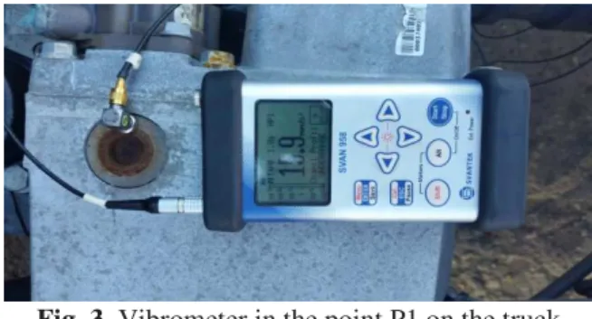
Point P1 - gearbox grip screw

Fig. 3. Vibrometer in the point P1 on the truck

motor

According to Figure3, the measurement axes of the accelerometer present correspondence as follows:

1. Oz axis on measuring channel one – Ch1; 2. Oy axis on the second measuring channel –

Ch2;

3. Ox axis on channel three measurement – Ch3.

Table 1. Measurement results for point P1

Channel Detector Elapsed time

Units Peak P-P Max RMS CRF

Ch1 1 s 00:00:02 mm/s^2 47.86301 89.12509 12.8825 12.67652 3.775722 Ch2 1 s 00:00:02 mm/s^2 47.15199 87.29714 12.8825 12.67652 3.719632 Ch3 1 s 00:00:02 mm/s^2 46.93534 86.69619 12.8825 12.64736 3.711077

Fig. 4. Acceleration graph for point P1

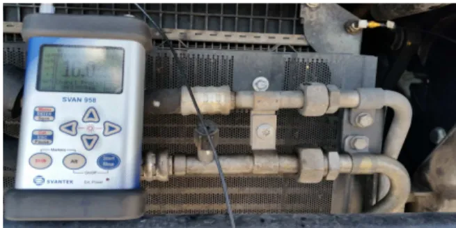
Point P2 - the support screw of the engine block

The vibration measurement mode, at the second point, is illustrated in the figure 5.

Fig. 5. Vibrometer position for the point 2.

Logger results, pixels per sample = 66

14:12:28 14:12:29 14:12:30 14:12:31 14:12:32 14:12:33 14:12:34 Time 14:12:33.500

0.010 0.010

0.011 0.011

0.012 0.012

0.013 0.013

0.014 0.014

m s2

A

c

e

le

ra

ti

o

n

A

c

e

le

ra

ti

o

n

m s2

Start Duration RMS RMS Max

(4)

According to Figure5, the measurement axes of the accelerometer have correspondence with the system axes are coordinated cartesian as follows:

1. Oz axis on measuring channel one – Ch1; 2. Oy axis on the second channel – Ch2; 3. Ox axis on channel three – Ch3.

Table 2. Measurement results for point P2

Channel Detector Elapsed

time Units Peak P-P Max RMS CRF

Fig. 6. Acceleration graph for point P2

Point P4 – pullr (intercooler support) - on the heat sink holder

The vibration measurement mode, using the vibration analyzer, at the fourth point, on the truck pulley considered, is illustrated in Figure no. 7.

Fig. 7. Accelerometer position for the 4 point

According to Figure 7,the measurement channels of the accelerometer present the following correspondence with the Cartesian coordinate axes:

1. Ox axis on measuring channel one – Ch1; 2. Oy axis on the second meas channel – Ch2; 3. Oz axis on channel three meas – Ch3.

Table 3. Results of measurements for point P4

Fig. 8. Accelerations for the P4 point

Point P6 - On the screw at the intake gallery

Vibration measurement mode, using the vibration analyzer, at the sixth point, on the screw at the intake gallery of the truck considered, is illustrated in Figure 9.

According to Figure 9, the measurement channels of the accelerometer present the Logger results, pixels per sample = 66

14:16:32 14:16:33 14:16:34 14:16:35 14:16:36 14:16:37 14:16:38 Time 14:16:35.000

0.010 0.010

0.011 0.011

0.012 0.012

0.013 0.013

0.014 0.014

m s2

A

c

e

le

ra

ti

o

n

A

c

e

le

ra

ti

o

n

m s2

Start Duration RMS RMS Max Info - - Ch1, P1 (HP1, Lin) Ch2, P1 (HP1, Lin) Ch3, P1 (HP1, 1 s) Main cursor 8/22/2015 14:16:35.000 - 0.014 m/s^2 0.014 m/s^2 0.013 m/s^2

Logger results, pixels per sample = 58

14:35:00 14:35:01 14:35:02 14:35:03 14:35:04 14:35:05 14:35:06 14:35:07 Time 14:35:06.500

0.010 0.010

0.011 0.011

0.012 0.012

0.013 0.013

0.014 0.014

0.014 m s2

A

c

e

le

ra

ti

o

n

A

c

e

le

ra

ti

o

n

m s2

(5)

following correspondence with the Cartesian coordinate axes:

1. Ox axis on measuring channel one – Ch1; 2. Oy axis on the second measuring channel –

Ch2;

3. Oz axis on channel three measurement – Ch3.

The time variation law for the registered accelerations is given in the figure 10, for all

the measuremnts. _{Fig. 9. Vibrometer site for vibration measurement} at point P6

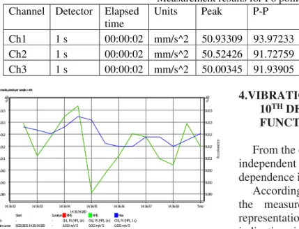
Table 4. Measurement results for P6 point

Fig. 10. Acceleration grapf for the 6 point

Observation.

1. In the experimental study are used only 4 measurement points, that are considered usable for the theory of approximation of graphic functions. 2. The experimental study presented in this

chapter will consider the graphic representations of the points, for the channel that presents the maximum value compared to the other two channels.

1. Each of the four vibrational end points constitutes a different case of study in terms of approximation, so the other two measuring points were not taken into account, in order to be a repetition.

4.VIBRATION APPROXIMATION WITH 10TH_{DEGREES OF POLYNOMIAL}

FUNCTIONS

From the experimental study presented the independent variable is time, and the variable dependence is the acceleration.

According to the measurements performed the measurement step is 10-3_{s, and the} representations were made according to the indications in each table.

It adopts n=10 to solve the problem, and the determination of polynomial coefficients represents the second part of the work, through which a technical problem is solved, through analytical practices.

5. DISCUTIONS. CONCLUSIONS

The theory shown in chapter 1 is universally valid for any material system, whether measurements are made or not different if measurements are followed by graphic representations or not.

This work is tried and proves that the approximation with polynomial functions of the results of the measurements of a real mechanical system is possible and in this way it is established that mathematics is not a sterile Logger results, pixels per sample = 66

14:36:52 14:36:53 14:36:54 14:36:55 14:36:56 14:36:57 14:36:58 Time 14:36:54.500

0.009 0.009

0.010 0.010

0.011 0.011

0.012 0.012

0.013 0.013

m s2

A

c

e

le

ra

ti

o

n

A

c

e

le

ra

ti

o

n

m s2

(6)

science, but it applies to activities in all possible circumstances.

6. REFERENCES

[1] Gheorghe MARINESCU, Analiză numerică, Editura Academiei, R.S. Romania, Bucuresti, 1974ș

[2] Octavian AGRATINI, Ioana CHIOREAN, Gheorghe Coman, Radu TRÂMBIȚAȘ, Analizță numerică și teoria aproximării,

vol. I, Presa Universitară Clujeană, 2002, coordonatori D.D. STANCIU, Gh. COMAN;

[3] Radu TRÂMBIȚAȘ, Numerical Analysis, Presa Universitară Clujeană, 2006;

[4] Andrei Octavian TRITEAN, Contribuții la studiul experimental asupra poluării sonore în transporturi, Raport de cercetare III, Sept. 2014.

Contributii la aproximarea vibratiilor sistemelor materiale cu functii polinomiale. Partea I: Consideratii teoretice asupra unui sistem mecanic real

Rezumat: Lucrarea prezinta aproximarea reprezentarilor grafice ale vibratiilor masurate ale unei platforme de camion, prin functii polinomiale de gardul 10. Se aplica aproximarea prin interpolarea Lagrange in patru puncte distincte de masurare, cu utilizarea matricei Vandermonde in fiecare punct analizat. Aproximarea duce la rezultate veridice, deci poate fi considerata valida pentru aplicarea analizei vibratiilor sistemelor materiale.

Dorin IONIȚA, PhD Student, Technical University of Cluj-Napoca, Department of Mathematics, str. L. Baritiu, nr. 27, Tel: 0745.974.933, E-mail: [email protected] ;

Mariana ARGHIR, Prof. Dr. Technical University of Cluj-Napoca, Department of Mechanical Engineering Systems, B-dul Muncii, No. 103-105, Tel: 0729.108.327; E-mail: