RESEARCH ARTICLE
Machine learning for the prediction
of molecular dipole moments obtained
by density functional theory
Florbela Pereira and João Aires‑de‑Sousa
*Abstract
Machine learning (ML) algorithms were explored for the fast estimation of molecular dipole moments calculated by density functional theory (DFT) by B3LYP/6‑31G(d,p) on the basis of molecular descriptors generated from DFT‑opti‑ mized geometries and partial atomic charges obtained by empirical or ML schemes. A database was used with 10,071 structures, new molecular descriptors were designed and the models were validated with external test sets. Several ML algorithms were screened. Random forest regression models predicted an external test set of 3368 compounds achieving mean absolute error up to 0.44 D. The results represent a significant improvement of the dipole moments calculated using empirical point charges located at the nucleus, even assuming the DFT‑optimized geometry (root mean square error, RMSE, of 0.68 D vs. 1.53 D and R2
= 0.87 vs. 0.66).
Keywords: Density functional theory (DFT), Molecular dipole moment, Quantitative structure property relationships (QSPR), Machine learning (ML), Partial atomic charges
© The Author(s) 2018. This article is distributed under the terms of the Creative Commons Attribution 4.0 International License (http://creat iveco mmons .org/licen ses/by/4.0/), which permits unrestricted use, distribution, and reproduction in any medium, provided you give appropriate credit to the original author(s) and the source, provide a link to the Creative Commons license, and indicate if changes were made. The Creative Commons Public Domain Dedication waiver (http://creat iveco mmons .org/ publi cdoma in/zero/1.0/) applies to the data made available in this article, unless otherwise stated.
Background
The dipole moment (DM) is a widely used parameter, which has been shown to explain observable chemi-cal and physichemi-cal properties of molecules in many differ-ent contexts. Its application in drug discovery, as well as the development of new materials currently attracts high interest [1, 10]. The DM has been useful in the assess-ment of cell permeability and oral bioavailability of drugs, as compounds with large dipole moments are gener-ally more soluble in water and less likely to be absorbed through lipophilic membranes [1, 2]. In two benchmark-ing studies, one with a collection of 467 marketed orally available drugs [1], and the other with 1382 small drugs [2], it was observed that approximately 95% of drugs have DMs lower than 13 D and 10 D, respectively. The same parameter has been used to explain the catalytic activity of enzymes [3], and is commonly included as a descriptor in Quantitative Structure-Activity Relationships (QSAR)
or Quantitative Structure-Property Relationships (QSPR) studies—and often found to be a highly relevant descrip-tor in the best models. A few recent examples are cited here [4–7]. In QSAR modeling of aromatase inhibi-tion [4], antifungal activity [5], and HIV-1 protease/ cyclin-dependent kinases inhibition [7], the molecular DM played a pivotal role as descriptor; it was calculated by molecular mechanics with the SYBYL program [4], or with DFT at the B3LYP/6-31G(d,p) [5] or B3LYP/6-31+G**(6d, 7f) [7] theory levels. An example of a QSPR model employing the DM descriptor is the estimation of micellar properties such as drug loading capacity (LC) [6], for which electronic structure factors and the DM were identified as the most important descriptors; in this case the DM was calculated with the DFT B3LYP func-tional and the 6-311G basis set.
A recent strategy for the design of mechanochromic luminogens was reported based on the DM of donor– acceptor molecules, using a series of 2,7-diaryl-[1,2,4] triazolo[1,5-a]pyrimidine derivatives; the DM was employed to explain and further predict the mecha-nochromic trends, which allowed the authors to design
Open Access
*Correspondence: [email protected]
seven pairs of isomers with opposite mechanochromic trends [8]. Hyperpolarizability and dipole moments are crucial properties of organic non-linear optical mate-rials [9]; although, in general, the hyperpolarizabili-ties depend on the difference between the excited and ground state DMs, in some cases they are proportional to the magnitude of ground sate dipole moments [10].
The application of quantum chemical calculations in organic materials discovery is well established, e.g. to predict electronic properties crucial in the design of organic photovoltaic materials (OPVs), organic-based flow batteries, and organic light-emitting diodes (OLED) [13–15]. Several projects related to drug dis-covery have also employed quantum chemistry calcula-tions; examples include the prediction of protein-ligand interactions and binding energies [11], definition of drug-like chemical spaces [2], and building of large-scale databases of molecular structures and properties [12].
DMs calculated by DFT B3LYP functional hybrid approach revealed an excellent correlation (R2= 0.952)
[2] with experimental values in a data set of 200 small molecules from the CRC Handbook of Chemistry and Physics. Faber et al. [16] reported a mean absolute error of 0.10 D between B3LYP calculations and experiment using 49 molecules. Others have also reported good agreement between experimental and DFT calculated DMs for more complex molecules [17, 18]. Experimental measurements and quantum chemistry calculations were performed in the gas phase.
However, DFT calculations are still computationally too demanding for most large-scale virtual screening explorations, or for the incorporation in fast QSAR or QSPR models. Alternatives have been proposed includ-ing the derivation of DMs from available 3D molecular models and partial atomic charges obtained with empiri-cal or ML methods. Rai and Bakken [19] reported fast and accurate models (random forests) to generate ab ini-tio quality electrostatic potential (ESP) atomic charges, in which atomic descriptors were calculated from the 3D geometries of the molecules, and these charges were used to reproduce the quantum mechanical DMs (aver-age absolute deviation of 1.2 D). Faber et al. [16] reported ML models to predict dipole moments (among other electronic ground-state properties) calculated by DFT at the B3LYP/6-31G(2df,p) level of theory. Screening of sev-eral regressor algorithms combined with various molec-ular representation schemes revealed a best model for DM, based on a graph convolution neural network and molecular graph representation, which achieved a MAE of 0.101 D for a test set of 13,000 molecules. The train-ing set included ca. 118,000 organic molecules with up to nine heavy atoms limited to atomic elements H, C, O,
N, and F [20]. In the same study, random forests yielded MAE between 0.434 D and 0.608 D.
ML from data precalculated by DFT or ab initio meth-ods has emerged as a successful approach to deliver properties of atoms, bonds and molecules with high accuracy at a speed several orders of magnitude higher than would be obtained with the former methods [16, 21]. This requires computationally inexpensive molecular descriptors, available ML algorithms, and well-designed large data sets. ML models are expected to provide early stage filters that can identify promising molecules for further screening, e.g., by computationally more inten-sive methods.
Here we report the exploration of ML tools to predict dipole moments of organic molecules, using a database calculated by B3LYP/6-31G(d,p) for 10,071 structures with atomic elements H, C, N, O, F, S, Cl, Br, P, molecu-lar descriptors based on the DFT-optimized geometries and available schemes for partial atomic charges. The predictions obtained by ML models are also compared with the DM values calculated assuming point charges located at the nucleus of atoms in the DFT geometry, and using partial atomic charges available from empirical and data-driven methods. The DM is a geometry-depend-ent property and the generation/optimization of the 3D structure is exterior to the ML models here described— these were trained to predict the DM for a specific given 3D geometry. DM predictions require a ML model and a 3D structure. If a 3D structure is unavailable, the accu-racy of the predictions will depend on the ML model and on the quality of the 3D structure (obtained by some method independent of the ML model). The possibility of applying the models to external test sets with unknown 3D structures was also assessed by comparing DFT-cal-culated DM values with ML predictions obtained for 3D structures simulated by empirical methods. The “empiri-cal methods” mentioned in this work to generate 3D structures do not use quantum chemistry calculations, but apply rules and molecular mechanics instead.
Methods
Data sets/selection of training and test sets
10,071 molecules with molecular weights (MWs) in the range 40–251 g/mol, and containing up to 19 atoms of elements C, N, O, F, S, Cl, Br, and P. The database was randomly divided into a training set of 6703 molecules, and a test set of 3368 molecules. Two other external data sets (i.e. test set I and test set II) were also compiled from a benchmarking study [2] and an investigation of mech-anochromic materials [8], which comprise 200 small organic molecules with MWs and number of heavy atoms in the range 27–250 g/mol and 2–10, respectively [cal-culated at the B3LYP/6-31G(d,p) level] and a series of 16 derivatives of 2,7-diaryl-[1,2,4]triazolo[1,5-a]pyrimidine [calculated at the B3LYP/6-31G(d) level] containing up to 32 heavy atoms and with a MWs in the range 272–451 g/ mol, respectively.
Geometry optimization and DFT calculations
The calculation of the molecular DM by DFT methods was performed in a semiautomatic way. Starting from SMILES strings or SDF files, the workflow consisted in the genera-tion of the most stable conformer with JChem CXCALC (JChem 15.4.6, 2015, ChemAxon Ltd., Budapest, Hun-gary), optimization of the 3D structure with the GAMESS program [24, 25] using the hybrid B3LYP method [26, 27] and the 6-31G(d,p) basis set, followed by the calculation of the harmonic vibrational frequencies to confirm that the optimized geometry is a minimum on the potential energy surface (all real frequencies) at the same theory level. The molecular DM values were extracted directly from the GAMESS output. Their values range from 0.00 D to 13.18 D, with a mean of 2.91 D and MAD of 1.46 D. The optimized molecular structures and dipole moments were deposited in a public repository [28].
Three-dimensional models of the molecular structures from the test sets I and II were generated with empiri-cal less computationally expensive tools such as CORINA version 2.4 (Molecular Networks GmbH, Erlangen, Ger-many) and Dreiding force field methods (JChem 15.4.6, 2015, ChemAxon, http://www.chema xon.com).
Calculation of molecular descriptors
The dipole moments defined by Eq. (1) were calculated from the DFT-optimized structures and two alternative partial atomic charges—natural bond orbital (NBO) par-tial atomic charges estimated using a ML tool developed in our lab (http://joao.aires desou sa.com/charg es) [29], and Gasteiger partial equalization of orbital electron-egativity (PEOE) partial atomic charges calculated by the ChemAxon CXCALC tool (JChem 15.4.6, 2015, Che-mAxon Ltd., Budapest, Hungary):
where μ is the DM vector, qi is the partial atomic charge
of the atom i, and ri is a vector from the center of mass
to the charge qi. The two resulting values, DMNBO and
DMPEOE, were used as molecular descriptors. Only
mole-cules belonging to the applicability domain of the models to estimate NBO charges [29] were included in the train-ing and test sets. The traintrain-ing and test sets only included molecules belonging to the applicability domain of the models to estimate NBO charges, defined on the basis of the existence of all atom types in the training set of those models; the atom types were specified in terms of the ele-ment and number of H and non-H neighbors [29].
Radial distribution function (RDF) pair descriptors [30] The 3D RDF descriptors were calculated by sampling the function of Eq. (2) at 128 equally distributed values of r between 0 and 12.8 Å:
where N is the number of atoms in the molecule, pi is the
charge of atom i, B is a fuzziness parameter (it was 100 in this study), and rij is the 3D distance between atoms i
and j. Three sets of 128 RDF descriptors were separately calculated, derived from atom pairs with (a) a positive and a negative charge, (b) two positive charges, and (c) two negative charges. Both NBO and PEOE charges were used: RDF_N and RDF_P, respectively.
Projections charges/masses along DM axis (PchmDM) These descriptors were designed to codify the distribu-tion of the charges (and of the masses) projected along the axis of the dipole moment DMNBO or DMPEOE.
PchmDM descriptors were defined as the sum of all charges (or masses) projected onto each of 60 inter-vals of size 0.5 Å on the DM axis between − 15 Å and 15 Å with the origin assigned to the center of mass. Six series of 60 descriptors were generated (360 descrip-tors): (1) desc: sum of all charges at each interval; (2) desc_plus: desc descriptor restricted to positive charges; (3) desc_minus: desc descriptor restricted to negative charges; (4) desc_noH: desc descriptor restricted to non-hydrogen atoms; (5) desc_H: desc descriptor restricted to hydrogen atoms; (6) desc_ mass: sum of all atomic masses at each interval. Both
(1)
�
µ=
n
i=1
qi�ri
(2)
RDF(r)=
N−1
i=1 N
j=1+1
pipje−B(r−rij)
NBO and PEOE charges were used: PchmDM_N and PchmDM_P, respectively.
Geometric CDK descriptors
The geometric descriptors of the Chemistry Develop-ment Kit were calculated with the CDK Descriptor Cal-culator GUI version 1.4.6 (http://www.rguha .net/code/ java/cdkde sc.html): 9 gravitational indices (character-izing the mass distribution of the molecule), 7 moments of inertia (calculates the main moments of inertia, ratios of the main moments and the radius of gyration), and 2 Petitjean shape indices (the topological and geomet-ric shape indices, both measure the anisotropy in a molecule).
Fingerprints
Different types of fingerprints with different sizes were calculated by PaDEL-Descriptor version 2.21 (http:// www.yapcw soft.com/dd/padel descr iptor /) [31] and explored: 166 MACCS (MACCS keys), 881 PubChem fingerprints (ftp://ftp.ncbi.nlm.nih.gov/pubch em/speci ficat ions/pubch em_finge rprin ts.txt), and 1024 CDK (cir-cular fingerprints).
Selection of descriptors
In the quest for QSPR models with the minimum possible number of descriptors, feature selection was performed based on the importance of descriptors assessed by ran-dom forests (mean decrease in accuracy measure) and the CFS (Correlation-based Feature Subset Selection) algorithm [32] implemented in Weka 3.7.12 [33]. In CFS, the heuristic takes into account the usefulness of individ-ual descriptors for predicting the property (DM) together with the level of intercorrelation among them. The exper-iments were conducted with the AttributeSelectedClas-sifier routine of Weka with the CfsSubsetEval option for attribute evaluator and the BestFirst, GreedyStepwise or PSOSearch option as the search method.
ML methods
Random forests (RF) [34, 35]
A random forest is implemented as an ensemble of unpruned regression trees which are created using boot-strap samples of the training set. For each individual tree, the best split at each node is defined using a randomly selected subset of descriptors. Each individual tree is cre-ated using a different training and validation set. A RF yields a final prediction for an object as the average of the predictions of the individual regression trees. The predic-tions obtained for the objects left out of the training are compared to the target values, and deviations are aver-aged in the out-of-bag (OOB) error estimation. In the
experiments presented here, RFs were used for the devel-opment of regression models to estimate DM. RFs were grown with the R program [36], version 3.2.3 using the RandomForest library [37]. The number of trees in the forest was set to 500, the number of descriptors available for each node was optimized and the other parameters were used with default values.
Support vector machines (SVMs) [38]
SVMs map multidimensional data into a hyperspace (a boundary or hyperplane) through a nonlinear trans-formation (kernel function) and a linear regression is then applied in this space. The boundary is defined with examples of the training set—the support vectors. In this study, SVM models were explored with the Weka31 (ver-sion 3.7.12) implementation of the LIBSVM software [39]. The epsilon-SVM-regression type was chosen, the kernel function was the radial basis function with the default gamma parameter, and the parameter C was opti-mized in the range of 10–10,000 through cross-validation with the training set.
Multilayer perceptron (MLP)
The Weka [33] MLPRegressor package (version 3.7.12) was used to implement feed-forward neural networks. It trains a multilayer network with one hidden layer using Weka’s Optimization class by minimizing the squared error plus a quadratic penalty with the BFGS method. The MLPRegressor options were set as default, except the number of hidden units and the ridge parameter that were optimized in cross-validation experiments with the training set.
Gaussian radial basis function (RBF)
A RBF is a feed-forward neural network (NN) with three layers of nodes, the middle (hidden) layer being made up of Gaussian or asymmetric kernels. Only the weights between the hidden layer and the output layer are modi-fied during training. A RBF NN can accomplish a highly nonlinear mapping from the input space onto the out-put space. It was used in this work as specifically imple-mented by the RBFRegressor class in Weka [33] version 3.7.12, with the options set as default, except the number of basis functions and the number of sigma parameters that were optimized in cross-validation experiments with the training set.
Results and discussion
and comparing the results with the DFT DMs—Table 1 and Additional file 1: Figure S1.
There is a clear correlation between the empirical cal-culations and the DFT results, but we expected that these results could be significantly improved with the help of ML. It is noteworthy that although the deviations obtained with DMNBO and DMPEOE are similar, the
inter-correlation between them is relatively low (R2= 0.44) for
the training set, which suggests that both parameters may be complementary and relevant as attributes in a ML approach to predict DFT DMs.
Of course, the application of Eq. (1), which considers charges of atoms located at their nucleus, can only be seen as an approximation to the DM calculated by DFT methods. Furthermore, two additional sources of devia-tions are the uncertainty regarding the 3D geometry and the quality of the charges. In the results of Table 1, the uncertainty from the geometry was avoided, as the DFT-optimized geometry was used, and the partial atomic charges are calculated independent of the geometry. Both PEOE and ML NBO charges were not developed to fit electrostatic potentials or dipole moments, but rather to account for intramolecular effects, e.g. related to reactiv-ity or spectroscopic properties [29]. Therefore, we aimed at ML models that can build on the information con-tained in such charges, by learning from large datasets of DMs calculated with DFT calculations, to improve the ability to predict DMs.
A baseline performance for our models was esti-mated using the Zero Rule algorithm in a ten-fold cross-validation experiment with the training set in Weka, which yielded values for R, RMSE and MAE of − 0.038, 1.841 eV, and 1.447 eV, respectively.
Random forest prediction of molecular DMs
Our ML strategy to predict DMs assumes that the molecular geometry is known from the onset, i.e., the DFT-optimized geometry is used to calculate the 3D molecular descriptors that are presented to the
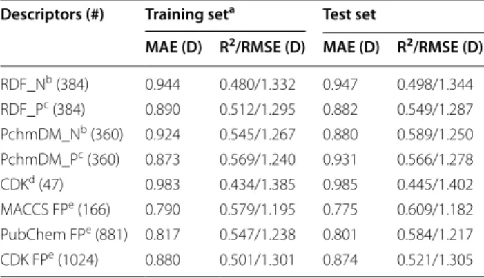
regressors. So, the models are trained to predict the DM for that geometry. The results in Table 1 have shown that this is a task for which common methods are rather limited. Random forests regression mod-els were trained with 6703 molecules represented by the descriptors RDF (with NBO and PEOE charges), PchmDM (with NBO and PEOE charges), geometric CDK descriptors, and other well-established finger-prints such as fragment fingerfinger-prints (166 MACCS keys and 881 PubChem) and circular fingerprints (CDK). The models were validated with the independent test set consisting of 3368 molecules—Table 2. Although the predictive power of the eight models developed (Table 2) was very modest, with RMSE in the range of 1.2–1.4 D for the test set, the best sets of descriptors and fingerprints were selected for further experiments. After the exploration of models derived with 3D molec-ular descriptors and fingerprints, we investigated the inclusion of the descriptors DMNBO and DMPEOE to the
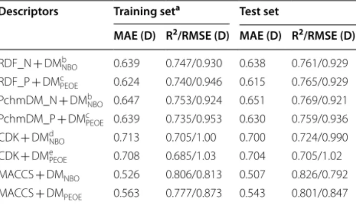
best sets of descriptors and fingerprints—Table 3. The inclusion of both DMNBO and DMPEOE is
advanta-geous, and the best performance was observed with the MACCS fingerprints combined with DMNBO. The good
performance of 2D descriptors (and the observation that the most important 2D descriptors encode for small polar functional groups—see below) indicate that the presence of small polar fragments have a strong impact in the dipole moment of the whole molecule. Descriptors calculated with NBO charges performed slightly better than those with PEOE and were preferentially used in the following experiments. Combinations of 3D descriptors (RDF, PchmDM, CDK), 2D descriptors (MACCS finger-prints), DMNBO and DMPEOE were explored—Tables 4
Table 1 Comparison of DFT DMs with DMNBO and DMPEOE for the 6703 and 3368 chemical structures of the training and test sets, respectively
a The DMs were calculated using the DFT geometry optimization b Training data set
c Test data set
Set Chargea MAE (D) R2/RMSE (D)
Trb NBO 1.44 0.626/1.80
PEOE 0.988 0.650/1.53
Tec NBO 1.44 0.656/1.78
PEOE 0.968 0.659/1.53
Table 2 Prediction of the DFT DM by random forests on the basis of different molecular descriptors
a OOB estimation
b Descriptors calculated using NBO charges c Descriptors calculated using PEOE charges d Geometric CDK descriptors
e Fingerprints
Descriptors (#) Training seta Test set
MAE (D) R2/RMSE (D) MAE (D) R2/RMSE (D)
RDF_Nb (384) 0.944 0.480/1.332 0.947 0.498/1.344
RDF_Pc (384) 0.890 0.512/1.295 0.882 0.549/1.287
PchmDM_Nb (360) 0.924 0.545/1.267 0.880 0.589/1.250
PchmDM_Pc (360) 0.873 0.569/1.240 0.931 0.566/1.278
CDKd (47) 0.983 0.434/1.385 0.985 0.445/1.402
MACCS FPe (166) 0.790 0.579/1.195 0.775 0.609/1.182
PubChem FPe (881) 0.817 0.547/1.238 0.801 0.584/1.217
and 5. The results reveal that the inclusion of CDK descriptors made almost no difference in the results, but increased the calculation time—they were therefore not included in the following experiments.
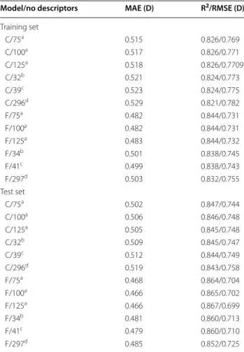
The best models (C and F) yielded MAE of 0.512 D and 0.479 D for the test set, which are approximately 35% and 33% of the MAD from the average (1.47 D). The models are also significantly more accurate than the baseline model described above.
In order to evaluate the robustness of the approach, model C was evaluated using four alternative random
splits of the data set into training and test sets: the test set predictions exhibited R2, RMSE and MAE values in
the intervals 0.82–0.85, 0.75–0.79 D and 0.51–0.53 D, respectively.
The combination of DMNBO and DMPEOE with
dif-ferent type of descriptors achieved the models with the best performance, as can be seen in Tables 4 and 5. However we wanted also to investigate how they perform with each type of descriptors e.g. MACCS FP, RDF (with NBO charges), PchmDM (with NBO charges), geometric CDK descriptors—Table 6.
Simultaneous inclusion of the two DMs (DMNBO and
DMPEOE) to the different types of descriptors studied
allowed to obtain models with a much greater predic-tive capacity than the one obtained without the inclusion of these DMs, for all the experiments the MAE that was obtained is less than or equal to 0.533 D. The best model, standing out in all the prediction parameters of the other models for training and test sets, was achieved using 2D descriptors, MACCS fingerprints. It was impressive for us the performance achieved by this model, yielded MAE of 0.444 D for the test set, using only the MACCS fingerprints and the two DMs calculated (DMNBO and
DMPEOE).
Descriptor selection and optimization of QSPR methods
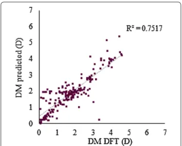
Procedures for feature selection were applied to the descriptors of models C and F—Table 6. The 75 most important descriptors of models C and F were identified by RFs and enabled the training of new RF models with even better prediction accuracies than the models trained with the whole set of descriptors (746 and 912 descrip-tors, respectively). A graphical representation of the pre-dictions versus the DFT-calculated values for approach C and F are shown in Fig. 1. The selected 75 descriptors for approach C included DMNBO and DMPEOE, 58 RDF
descriptors (26 of type a, 15 of type b, and 17 of type c), and 15 PchmDM descriptors (1 of type desc, 1 of type desc_plus, 1 of type desc_minus, 3 of type desc_noH, 3 of type desc_H, and 5 of type desc_mass). Within the top ten descriptors, DMNBO is the most important descriptor,
followed by DMPEOE and RDFs of the three types (six of
type a; one of type b in the 8th position; one of type c in the 5th position). The Pearson correlation coefficients between each of these eight RDF descriptors and the DFT DM are in the range of 0.10–0.45 for the training set.
Similarly, the inspection of the ten most important descriptors of model F revealed DMNBO and DMPEOE as
the first and second most important descriptors, respec-tively. MACCS fingerprints occupy the 3rd, 5th and 10th positions, encoding the presence of nitrile, S = A groups (where A is any atom) and the N atom, respectively. The Table 3 Prediction of the DFT DM by random forests using
DMNBO or DMPEOE
a OOB estimation
b Descriptors calculated using NBO charges, and DM NBO c Descriptors calculated using PEOE charges, and DM
PEOE d Geometric CDK, and DM
NBO e Geometric CDK, and DM
PEOE
Descriptors Training seta Test set
MAE (D) R2/RMSE (D) MAE (D) R2/RMSE (D)
RDF_N + DMb
NBO 0.639 0.747/0.930 0.638 0.761/0.929
RDF_P + DMc
PEOE 0.624 0.740/0.946 0.615 0.765/0.929
PchmDM_N + DMb
NBO 0.647 0.753/0.924 0.651 0.769/0.921
PchmDM_P + DMc
PEOE 0.639 0.735/0.953 0.630 0.759/0.936
CDK + DMd
NBO 0.713 0.705/1.00 0.700 0.724/0.990
CDK + DMe
PEOE 0.708 0.685/1.03 0.704 0.705/1.02
MACCS + DMNBO 0.526 0.806/0.813 0.507 0.826/0.792
MACCS + DMPEOE 0.563 0.777/0.873 0.543 0.801/0.847
Table 4 Prediction of the DFT DM by random forests using NBO charges and combining different descriptors
a OOB estimation
b RDF pairs NBO charges, PchmDM NBO charges, and DM NBO
c RDF pairs NBO charges, PchmDM NBO charges, geometric CDK, and DM NBO d RDF pairs NBO charges, PchmDM NBO charges, DM
PEOE, and DMNBO e RDF pairs NBO charges, PchmDM NBO charges, geometric CDK, DM
PEOE, and
DMNBO
f RDF pairs NBO charges, PchmDM NBO charges, MACCS fingerprints, and
DMNBO
g RDF pairs NBO charges, PchmDM NBO charges, MACCS fingerprints, DM PEOE,
and DMNBO
Models Training seta Test set
MAE (D) R2/RMSE (D) MAE(D) R2/RMSE (D)
Ab 0.627 0.757/0.912 0.623 0.774/0.905
Bc 0.616 0.762/0.903 0.611 0.778/0.896
Cd 0.525 0.823/0.780 0.512 0.846/0.752
De 0.522 0.824/0.777 0.509 0.846/0.750
Ef 0.562 0.790/0.850 0.553 0.807/0.838
remaining positions are occupied by RDF descriptors of type a. The Pearson correlation coefficients between these MACCS descriptors and the DFT DM is in the range of 0.24-0.28 for the training set.
In an additional experiment, the RDF and PchmDM descriptors were discarded from model F, and a new model was re-trained only using MACCS, DMNBO and
DMPEOE descriptors. The results were slightly improved
(training set: MAE = 0.46 D, RMSE = 0.71, R2= 0.85; test
set: MAE = 0.44 D, RMSE = 0.68 D, R2= 0.87) indicating
that the two DMNBO and DMPEOE descriptors together
incorporate the crucial 3D information to deliver the predictive ability of DFT DM here described (Additional file 1: Figure S2).
Further validation was performed using the y -randomi-zation technique. The best C model was rebuilt with 5 modified training sets; the y-column data (DFT DM) was scrambled, keeping the descriptor matrix unchanged. The random models were found to have a considerably lower R2 and higher RMSE compared to those of the
original model (R2 of 0.0005–0.0015 and RMSE of 1.89–
1.91 D for the test set), further corroborating the statisti-cal reliability of the model.
These results compare favorably to those reported by Lilienfeld and co-workers using a kernel ridge regres-sion algorithm trained with 16,000 molecules to predict the DM calculated with the B3LYP/6-31g(2df,p) level of theory, which achieved a MAE of 0.63 D for an external test set [40]. More recently, in the some lab, a ML model developed with a graph convolution neural network and molecular graph representation, obtained a MAE of 0.101 D for a test set of 13,000 molecules [16]. In spite of the large number of molecules that comprise the data set (131,000 molecules), they are limited to five atomic ele-ments (H, C, O, N, and F) and molecules containing up to 9 heavy atoms. The MAD of the DM is 1.17 D for the whole data set [20], which is smaller than for our data set (1.46 D). In order to evaluate the performance of our best C model with molecules made of the same elements, we retrained and re-validated the model without the mole-cules containing S, Br, Cl, or P. The MAD of the data set was reduced to 1.33 D, as was the MAE for the test set of 2667 molecules (0.42 D). The Rai and Bakken ML model to predict B3LYP/6-31G* electrostatic potential partial charges was applied to the calculation of dipole moments using Eq. (1), reporting a MAE of 1.2 D for an external test set of 5000 organic molecules [19]. However, this result is not directly comparable with ours since the DMs were processed as vectors and the deviation was calcu-lated as the size of the difference vector.
Table 5 Prediction of the DFT DM by random forests using a combination of DMNBO and DMPEOE with different type of descriptors
a OOB estimation b Combining DM
PEOE, and DMNBO c RDF pairs NBO charges d PchmDM NBO charges
Models Training seta Test set
MAE (D) R2/RMSE (D) MAE(D) R2/RMSE (D)
MACCSb 0.460 0.853/0.707 0.444 0.872/0.680
RDFb,c 0.533 0.817/0.791 0.522 0.839/0.767
PchmDMb,d 0.540 0.819/0.786 0.533 0.839/0.765
CDKb 0.538 0.815/0.793 0.525 0.837/0.765
Table 6 RF prediction of DM with subsets of descriptors from models C and F
a OOB estimation for the training set
b Using the mean decrease in accuracy measure of importance for the
descriptors in the RF algorithm
c Using the the CFS with BestFirst routine from Weka d Using the the CFS with GreedyStepwise routine from Weka e Using the the CFS with PSOSearch routine from Weka
Model/no descriptors MAE (D) R2/RMSE (D)
Training set
C/75a 0.515 0.826/0.769
C/100a 0.517 0.826/0.771
C/125a 0.518 0.826/0.7709
C/32b 0.521 0.824/0.773
C/39c 0.523 0.824/0.775
C/296d 0.529 0.821/0.782
F/75a 0.482 0.844/0.731
F/100a 0.482 0.844/0.731
F/125a 0.483 0.844/0.732
F/34b 0.501 0.838/0.745
F/41c 0.499 0.838/0.743
F/297d 0.503 0.832/0.755
Test set
C/75a 0.502 0.847/0.744
C/100a 0.506 0.846/0.748
C/125a 0.505 0.845/0.748
C/32b 0.509 0.845/0.747
C/39c 0.512 0.844/0.749
C/296d 0.519 0.843/0.758
F/75a 0.468 0.864/0.704
F/100a 0.466 0.865/0.702
F/125a 0.466 0.867/0.699
F/34b 0.481 0.860/0.713
F/41c 0.479 0.860/0.710
Exploration of other ML techniques
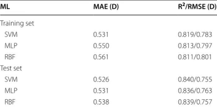
A comparison of three other state-of-the-art ML regres-sors—support vector machines (SVM), multilayer per-ceptron (MLP), and Gaussian Radial Basis Function (RBF)—is shown in Table 7, based on models built with the 75 most important descriptors previously identi-fied for model C. Variation of the ML algorithm could not achieve any consistent improvement of the results obtained with random forests for the training and test sets.
Application of the RF model without DFT‑optimized geometries
The predictive ability of the RF models for a data set in which the DFT-optimized structure is not available was evaluated. The 3D models were generated by CORINA or Dreiding force field methods for the test set, the molecu-lar descriptors were calculated from these 3D structures,
and the previously trained RF models were used to get predictions. The best RF models C, F and MACCS_ DMNBO_DMPEOE had been trained with DFT-optimized
geometries. The MAE increased to 0.78 D, 0.74 D and 0.68 D, respectively, and were essentially independent of the conformer generation method. The same methodol-ogy was followed with two new external data sets (i.e. test set I and test set II), consisting of 200 small organic mol-ecules and a series of 16 2,7-diaryl-[1, 2, 4]triazolo[1,5-a] pyrimidine derivatives, respectively. The predictions were compared to the DM values calculated at the B3LYP/6-31G(d,p) and B3LYP/6-31G(d) levels, respectively, which were retrieved from the literature [2, 8]. The results are presented in Table 8, Figs. 2 and 3.
A MAE of 0.37 D was achieved for test set I with model MACCS_DMNBO_DMPEOE. Although the MAE is higher
for test set II (due to a systematic deviation), the ability to predict trends is remarkable (R2= 0.93), which is
illus-trated with the results for a case of DM cliffs in Fig. 4. Fig. 1 Predicted versus DFT‑calculated DM for the 3368 molecular structures of the external test set. a Predictions obtained with the RF C model trained with 75 descriptors; b predictions obtained with the RF F model trained with 75 descriptors
Table 7 Exploration of different ML algorithms in the prediction of DFT DM using the 75 most important descriptors obtained for model C
Predictions for the training set were obtained with ten‑fold cross‑validation experiments
ML MAE (D) R2/RMSE (D)
Training set
SVM 0.531 0.819/0.783
MLP 0.550 0.813/0.797
RBF 0.561 0.811/0.801
Test set
SVM 0.526 0.840/0.755
MLP 0.531 0.836/0.763
RBF 0.538 0.839/0.757
Table 8 Random forest prediction of the DFT DM for the external test sets I and II
a Test set I comprising 200 molecules calculated at the B3LYP/6‑31G(d,p) level b Test set II comprising 16 molecules calculated at the B3LYP/6‑31G(d) level
Models/test sets MAE (D) R2/RMSE (D)
C/Ia 0.559 0.598/0.782
F/Ia 0.462 0.690/0.656
MACCS_DMNBO_DMPEOE/Ia 0.370 0.752/0.573
C/IIb 1.362 0.938/1.63
F/IIb 1.344 0.944/1.600
Conclusions
ML models trained with 6703 molecules and the respec-tive DMs calculated by density functional theory with B3LYP/31G(d,p) were able to reproduce DFT calcu-lations with MAE up to 0.44 D for an external test set, which is ca. 30% of the MAD in the database. Random forests yielded the best results, and provided a subset of descriptors with high predictive power, notably MACCS fingerprints and the two empirical DMs based on Eq. (1) with point charges calculated by two different methods. The ML approach provides estimations of DMs signifi-cantly closer to DFT calculations than available empirical
methods implementing Eq. (1). The ability to generate 3D structures is outside the scope of this paper; the mod-els here reported have application in the prediction of the DM for a given 3D structure. As this article dem-onstrates, the available 3D structure is only one of the requirements to predict the DM. The application of the ML models (trained with DFT-optimized 3D structures) to molecules with 3D structures generated by empiri-cal methods yielded predictions of the DFT dipoles with worse accuracies for external test sets, but even though, a high correlation was observed (R2= 0.93) between
pre-dicted and calculated DFT DM for a series of 16 mecha-nochromic molecules.
Additional file
Additional file 1:Figure S1. Graphical representation of the DFT‑DM vs. a) DMNBO and b) DMPEOE for the test set. Figure S2. Predicted vs. DFT‑ calculated DM for the 3368 molecular structures of the test set using the model MACCS_DMNBO_DMPEOE.
Authors’ contributions
FP implemented the descriptors, developed and validated the ML models. JAS gathered the data, performed the quantum chemistry calculations, planned and coordinated the work. Both authors contributed to the manuscript write‑ up. Both authors read and approved the final manuscript.
Acknowledgements
We thank ChemAxon Ltd. for access to JChem and Marvin, and Molecular Networks GmbH for access to CORINA.
Competing interests
The authors declare that they have no competing interests.
Availability of data and materials
Geometries and DMs calculated by B3LYP/6‑31G(d,p) for 10,071 organic molecular structures were deposited in the public repository figshare: http://
Fig. 2 Predicted by the model MACCS_DMNBO_DMPEOE versus
DFT‑calculated DM [2] for the 200 molecular structures of the test set I
Fig. 3 Predicted by the model MACCS_DMNBO_DMPEOE versus DFT‑calculated DM [8] for the 16 molecular structures of the test set II
Fig. 4 Illustration of predicted DM values for two molecules of test set II, obtained by the best RF MACCS_DMNBO_DMPEOE model, DFT
dx.doi.org/10.6084/m9.figsh are.57162 46 (DOI not activated while this J. Cheminf. manuscript is under review, meanwhile please use https ://figsh are. com/s/9a430 03365 9a5fc 47213 ).
Consent for publication
Not applicable.
Ethics approval and consent to participate
Not applicable.
Funding
Financial support from Fundação para a Ciência e a Tecnologia (FCT/ MEC) Portugal, under Project PEst‑OE/QUI/UI0612/2013, and Grant SFRH/ BPD/108237/2015 (F.P.) are greatly appreciated. This work was also supported by the Associated Laboratory for Sustainable Chemistry–lean Processes and Technologies–LAQV which is financed by national funds from FCT/MEC (UID/ QUI/50006/2013) and cofinanced by the ERDF under the PT2020 Partnership Agreement (POCI‑01‑0145‑FEDER‑007265).
Publisher’s Note
Springer Nature remains neutral with regard to jurisdictional claims in pub‑ lished maps and institutional affiliations.
Received: 10 January 2018 Accepted: 11 August 2018
References
1. Ioakimidis L, Thoukydidis L, Mirza A, Naeem S, Reynisson J (2008) Bench‑ marking the reliability of QIKPROP. Correlation between experimental and predicted values. QSAR Comb Sci 27(4):445–456
2. Matuszek AM, Reynisson J (2016) Defining known drug space using DFT. Mol Inf 35(2):46–53
3. Sulpizi M, Schelling P, Folkers G, Carloni P, Scapozza L (2001) The rational of catalytic activity of herpes simplex virus thymidine kinase— a combined biochemical and quantum chemical study. J Biol Chem 276(24):21692–21697
4. Adhikari N, Amin SA, Saha A, Jha T (2017) Combating breast cancer with non‑steroidal aromatase inhibitors (NSAIS): understanding the chemico‑ biological interactions through comparative SAR/QSAR study. Eur J Med Chem 137:365–438
5. Wang D, Wu Y, Wang L, Feng J, Zhang X (2017) Design, synthesis and evaluation of 3‑arylidene azetidin‑2‑ones as potential antifungal agents against Alternaria solani Sorauer. Bioorg Med Chem 25(24):6661–6673 6. Wu W, Zhang R, Peng S, Li X, Zhang L (2016) QSPR between molecular
structures of polymers and micellar properties based on block unit auto‑ correlation (BUA) descriptors. Chemom Intell Lab Syst 157:7–15 7. Fong CW (2016) The effect of desolvation on the binding of inhibitors
to HIV‑1 protease and cyclin‑dependent kinases: causes of resistance. Bioorg Med Chem Lett 26(15):3705–3713
8. Wu J, Cheng Y, Lan J, Wu D, Qan S, Yan L, He Z, Li X, Wang K, Zou B, You J (2016) Molecular engineering of mechanochromic materials by pro‑ grammed C‑H arylation: making a counterpoint in the chromism trend. J Am Chem Soc 138(39):12803–12812
9. Dalton LR, Sullivan PA, Bale DH (2010) Electric field poled organic electro‑optic materials: state of the art and future prospects. Chem Rev 110(1):25–55
10. Wojciechowski A, Raposo MMM, Castro MCR, Kuznik W, Fuks‑Janczarek I, Pokladko‑Kowar M, Bures F (2014) Nonlinear optoelectronic materials formed by push‑pull (bi)thiophene derivatives functionalized with di(tri) cyanovinyl acceptor groups. J Mater Sci: Mater Electron 25(4):1745–1750 11. Sliwoski G, Kothiwale S, Meiler J, Lowe EW Jr (2014) Computational meth‑
ods in drug discovery. Pharmacol Rev 66(1):334–395
12. Nakata M, Shimazaki T (2017) PubChemQC project: a large‑scale first‑ principles electronic structure database for data‑driven chemistry. J Chem Inf Model 57(6):1300–1308
13. Pyzer‑Knapp EO, Suh C, Gomez‑Bombarelli R, Aguilera‑Iparraguirre J, Aspuru‑Guzik A (2015) What is high‑throughput virtual screening?
A perspective from organic materials discovery. Annu Rev Mater Res 45:195–216
14. Rajan K (2015) Materials informatics: the materials “Gene” and big data. Annu Rev Mater Res 45:153–169
15. Cheng L, Assary RS, Qu X, Jain A, Ong SP, Rajput NN, Persson K, Curtiss LA (2015) Accelerating electrolyte discovery for energy storage with high‑ throughput screening. J Phys Chem Lett 6(2):283–291
16. Faber FA, Hutchison L, Huang B, Gilmer J, Schoenholz SS, Dahl GE, Vinyals O, Kearnes S, Riley PF, von Lilienfeld OA (2017) Prediction errors of molecular machine learning models lower than hybrid DFT error. J Chem Theory Comput 13(11):5255–5264
17. Mehata MS, Singh AK, Sinha RK (2016) Experimental and theoretical study of hydroxyquinolines: hydroxyl group position dependent dipole moment and charge‑separation in the photoexcited state leading to fluorescence. Methods Appl Fluoresc 4(4):045004
18. Bianco A, Ferrari G, Castagna R, Rossi A, Carminati M, Pariani G, Tom‑ masini M, Bertarelli C (2016) Light‑induced dipole moment modula‑ tion in diarylethenes: a fundamental study. Phys Chem Chem Phys 18(45):31154–31159
19. Rai BK, Bakken GA (2013) Fast and accurate generation of ab initio quality atomic charges using nonparametric statistical regression. J Comput Chem 34(19):1661–1671
20. Ramakrishnan R, Dral PO, Rupp M, von Lilienfeld OA (2014) Quantum chemistry structures and properties of 134 kilo molecules. Sci Data 1:140022
21. Pereira F, Xiao K, Latino DARS, Wu C, Zhang Q, Aires‑de‑Sousa J (2017) Machine learning methods to predict density functional theory B3LYP energies of HOMO and LUMO orbitals. J Chem Inf Model 57(1):11–21 22. Irwin JJ, Sterling T, Mysinger MM, Bolstad ES, Coleman RG (2012)
ZINC: a free tool to discover chemistry for biology. J Chem Inf Model 52(7):1757–1768
23. Blum LC, Reymond J‑L (2009) 970 million druglike small molecules for virtual screening in the chemical universe database GDB‑13. J Am Chem Soc 131(25):8732–8733
24. Schmidt MW, Baldridge KK, Boatz JA, Elbert ST, Gordon MS, Jensen JH, Koseki S, Matsunaga N, Nguyen KA, Su SJ, Windus TL et al (1993) General atomic and molecular electronic‑structure system. J Comput Chem 14(11):1347–1363
25. Gordon MS, Schmidt MW (2005) Advances in electronic structure theory: GAMESS a decade later. In: Dykstra CE, Frenking G, Kim KS, Scuseria KS (eds) Theory and applications of computational chemistry: the first forty years. Elsevier, Amsterdam, pp 1167–1189
26. Becke AD (1993) A new mixing of Hartree–Fock and local density‑func‑ tional theories. J Chem Phys 98(2):1372–1377
27. Becke AD (1993) Density‑functional thermochemistry. III. The role of exact exchange. J Chem Phys 98(7):5648–5652
28. Latino DARS, Aires‑de‑Sousa J (2017) Geometries and dipole moments calculated by B3LYP/6‑31G(d,p) for 10071 organic molecular structures. In: figshare. http://dx.doi.org/10.6084/m9.figsh are.57162 46
29. Zhang Q, Zheng F, Fartaria R, Latino DARS, Qu X, Campos T, Zhao T, Aires‑ de‑Sousa J (2014) A QSPR approach for the fast estimation of DFT/NBO partial atomic charges. Chemom Intell Lab Syst 134:158–163 30. Selzer P, Ertl P (2005) Identification and classification of GPCR ligands
using self‑organizing neural networks. QSAR Comb Sci 24(2):270–276 31. Yap CW (2011) PaDEL‑descriptor: an open source software to calculate
molecular descriptors and fingerprints. J Comput Chem 32(7):1466–1474 32. Hall MA, Smith LA (1999) Correlation‑based feature selection for machine
learning. PhD Diss. The University of Waikato
33. Hall M, Frank E, Holmes G, Pfahringer B, Reutemann P, Witten IH (2009) The WEKA data mining software: an update. SIGKDD Explor Newsl 11(1):10–18
34. Breiman L (2001) Random forests. Mach Learn 45(1):5–32
35. Svetnik V, Liaw A, Tong C, Culberson JC, Sheridan RP, Feuston BP (2003) Random forest: a classification and regression tool for compound clas‑ sification and QSAR modeling. J Chem Inf Comput Sci 43(6):1947–1958 36. R: A language and environment for statistical computing. In: Team RDC (Ed) R Foundation for Statistical Computing. Vienna, Austria; 2014. http:// www.R‑proje ct.org
38. Cortes C, Vapnik V (1995) Support‑vector networks. Mach Learn 20(3):273–297
39. Chang C‑C, Lin C‑J (2011) Libsvm: a library for support vector machines. ACM Trans Intell Syst Technol. https ://doi.org/10.1145/19611 89.19611 99