Multi-Cloud Provisioning and Load Distribution for Three-Tier
Applications
NIKOLAY GROZEV, University of Melbourne, Australia
RAJKUMAR BUYYA, University of Melbourne, Australia
Cloud data centres are becoming the preferred deployment environment for a wide range of business appli-cations, as they provide many benefits compared to private in-house infrastructure. However, the traditional approach of using a single cloud has several limitations in terms of availability, avoiding vendor lock-in and providing legislation compliant services with suitable Quality of Experience (QoE) to users worldwide. One way for Cloud clients to mitigate these issues is to use multiple clouds (i.e. a Multi-Cloud). In this paper we introduce an approach for deploying 3-tier applications across multiple clouds in order to satisfy their key non-functional requirements. We propose adaptive, dynamic and reactive resource provisioning and load distribution algorithms, which heuristically optimise the overall cost and the response delays, without vi-olating essential legislative and regulatory requirements. Our simulation with realistic workload, network and cloud characteristics shows that our method improves the state of the art in terms of availability, regu-latory compliance and QoE with acceptable sacrifice in cost and latency.
Categories and Subject Descriptors: D.2.11 [Software Engineering]: Software Architectures; C.2.4 [Computer-Communication Networks]: Distributed Systems
General Terms: Performance, Legal Aspects, Experimentation
Additional Key Words and Phrases: Cloud Computing, Multi-Cloud, 3-Tier Applications, Autoscaling, Load Balancing
1. INTRODUCTION
Cloud computing is a disruptive IT paradigm, which changes the way businesses oper-ate. Instead of owning, maintaining and administering their own infrastructure, busi-nesses can now dynamically rent resources on demand just as they need them [Buyya et al. 2009], [Mell and Grance 2011]. This allows them to avoid upfront investments in infrastructure that may not fit their dynamic needs at all times being either under or over-utilised. Moreover, enterprises can now eliminate activities like infrastructure maintenance and administration thus focusing on their core business operations.
The standard model of consuming a cloud service is when a client uses resources within a single cloud. However, this poses several challenges for cloud clients. Firstly, a data centre outage can leave clients without access to resources as exemplified by the outages of several major vendors [Amazon 2014e], [Amazon 2014f], [Google 2014], [Mi-crosoft 2014]. As to Berkeley’s report, cloud service unavailability is the greatest in-hibitor to cloud adoption [Armbrust et al. 2009]. Secondly, interactive online appli-cations (e.g. 3-tier systems) usually have network latency constraints. A single data Nikolay Grozev and Rajkumar Buyya are with the Cloud Computing and Distributed Systems (CLOUDS) Laboratory, Department of Computing and Information Systems, The University of Melbourne, Parkville, VIC 3010, Australia.
Email: [email protected], [email protected]
Permission to make digital or hard copies of part or all of this work for personal or classroom use is granted without fee provided that copies are not made or distributed for profit or commercial advantage and that copies show this notice on the first page or initial screen of a display along with the full citation. Copyrights for components of this work owned by others than ACM must be honored. Abstracting with credit is per-mitted. To copy otherwise, to republish, to post on servers, to redistribute to lists, or to use any component of this work in other works requires prior specific permission and/or a fee. Permissions may be requested from Publications Dept., ACM, Inc., 2 Penn Plaza, Suite 701, New York, NY 10121-0701 USA, fax+1 (212) 869-0481, or [email protected].
c
2014 ACM 1556-4665/2014/06-ART $15.00 DOI:http://dx.doi.org/10.1145/0000000.0000000
centre cannot serve users distributed worldwide with adequate latency. Lastly, many businesses that operate across national boundaries need to comply with different reg-ulations in terms of privacy, security and data location. This is of special importance for applications dealing with sensitive data (e.g. in the banking or e-health domains), which are often required to use data centres within a given territorial jurisdiction, when serving some customers [Bowen 2011]. It is unlikely that a single data centre will comply with the constraints of all targeted jurisdictions.
To overcome these issues, researchers and practitioners have envisioned the usage of multiple clouds. A Multi-Cloud is a type of Inter-Cloud where clients utilise multi-ple clouds without relying on any interoperability functionalities immulti-plemented by the providers [Ferrer et al. 2012], [Petcu 2013], [Grozev and Buyya 2012]. Application de-ployment across clouds has recently attracted interest resulting in the emergence of at least 20 projects facilitating cross-cloud deployment [Grozev and Buyya 2012]. Case studies by IBM [2013] and ebay[2014] have demonstrated how 3-tier interactive ap-plications can utilise multiple data centres to provide better availability and QoE and to quickly adapt to changes in the demand.
Unfortunately, transitioning existing applications to Clouds or Multi-Clouds is not straightforward. A Cloud is not merely a deployment environment, where existing soft-ware solutions can be transferred. It introduces novel characteristics not existing in traditional in-house deployment environments like seemingly endless resource pool and the risk of an unpredictable outage in external infrastructure [Varia 2011]. Hence software applications need to be more scalable and fault tolerant so they can dynami-cally adapt to workload fluctuations by adequately allocating and releasing computing resources and autonomously and timely address infrastructure failures. Software en-gineers need to design for the Cloud, not only to deploy in the Cloud. This is even more important when using multiple data centres situated in different legislative domains, constructed with different hardware, network and software components and prone to different environmental risks.
The key contributions of this work are (i) a design approach for interactive 3-tier Multi-Cloud applications and (ii) adaptive dynamic provisioning and autonomous workload redirection algorithms ensuring imperative constraints are met with min-imal sacrifice in cost and QoE. We focus on the 3-tier architectural pattern, as it is pervasive and many enterprise systems follow it. Our approach does not modify the 3-tier pattern itself, but introduces additional components managing the cross-cloud resource provisioning and workload distribution. This is essential as it allows the mi-gration of existing applications to a Multi-Cloud environment. Also new Multi-Cloud 3-tier applications can be developed using the plethora of existing architectural frame-works thus leveraging proven technologies and existing know-how. The newly intro-duced components facilitate the implementation of 3-tier systems which observe: (i) increased availability and resilience to cloud infrastructure failure (ii) legislation and regulation compliance (iii) high QoE and (iv) cost efficiency.
The rest of the paper is organised as follows: In Section 2 we provide an overview of the related works and compare them to ours. Section 3 details the targeted class of applications. Section 4 outlines our architecture. Section 5 motivates and details our algorithms for load balancing, autoscaling and cloud selection. Our experimental settings and results are discussed in Section 6. In the final Section 7, we conclude the paper and define pathways for future work.
2. RELATED WORK
There have been significant efforts in the development of Multi-Cloud open source li-braries for different languages like JClouds [2014], Apache LibCloud [2014b], Apache DeltaCloud [2014a], SimpleCloud [2012] and Apache Nuvem [2014c]. All of them
pro-vide a unified API for the management of cloud resources (e.g. VMs and storage), so that software engineers do not have to program against the specifics of each vendor’s API. While not providing application brokering (consisting of provisioning and schedul-ing) themselves, these libraries can be instrumental in the development of new cross-cloud brokering components. Similarly, services like RightScale [2014], Enstratius (for-merly enStratus) [2014], Scalr [2014] and Kaavo [2014] only provide unified user in-terface, APIs and tools for managing multiple clouds and it is the clients’ responsibility to implement appropriate provisioning and scheduling.
Apart from these Multi-Cloud libraries and services, the OPTIMIS [Ferrer et al. 2012], Contrail [Carlini et al. 2012], mOSAIC [Petcu et al. 2011], MODA-Clouds [Ardagna et al. 2012] and STRATOS [Pawluk et al. 2012] projects also facil-itate Multi-Cloud application deployment. In all of these projects the geographical lo-cations of the serving data centres cannot be considered. Thus, often it is not possible to implement legislation aware application brokering. In contrast, in our approach the Entry Points and Data Centre Controllayers enable legislation compliant user rout-ing to eligible clouds through a process calledmatchmaking broadcast.Secondly, all of these projects only manage resource allocation and software component deployment, and none of them facilitates the distribution of the incoming workload to the allocated resources. Their components are only concerned with resource provisioning and set-up and do not deal with the load distribution and autoscaling of the application once it is installed. In contrast, in this work we manage the incoming workload and dynamically provision resources accordingly through the components of theEntry PointsandData Centre Controllayers.
Furthermore, these projects are SLA-based, which means the application brokering is specified in a Service Level Agreement (SLA) using a declarative formalism. The Cloud Standards Customer Council (CSCC) discusses in a technical report that SLAs currently offered by cloud providers are immature [2012]. Thus, to achieve flexible ap-plication brokering these approaches rely on advances in the currently adopted SLA practices, or the introduction of new brokering components that can interpret novel SLA formalisms. In contrast, our approach directly manages the underlying provision-ing and the mappprovision-ing of workload to resources, without relyprovision-ing on advances in SLA specifications, and thus it is applicable right away.
Cloud services like Route 53 [Amazon 2014c] and AWS Elastic Load Balancer (ELB) [Amazon 2014d] can distribute incoming users to servers in multiple data cen-tres using standard load balancing techniques. AWS ELB can distribute workload among servers located in a single or multiple AWS availability zones, but cannot direct users to clouds of other providers. Route 53 is Amazon’s Domain Name System (DNS) web service. It supports Latency Based Routing (LBR), which redirects incoming users to the AWS region with the lowest latency. Both Route 53 and ELB do not consider ap-plications’ regulatory requirements when selecting a data centre site. Moreover, they do not consider the cost and the degree of utilisation of the employed within a data centre resources. In contrast, our approach for directing users to cloud sites accounts for all these aspects.
3. PRELIMINARIES
By definition an interactive 3-tier application has three layers [Fowler 2003], [Ramirez 2000], [Aarsten et al. 1996]:
—Presentation Layer— represents the user interface.
—Business/Domain Layer— features the main business logic. Accesses and modifies
the data layer.
The presentation layer executes at the end user’s site, not in the back-end servers, and thus we will not consider it. The domain layer consists of one or several application servers (AS). In Infrastructure as a Service (IaaS) cloud environments they are hosted in separate VMs. The data layer consists of one or several database (DB) servers. In a Multi-Cloud environment this software stack is replicated across all used cloud data centres. Clients arrive at one or several entry points, from where they are redirected to the appropriate data centre to serve them.
The domain layer within a data centre can scale horizontally by adding more AS VMs. For a given application, within a data centre there is a load balancer, which distributes the incoming requests to the AS servers. Every request arrives at the load balancer, which selects the AS to serve it. There are two types of 3-tier applications in terms of the domain layer design — statefulandstateless. Stateful applications keep session data (e.g. shopping carts and user meta-data) in the memory of the assigned AS server. Hence they require sticky load balancing, which ensures all requests of a session are routed to the same server. Stateless applications do not keep any state/data in memory and therefore their requests can be routed to different AS servers.
The data layer often becomes the performance bottleneck because of requirements for transactional access and atomicity. This makes it hard to scale horizontally. As to the famous CAP theorem [Brewer 2000], [Brewer 2012] a distributed database architect should balance between persistent storage consistency, availability and par-tition tolerance. The field of distributed horizontally scaling databases has been well explored in recent years. For example Cattell [2010] surveyed over 20 novel NoSQL and NewSQL distributed database projects. Traditional techniques like replication, caching and sharding also allow for some level of horizontal scalability.
The eligible data caching and replication strategies are very much application spe-cific and it is impossible to incorporate them within a general framework encompassing all 3-tier applications. In other words the right balance between the CAP (consistency, availability and partition tolerance) requirements is domain inherent. For example one application may require that data is not replicated across legislative regions, while an-other may allow it in order to achieve better availability. Therefore in this work we do not deal with the application specific data deployment. We investigate flexible pro-visioning and load distribution provided the data is already deployed with respect to the application specific CAP requirements. It is the system architect’s responsibility to design the data layer in a scalable way obeying all domain specific legislation rues so that it can be accessed quickly from the domain layer. This is a reasonable con-straint, as database design is usually the first step in a 3-tier system design and it often serves other applications (e.g. reporting and analytics) as well. Our approach en-sures that once the data is deployed appropriately, users will be redirected accordingly and enough processing capacities will be present in the AS layer.
4. OVERALL ARCHITECTURE 4.1. Architectural Components
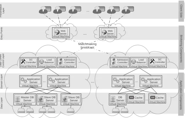
Figure 1 depicts the proposed architecture. We augment the traditional 3-tier archi-tectural pattern with two additional layers of components:
—Entry Point Layer — responsible for redirecting incoming users to an appropriate cloud data centre to serve them.
—Data Centre Control Layer— responsible for: (i) providing information to theentry point layerregarding the suitability of a data centre for a given user, (ii) monitoring and scaling of the provisioned resources within a data centre and (iii) directing the incoming requests.
... ... ... ... Matchmaking broadcast Virtual Machine Web Server Virtual Machine Application Server Virtual Machine Web Server Virtual Machine Application Server Virtual Machine Application Server Virtual Machine Application Server Admission Controller Load Balancer Virtual Machine DC
Controller BalancerLoad
Virtual Machine Virtual Machine Application Server D at a La ye r D om ai n La ye r D at a C en tr e C on tr ol L ay er E nt ry P oi nt s B ro ke rin g C o m po ne nt s DC Controller Virtual Machine Admission Controller Virtual Machine Load Balancer Virtual Machine DC Controller Virtual Machine Admission Controller Virtual Machine Load Balancer Virtual Machine DC Controller Virtual Machine Admission Controller Virtual Machine Web Server Virtual Machine Virtual Machine Master DB Server Virtual Machine Slave DB Server Virtual Machine DB
Server Virtual MachineCache ... Virtual Machine Slave DB Server ... P re se nt at io n La ye r Virtual Machine Master DB Server Virtual Machine Slave DB Server Virtual Machine DB Server Virtual Machine Cache Cache Virtual Machine ... A pp lic at io n C om po n en ts C lie n t S id e
Fig. 1. Overall layered architecture. The Brokering components mange the system’s provisioning and
work-load distribution, while a standard 3-tier software stack serves the end users.
The Entry Point Layer consists of one or several VMs, which can be deployed in several data centres for better resilience. When users come to the system, they are initially served at anentry point VM. Based on the users’ location, identity, and in-formation about each data centre, the entry point selects an appropriate cloud and redirects the user to it. After this, the user is served within the selected data centre and has no further interaction with theentry point. We emphasise that the cross-cloud interactions betweenentry pointsandadmission controllershappen only once, imme-diately after user arrival, and hence does not result in further communication delay as the user is being served.
At first glance anentry pointcan be likened to a standard load balancer, as it redi-rects users to serving data centres. However, standard load balancers redirect each user request, whileentry points redirect users only upon arrival. Furthermore,entry pointscollaborate with theadmission controllersto implement cloud selection respect-ing legislative, data location, cost and QoE requirements, which is not implemented in standard load balancers.
In each data centre theData Centre Control Layerconsists of three VMs:
—Admission Controller— decides whether a user can be served within this data centre and provides an estimation of the potential cost for serving him/her. Upon request, it provides feedback to theentry pointVMs to facilitate their choice of a data centre for a user.
—Load Balancer— the standard load balancer component from the 3-tier reference architecture. We consider it as a logical part of theData Centre Control Layer, since it redirects requests to the application servers.
Loop - user is served
Admission controllers of all data centres :Entry Point redirect to redirect to cloud selection VMs deployed within the selected data centre
End User Data Centre Selection
send requests to the system
:DB Server
authenticate
:Admission Controller :AS Server
respond to user accessdata admission request
:Load Balancer
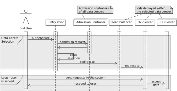
Fig. 2. Component Interaction. Cloud site selection happens once, upon the user arrival. Subsequent
re-quests are handled within the selected data centre.
—DC Controller — responsible for observing the performance utilisation of the run-ning AS servers, and reactively shutting down or starting AS VM instances to meet resource demands at minimal cost.
In principal theDC Controllerand theLoad BalancerVMs may be replaced by ser-vices like Amazon Auto Scaling [2014a] and AWS Elastic Load Balancer (ELB) [2014d]. Nevertheless, not all cloud providers have such services. Even if a provider offers auto scaling services, it is often not possible (unlike Amazon Auto Scaling) to monitor cus-tom performance metrics - e.g. number of live application sessions. Moreover, in Sec-tion 5 we introduce novel algorithms for load balancing and autoscaling which in con-junction reduce cost and the probability of server overload. These are not implemented by current cloud providers and hence, for generality, we will consider the usage of sep-arate VMs for these purposes.
4.2. Component Interaction
Figure 2 depicts the interaction between components upon user arrival. In the first phase, the brokering components select an appropriate cloud site for the user, based on his/her identity. As a first step, the user authenticates to one of theentry points. At this point, theentry pointhas the user’s identity and geographical location (extracted from the IP address). As a second step, theentry pointbroadcasts the user’s identifier to the admission controllersof all data centres. We call this stepmatchmaking broadcast.
There are no restrictions on the location of theentry points. Ideally, they should be positioned in a way which minimises the network latency effects during the match-making broadcast. One reasonable approach is to deploy each entry point in one of the used clouds, given that the clouds are already selected in a way which serves the expected user base with adequate latency.
Within each data centre, the admission controllerchecks if the persistent data for this user is present. Additionally each admission controller implements application specific logic to determine which users can be served in the data centre based on the regulatory requirements. Theadmission controllersrespond to theentry pointwhether the user’s data is present and if they are allowed (in terms of legislation and
regula-tions) to serve the user. In the response, they also include information about the costs within the data centre.
Based on theadmission controllers’responses, theentry pointselects the data cen-tre to serve the user and redirects him/her to the load balancer deployed within it. Theentry pointfilters all clouds which have the user’s data and are eligible to serve him/her. If there is more than one such cloud, theentry pointselects the most suitable with respect to network latency and pricing. If no cloud meets the data location and legislative requirements the user is denied service.
After a data centre is selected the user is served by the AS and DB servers within the chosen cloud as prescribed by the standard 3-tier architecture. He or she does not have any further interaction with the brokering components. Hence we consider that AS servers deployed in a data centre can only access DB servers in the same data centre. This is a reasonable constraint, as often there is no SLA about the network speed and latency between data centres, and thus cross-cloud data access can lead to performance issues. Furthermore, transferring persistent data across the public Internet may be a breach of the legislation and policy requirements of many applications.
5. PROVISIONING AND WORKLOAD MANAGEMENT 5.1. Scalability Within a Cloud
Currently, the practices for load balancing among a dynamic number of VMs in a cloud environment and among a fixed number of physical servers are the same - e.g. round robin or some of its adaptations. When using physical servers, one usually tries to distribute the load so that the servers are equally loaded and all sessions are served equally well. In a cloud environment, if the number of AS VMs is insufficient, new ones can be provisioned dynamically. Similarly, if there are more than enough allocated AS VMs, some of them could be stopped to reduce costs. If the load of a stateful application is equally distributed among underutilised VMs, then no VM can be stopped without failing the sessions served there.
This is not an impediment for stateless applications, as sessions are not bound to servers and hence VMs can be stopped without causing service disruption. Thus, stan-dard load balancing techniques like weighted round robin or “least connection” can be effective. However, in the case of stateful sessions, in order to stop an AS VM one needs to make sure it does not serve any sessions. One approach is to transfer all ses-sions from an AS VM to another one before shut-down. However, this is not straight-forward, as active sessions together with their states need to be transferred without service interruption. A better approach is to balance the incoming workload in a way, which consolidates the sessions in as few servers as possible without violating the QoS requirements. This results in a maximum number of stoppable (i.e. not serving any sessions) servers. In essence, if the load balancer packs as many sessions as possible (without causing overload) to a few servers, then the number of stoppable servers (not serving any sessions) will be maximal.
This idea is implemented in Algorithm 1. It defines asticky load balancing policy, and thus after the first session’s request is assigned to a server all successive ones are assigned to it as well. It takes as input, the newly arrived session si, the list
of already deployed AS servers V Mas and two ratio numbers in the interval (0,1)
-the CPU and RAM thresholds thcpu and thram. As a first step in the algorithm, we
sort the available AS VMs in a descending order with respect to their CPU utilisa-tion. Then we assign the incoming session to the first VM in the list, whose CPU and RAM utilisations are below thcpu and thram respectively and whose input and
out-put TCP network buffers/queues are not becoming overloaded. These buffer sizes are denoted by the Recv-Q and Send-Q values returned by thenetstatcommand. To
sim-ALGORITHM 1:Load Balancing Algorithm
input :si,thcpu,thram,V Mas
1 sortDescendinglyByCPUUtilisation(V Mas); 2 hostV M←−last element ofV Mas;
3 forvmi∈V Masdo
4 vmcpu←−CPU utilisation ofvmi; 5 vmram←−RAM utilisation ofvmi;
6 ifvmcpu< thcpuandvmram< thramand !networkBuffersOverloaded()then 7 hostV M←−vmi;
8 break;
9 end
10 end
11 assignSessionTo(s,hostV M)
plify the algorithm’s definition we have extracted this logic in a new boolean function
networkBuf f ersOverloaded(). It simply checks if there is a TCP socket for which any
of the ratios of the Recv-Q and Send-Q values to the maximum capacities of those queues is greater than 0.9. If there is no such server, the session is assigned to the least utilised one (line 2). An obvious postcondition of the algorithm is that a newly ar-rived session is assigned to the most utilised in terms of CPU server, whose CPU and RAM utilisations are under the thresholds. If there is no such server - the one with the least utilised CPU is used. By increasing the thresholds, we can achieve better consol-idation of sessions at the expense of a higher risk of CPU or RAM contention, which may result in lower response time. On the contrary, when the thresholds are lower, the overall number of underutilised VMs will be higher. Therefore reasonable values for these thresholds are the autoscaling triggers (used by our autoscaling algorithm), which define if a server is overloaded.
TheDC controller is responsible for adjusting the number of AS VMs accordingly. This implementation of the load balancer (Algorithm 1) allows theDC controller to stop AS VMs which serve no sessions. TheDC controlleris also responsible for instan-tiating new AS VMs when needed. Algorithm 2 details how this can be done when using on-demand VM instances. This algorithm is periodically executed every ∆ sec-onds to ensure the provisioned resources match the demand at all times. The input parameters of the algorithm are:
—tcur — the current time of the algorithm call;
—tgrcpu— CPU trigger ratio in the interval(0,1);
—tgrram— RAM trigger ratio in the interval(0,1);
—V Mas— list of currently deployed AS VMs;
—n— number of over-provisioned AS VMs to cope with sudden peaks in demand; —∆— time period between algorithm repetitions.
If an AS VM’s CPU or RAM utilisation exceeds respectively tgrcpu and tgrram or
some of its input/output TCP network buffers is becoming overloaded, we call this server overloaded. In the beginning of Algorithm 2 (lines 1-11) we inspect the statuses of all available AS VMs and note if they are overloaded or free (i.e. not serving any sessions).
In an online application, the resource demand can raise unexpectedly in the time periods between two subsequent executions of the scaling algorithm. Moreover, booting and setting up new AS VMs is not instantaneous and can take up to a few minutes depending on the underlying infrastructure. Hence, resources cannot be provisioned instantly in response to the increased workload. If the workload spike is significant,
ALGORITHM 2:Scale Up/Down Algorithm
input :tcur,tgrcpu,tgrram,V Mas,n,∆
1 nOverloaded←−0;
2 listF reeV ms←−empty list;
3 forvm∈V Mas; // Inspect the status of all AS VMs 4 do
5 vmcpu←−CPU utilisation ofvm; 6 vmram←−RAM utilisation ofvm;
7 ifvmcpu>=tgrcpuorvmram>=tgrramor networkBuffersOverloaded()then
8 nOverloaded←−nOverloaded+ 1;
9 else ifvmiserves no sessionsthen
10 listF reeV ms.add(vm); 11 end
12 end
13 nF ree←−length oflistF reeV ms; 14 nAS←−length ofV Mas;
15 allOverloaded←−nOverloaded+nF ree=nASandnOverloaded >0;
16 ifnF ree≤n; // Provision more VMs
17 then 18 nV msT oStart←−0; 19 ifallOverloadedthen 20 nV msT oStart←−n−nF ree+ 1; 21 else 22 nV msT oStart←−n−nF ree 23 end 24 launchnV msT oStartAS VMs 25 else 26 nV msT oStop←−0; // Release VMs 27 ifallOverloadedthen 28 nV msT oStop←−nF ree−n; 29 else 30 nV msT oStop←−nF ree−n+ 1 31 end
32 sortAscendinglyByBillingTime(listF reeV ms); 33 fori= 1tonV msT oStopdo
34 billT ime←−billing time oflistF reeV ms[i]; 35 ifbillT ime−tcur<∆then
36 terminatelistF reeV ms[i];
37 else
38 break
39 end
40 end 41 end
this can result in server overload and performance degradation. One solution is to over-provision AS VMs, so that unexpected workload spikes can be handled. The n
input parameter of the algorithm denotes exactly that — how many AS VMs should be over-provisioned to cope with unexpected demand.
As a postcondition of the algorithm execution, there should be at leastn+ 1free AS VMs if all other AS VMs are overloaded, or notherwise. For example in the special case whenn = 0, one AS VM is provisioned only if all others are overloaded. This is ensured by lines 16-24 of the algorithm.
Similarly, to avoid charges some over-provisioned VMs should be stopped whenever their number exceedsn. However, it is not beneficial to terminate a running VM ahead of its next billing time. It is better to keep it running until its billing time, in order to reuse it if resources are needed again. This is ensured by lines 25-40 of the algorithm. Firstly, we sort the free VMs in ascending order with respect to their next billing time. Next, we iterate through the excessively allocated VMs and terminate only those for which the next billing time is earlier than the next algorithm execution time.
Lastly, in the previous discussion we assumed that the application is stateful - i.e. it maintains contextual user information in the memory of the AS server. For scalability reasons many applications are stateless, or they store session state in an external in-memory cache like Amazon ElastiCache [2014b]. Algorithm 2 can handle this type of applications as well by considering each AS server to be assigned 0 sessions at all times. This is reflective of the main characteristic of stateless applications that each request can be served on a different server, as no session state is kept in the servers’ memory. Consequently in the algorithm all AS servers which are not overloaded will be considered free (lines 9-11) and will be viable for termination. Therefore our approach encompasses both stateful and stateless applications.
5.2. Data Centre Selection
We can largely classify the requirements for data centre selection as constraints and objectives. Constraints should not be violated under any circumstances. In this work we consider the following constraints: (i) users should be served in data centres which are compliant with the regulatory requirements and (ii) users should be served in data centres containing their data in the application’s data layer. The system should prefer to deny service than to violate these constraints. In contrast, the system can continue to serve a user even if an objective is not optimised. We consider the following objectives: (i) cost minimisation and (ii) latency minimisation. In other words, upon a user arrival theentry pointextracts the data centres which satisfy the constraints and selects the most suitable among them in terms of latency and cost.
While cost minimisation is a natural goal of cloud clients, it should not be pursued at the expense of end user Quality of Experience (QoE) and hence we must balance between the two objectives. The maximum acceptable latency between users and the data centres can be considered as a part of the application’s SLA. Thus we can choose the optimal data centre in terms of cost, whose network latency is less than the prede-fined in the SLA one.
Algorithm 3 implements this idea and details the data centre selection procedure. The algorithm selects clouds for multiple users at once. Hence, users arriving at the system at approximately the same time can be dispatched to serving clouds in batch thus avoiding excessive cross cloud communication. The input parameters of the algo-rithm are:
—users— identifiers of the users, for which theentry pointshould select a cloud.
—timeout — period after which if a data centre’s admission controller has not
re-sponded it is discarded.
—clouds — a list of the used data centres. For each of them, we can obtain the IP
addresses of theadmission controllerand theload balancer.
—latencySLA— SLA for the network latency between a user and the serving data
cen-tre.
In the beginning of the algorithm (lines 1-4) theentry pointasynchronously broad-casts all users’ identifiers to the clouds’admission controllers. After that theentry point waits until all contacted admission controllersrespond or the timeout period elapses
ALGORITHM 3:Cloud Site Selection Algorithm
input :users,timeout,clouds,latencySLA
// Broadcast users’ data to admission controllers 1 forci∈cloudsdo
2 aci←−IP address ofci’sadmission controller; 3 send toaciusers’ identifier;
4 end
5 waittimeoutseconds or until all clouds respond; 6 forui∈usersdo
7 cloudsaccept←−clouds eligible to serveui; 8 sortAscendinglyByPrice(cloudsaccept); 9 selectedCloud←−null;
10 selectedLatency←−+∞; 11 forci∈cloudsacceptdo
12 latency←−latency betweenuandci; 13 iflatency < latencySLAthen
14 selectedCloud←−ci; 15 break;
16 else ifselectedLatency > latencythen
17 selectedCloud←−ci; 18 selectedLatency←−latency;
19 end
20 end
21 ifselectedCloud=nullthen 22 Deny Service;
23 else
24 lb←−IP ofload balancerinselectedCloud; 25 redirectutolb;
26 end 27 end
(line 5). At this stage unresponsive clouds whoseadmissions controllersfail to respond within the timeout are discarded.
For each user, the response of the clouds’admission controllersincludes: (i) a boolean value, whether the cloud is eligible to serve the user and (ii) an estimation of the cost for serving a user. Based on this input, for every user theentry pointretains the clouds eligible to serve him/her (line 7). If no eligible cloud is present the user is denied service. Otherwise, the cloud which has the smallest cost and provides latency below the SLA requirement is selected (lines 9-20). If there is no eligible cloud meeting the network latency SLA - the one with the lowest network latency to the user is selected (lines 16-19).
Note that the decision if a cloud site is eligible for a given user is application specific. For some applications with no additional privacy, security and legislation requirements all clouds may be eligible for all users. In others, certain users will have to be served within a specific legislative domain or within certified data centres based on their nationality. We assume that this application specific eligibility logic is implemented in admission controllersby application developers.
Algorithm 3 uses the network latency between the end user and the prospective serv-ing data centres. Hence theentry pointneeds to evaluate the latencies between them based on their IP addresses. By latency we denote only the network latency. We do not try to estimate the entire response time, consisting of network and server delays. We
argue this simplification does not reduce the generality of our approach, because for an interactive 3-tier application the server delays should be small and similar in all clouds provided there is no significant resource contention. In this case the variable part of the overall delay is the network latency. In Algorithm 2 we make sure the domain layer scales horizontally and enough resources are present at all times. If contention indeed occurs within a cloud site, because of either non-scalable DB layer or inappropriate choice of parameters for Algorithm 2, then we provide a back-off mechanism through the cost estimation, as discussed below. Hence we minimise the probability of resource contention within the Multi-Cloud set-up and therefore servers’ delays should be small and similar in all cloud sites.
An approximation of the network latency can be achieved in two steps. Firstly we can identify the geographical locations (longitude and latitude) of the user and a given cloud based on their IP addresses. For this we use the GeoLite [2014] database, map-ping IP addresses to geospatial coordinates. As a second step, we compute the la-tency between a user and a cloud based on the extracted coordinates by using the PingER [2014] service. PingER is an end-to-end Internet performance measurement (IEPM) project, which constantly records the network metrics between more than 300 hosts positioned worldwide. The geospatial coordinates of each host are provided. To approximate the latency between a user and a cloud, we select the 3 pairs of PingER hosts that are closest to the user and the cloud respectively, and define the latency as a weighted sum of the 3 latencies between the hosts in these 3 pairs. The weights are defined proportionally to the proximity of the hosts to the user and the cloud. To com-pute the distance between the geospatial positions we use the well known Vincenty’s formulae. The data from both GeoLite and PingER can be downloaded and used of-fline. If latest up-to-date Internet performance data is needed it can be periodically downloaded and updated automatically.
The last missing piece of information is the cost evaluation for serving a user by a cloud (used in line 8), performed by theadmission controllers. The difficulty here is to define a unified cost evaluation for different clouds, with different pricing policies and different VM types and performance.
Firstly, if the application’s infrastructure within a data centre is overloaded and it should not accept further users, it returns +∞as a cost estimation. One reason for an overload may be a lack of scalability in the DB layer. As discussed, it can be hard to scale horizontally, and given significant workload can be easily overloaded. Another reason may be a bottleneck in the data centre infrastructure - for example an internal network congestion may threaten to slow down the application’s inter-tier communica-tion. This could be easily detected in the case of a private data centre. In a public data centre obtaining such information may be more difficult, as the cloud provider would have to expose such internal performance data to its clients. By returning +∞cost to theentry pointtheadmission controllerensures that users are sent to this cloud only as a last resort. Henceadmission controllersuse the cost as a back-off mechanism.
As a first step in session cost estimation, we definep(vmi)to be the price per minute
of a virtual machinevmi. For cloud providers that charge for longer intervals (e.g. an
hour like Amazon AWS) we compute this value by dividing by the number of minutes in a charge period. For each virtual machinevmi, based on its current utilisation and the
number of currently served sessions, we can approximate how many sessions f(vmi)
it will be able to serve if fully utilised - see Eq. 1.
f(vmi) =
numSessions(vmi)
max(utilcpu(vmi), utilram(vmi))
Therefore the termp(vmi)/f(vmi)is representative of the session cost per minute in
vmi. To achieve better estimation, we average the cost estimations of all AS serversV,
which currently serve sessions in the cloud. If no sessions are served in the cloud we use the last successful estimation for this data centre, or0if there has not been such. Eq. 2 summarises the previous discussion:
session cost per minute=
+∞ ifoverloaded previous estimation ifV =∅ P vmi∈V p(vmi)/f(vmi) |V| otherwise (2)
In the above discussion for each VMvmiwe used only the price per minute (p(vmi)),
number of sessions and its CPU and memory utilisations. Therefore our cost evalua-tion can be used even if the types of the VMs are different, as long as we can evaluate these characteristics. It is also worthwhile noting that the above cost estimation strat-egy is a heuristic forecast of the future cost incurred by a user, as we can not know in advance how long the user will use the system, what exactly will be his/her actions etc.
5.3. Fault Tolerance
Within the given architecture, a data centre outage can be seamlessly overcome by incorporating time-outs in theentry points. If anadmission controllerdoes not reply timely to thematchmaking broadcast, theentry pointdoes not consider its respective cloud.
Within a cloud, theDC controller manages how the AS VMs are instantiated and stopped in order to meet QoS requirements with minimal costs. Doing so, it also mon-itors the AS VMs in the data centre and restarts them upon failure. In this setting, it is obvious that a failure of theDC Controllerwould disable the fault tolerance and scalability of the architecture. Hence, theadmission controllerand theload balancer run background threads that check the status of theDC controllerand restart it upon failure.
VMs can take up to a few minutes to boot. A failure of theload balancer and the admission controllerwould mean that no users can be served in this data centre during such an outage. Thus applications requiring high availability can have multipleload balancersandadmission controllers working in parallel to achieve resilience against such failure.
6. PERFORMANCE EVALUATION
Our approach to application provisioning and workload distribution is generic and testing it with all possible middleware technologies, workloads, cloud offerings and data centre locations is an extremely laborious task. In this section we demonstrate how under typical workload and set-up our approach meets imperative requirements like legislation compliance with only minimal losses in terms of latency and cost.
To validate our work, we use the CloudSim discrete event simulator [Calheiros et al. 2011], which has been used in both industry and academia for performance evaluation of cloud environments and applications. We use one of the latest CloudSim extensions allowing modelling, simulation and performance evaluation of 3-tier applications in Multi-Cloud environments [Grozev and Buyya 2013].
6.1. Experiment Setting
In our experimental set-up, we create 4 cloud data centres. We model the first two of them with the characteristics of Amazon EC2. We position one of them in Dublin,
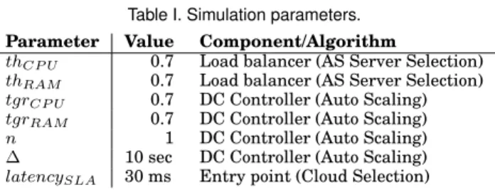
Ire-Table I. Simulation parameters.
Parameter Value Component/Algorithm
thCP U 0.7 Load balancer (AS Server Selection)
thRAM 0.7 Load balancer (AS Server Selection)
tgrCP U 0.7 DC Controller (Auto Scaling)
tgrRAM 0.7 DC Controller (Auto Scaling)
n 1 DC Controller (Auto Scaling)
∆ 10 sec DC Controller (Auto Scaling)
latencySLA 30 ms Entry point (Cloud Selection)
land and the other one in New York, US. These are actual locations of EC2 availability zones. Later on we call these data centres DC-EU-E and DC-US-E respectively. We assign the VMs from these data centres IP address from Dublin and New York respec-tively, which are extracted from GeoLite. All VMs we allocate in these data centres have the performance characteristics and the price of EC2 m1.small instances with Linux in the respective AWS regions. We model the VM start-up times based on the empirical performance study by Mao and Humphrey [2012]. Just like in Amazon EC2, the on-demand VM billing inDC-EU-EandDC-US-Eis done per hour.
To demonstrate the usage of heterogeneous cloud resources from multiple cloud providers, we model the other two data centres after Google Compute Engine. We po-sition them in Hamina, Finland and Dalles, US as these are actual locations of Google data centres and we assign all their VMs IP addresses from these locations. We call these data centresDC-EU-GandDC-US-G. All VM characteristics and prices are mod-elled after the n1-standard-1-dVM type in the respective locations. As Google Com-pute Engine is a new cloud offering, there is no statistical analysis of its VM booting times. Thus in our simulation we consider the start-up time of an1-standard-1-dVM to be the same as the one of an EC2 m1.smallVM. Like in Google Compute Engine, VMs in DC-EU-G and DC-US-Gare billed in 1 minute increments and all VMs are charged for 10 minutes at least.
In our simulation we deploy the aforementioned 3-tier architecture and brokering components, as described in the previous sections. We model one entry point VM in each data centre. To demonstrate how our approach handles resource contention in the data layer, in the experiments we assume that in each cloud the DB layer is static (i.e. not scalable) and consists of 2 DB servers, holding equal in size database shards. Table I summarises the values of the algorithms’ parameters that we use in the simu-lation.
6.2. Experimental Application and Workload
We base our experimental workload on the Rice University Bidding System (RUBiS) benchmarking environment [RUBiS 2014], [Amza et al. 2002]. RUBiS implements an e-commerce dynamic web site similar to eBay.com and follows the 3-tier architectural pattern having AS and DB servers.
RUBiS’s main and to the best of our knowledge newest competitor in the area of 3-tier application benchmarking is CloudSuite’s CloudStone [2014]. Unlike RUBiS, which has a simple synchronous web interface lacking any JavaScript, CloudStone im-plements more sophisticated asynchronous (i.e. AJAX) web user interface. While this is important for evaluating how end-users interact with a system, in this work we are interested in how to provision for and load balance the incoming server side requests. RUBiS follows the guidelines of the TPC-W [2002] specification of the Transaction Processing Performance Council (TPC), which is an industry standard for testing 3-tier e-commerce systems. The RUBiS client implements features like end user “think times” and page transitions in accordance with the predefined statistical distributions defined in TPC-W. That is why it is our method of choice for a typical 3-tier application
Time after experiment's start
A
v
er
age Session Arr
iv als 0h 3h 6h 9h 12h 15h 18h 21h 24h 0 2000 4000 6000 8000 EU US
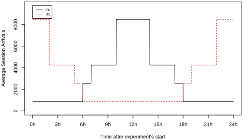
Fig. 3. User arrival frequencies per minute in the entry points of the EU data centres (DC-EU-E,DC-EU-G)
and the US ones (DC-US-E,DC-US-G).
in terms of incoming server requests patterns per user compared to CloudStone, which does not follow a public specification.
The RUBiS workload consists of sessions, each of which consists of a string of user requests. We have deployed in a local virtualised environment the PHP version of RUBiS with a standard non-clustered MySql database in the backend and we run a test with 100 concurrent sessions. During the test we monitor how the performance utilisations (in terms of CPU, RAM and disk) of the servers change over time as a result of the executed workload. Based on that, we define the performance utilisations over time of a typical RUBiS session. We will not describe the exact procedure for extracting a session performance model, as our previous work [Grozev and Buyya 2013] details this procedure and demonstrates experimentally the validity of the extracted model. We use this derived session performance model for our simulation.
The number of incoming sessions over a short time period can be well modelled with Poisson distribution with a constant meanλ[Cao et al. 2003], [Robertson et al. 2003]. However, over larger time periods the frequencies of user arrivals can change and are rarely constant. Hence, the number of session arrivals over time can be represented as a Poisson distribution over a frequency function of timeλ(t), which represents the variations in session arrival frequencies [Grozev and Buyya 2013].
Our experiment has a duration of 24 hours with workload which is more intensive during working hours and lower otherwise. We model the user arrival frequencies in the entry points of the two European (EU) data centres to be the same. The arrival frequencies in the US data centres are the same as those in the EU ones, only “shifted” with 12 hours to represent the time zone difference. Figure 3 depicts how the arrival frequencies per minute (i.e.λ(t)) in the entry points of the European and the US data centres change over time.
In our simulation, each user/session is assigned an IP address, which as explained previously can be used to approximate the user’s physical location and the latencies to the candidate data centres. The GeoLite [2014] database provides IP ranges for every country. In the simulation, whenever we model the arrival of a user in a US data centre, we take a random US IP from GeoLite. Similarly, all users arriving in the EU data centres are assigned random IP addresses from EU countries.
To demonstrate how our system handles regulatory requirements, we introduce an additional legislative constraint. In the simulation we assign a citizenship to each user and impose the requirement that a user with US citizenship should be served
in a US data centre and a EU citizen should be served in the EU. As discussed we implement this logic in the admission controllers. We assign US citizenship to 10% of the users arriving in the EU entry points, and EU citizenship to 10% of the users arriving in the US clouds. Furthermore in our simulation the data of all EU citizens is replicated in both EU data centres, and the data of all US citizens is replicated in both US cloud sites. Therefore, a EU or US citizen can be served in any EU or US data centre respectively.
6.3. Baseline Approach
We compare our approach to a baseline method which uses the standard industry prac-tices. More specifically, we have implemented a baseline simulation, which distributes the incoming users to the data centres that can serve them with the lowest latency, similarly to the Route 53 LBR service [Amazon 2014c]. Following the design of the AWS Elastic Load Balancer [Amazon 2014d], within each data centre we implement sticky load balancing that assigns new sessions to running AS servers following the Round-robin algorithm. Lastly, in our baseline simulation we implement automatic autoscaling following the design of AWS AustoSale [Amazon 2014a]. More specifically, if all AS servers within a data centre reach CPU utilisation of more than 80% – a new AS server is started. If an AS server reaches CPU utilisation below 10% it is stopped. We have also implemented acool downperiod of 2.5 minutes. Just like in AWS AustoS-ale, we do not allow for two consequent autoscaling actions to happen within a period shorter than thecool downperiod.
6.4. Results
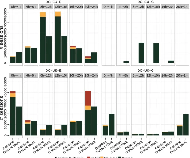
Figure 4 depicts the number of served sessions in each data centre over time. On the diagram a session is classified asfailed if some of the servers handling it failed (e.g. due to out of memory error). A session isrejectedif it is assigned to a data centre which is not eligible to serve it. In our simulation, this happens if a US citizen is assigned to a European data centre or vice versa. Otherwise, a session is consideredserved.
From Figure 4 we can see that the baseline approach redirects much fewer sessions to data centresDC-EU-GandDC-US-Gin comparison to the others. This is because of the location of these data centres and the end users. As described, in our experiment all IP addresses within EU and US are likely to be used as sources of sessions with the same probability. As to the GeoLite database, and the PingER service, there are much more IP addresses located nearby and with lower latency to Dublin, Ireland and New York, US than to Hamina, Finland and Dalles, Oregon, US. Therefore, the baseline approach redirects the majority of incoming sessions to these data centres. As the data layer cannot scale up, this leads to resource contention during peak workload periods (10h-14h in the EU data centres and 22h-24h, 0h-2h in the US). This in turns causes congestion in the DB servers resulting in slowdown in session serving. As a result the number of concurrently served sessions is increased significantly, causing AS servers keeping in memory the sessions’ states to fail with “out of memory” errors (in the case ofDC-US-E) or to degrade response time (in the case ofDC-EU-E).
Another reason for session failure in the baseline approach is the autoscaling, which terminates AS servers with low utilisation even if they serve sessions. This is visible in the case ofDC-EU-Eduring the 16h-24h period and inDC-US-Eduring the 0h-4h period, when the scaling down causes several session failures, as sessions are stateful. Our approach terminates servers only if they do not serve any sessions, and thus re-duces the number of session failures for stateful applications. Consequently the overall rate of session failures in the baseline is approximately 7%.
In contrast to the baseline approach, during the workload peak periods our approach redirects many sessions toDC-EU-GandDC-US-G, even though they may not be
opti-0h−4h 4h−8h 8h−12h 12h−16h 16h−20h 20h−24h 0 10000 20000 30000 40000 50000
# sessions
DC−EU−E 0h−4h 4h−8h 8h−12h 12h−16h 16h−20h 20h−24h DC−EU−G 0h−4h 4h−8h 8h−12h 12h−16h 16h−20h 20h−24h 0 10000 20000 30000 40000 50000 Baseline Current W ork Baseline Current W ork Baseline Current W ork Baseline Current W ork Baseline Current W ork Baseline Current W ork# sessions
DC−US−E 0h−4h 4h−8h 8h−12h 12h−16h 16h−20h 20h−24h Baseline Current W ork Baseline Current W ork Baseline Current W ork Baseline Current W ork Baseline Current W ork Baseline Current W ork DC−US−GSession Outcome: Failed Rejected Served
Fig. 4. Session outcome over time.
mal in terms of cost or latency. This is because the cost of a data centre is evaluated as
+∞if it is overloaded (see Eq. 2) and this is used by the cloud selection Algorithm 3. As a result, our approach minimises session failure by diverting users from overloaded data centres to alternative ones. During off-peak hours, our approach also redirects most users toDC-EU-E andDC-US-E, which as discussed is optimal in terms of la-tency.
Furthermore, the baseline approach does not consider the stated regulatory require-ments during the cloud selection stage and only uses the latency as selection criteria. Thus about 10% of the incoming sessions are redirected to ineligible clouds and are rejected. In contrast, our approach takes this into consideration, and redirects users to eligible data centres, even if this means sub-optimality in terms of latency and cost.
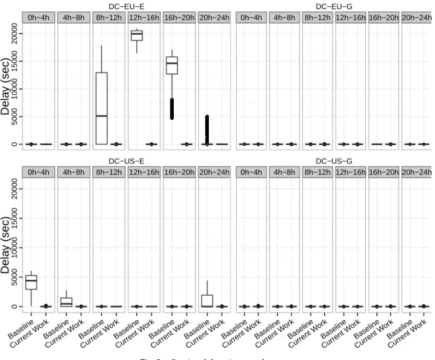
A session delay is defined as the sum of the latency delay and the execution delay. The latency delay is the time lost in network transfer between a user and the cloud during a session. Execution delay is the time lost due to resource contention (e.g. CPU preemtion) on the server side. The session delay is a measurement of the end user experience. The simulation environment allows us to measure execution delay [Grozev