MATHEMATICAL ENGINEERING
TECHNICAL REPORTS
An Iterated Local Search Algorithm
for the Vehicle Routing Problem
with Convex Time Penalty Functions
Toshihide Ibaraki, Shinji Imahori, Koji Nonobe,
Kensuke Sobue, Takeaki Uno, Mutsunori Yagiura
METR 2006–36 June 2006
DEPARTMENT OF MATHEMATICAL INFORMATICS
GRADUATE SCHOOL OF INFORMATION SCIENCE AND TECHNOLOGY THE UNIVERSITY OF TOKYO
BUNKYO-KU, TOKYO 113-8656, JAPAN
The METR technical reports are published as a means to ensure timely dissemination of scholarly and technical work on a non-commercial basis. Copyright and all rights therein are maintained by the authors or by other copyright holders, notwithstanding that they have offered their works here electronically. It is understood that all persons copying this information will adhere to the terms and constraints invoked by each author’s copyright. These works may not be reposted without the explicit permission of the copyright holder.
An Iterated Local Search Algorithm for the Vehicle Routing
Problem with Convex Time Penalty Functions
Toshihide Ibaraki 1 Shinji Imahori 2 Koji Nonobe 3
Kensuke Sobue 4 Takeaki Uno 5 Mutsunori Yagiura 6
1 Department of Informatics, School of Science and Technology, Kwansei Gakuin University, Sanda 669-1337, Japan.
E-mail: [email protected]
2 Department of Mathematical Informatics, Graduate School of Information Science and Technology, University of Tokyo, Tokyo 113-8656, Japan.
E-mail: [email protected]
3 Department of Art and Technology, Faculty of Engineering, Hosei University, Koganei 184-8584, Japan.
E-mail: [email protected]
4 Toyota Motor Corporation, Toyota 471-8571, Japan. 5 National Institute of Informatics, Tokyo 101-8430, Japan.
E-mail: [email protected]
6 Department of Computer Science and Mathematical Informatics,
Graduate School of Information Science, Nagoya University, Nagoya 464-8603, Japan. E-mail: [email protected]
Abstract: We propose an iterated local search algorithm for the vehicle routing problem with time window constraints. We treat the time window constraint for each customer as a penalty function, and assume that it is convex and piecewise linear. Given an order of customers each vehicle to visit, dynamic programming (DP) is used to determine the optimal start time to serve the customers so that the total time penalty is minimized. This DP algorithm is then incorporated in the iterated local search algorithm to efficiently evaluate solutions in various neighborhoods. The amortized time complexity of evaluating a solution in the neighborhoods is a logarithmic order of the input size (i.e., the total number of linear pieces that define the penalty functions). Computational comparisons on benchmark instances with up to 1000 customers show that the proposed method is quite effective, especially for large instances.
Keywords: Vehicle routing problem with time windows, metaheuristics, dynamic programming
1
Introduction
The vehicle routing problem(VRP) is the problem of minimizing the total distance traveled by a number of vehicles, under various constraints, where each customer must be visited exactly once by a vehicle. This is one of the representative combinatorial optimization problems and is known to be NP-hard. Among variants of VRP, the VRP with capacity and time window constraints, called the vehicle routing problem with time windows (VRPTW), has been widely studied in the last decade. The capacity constraint signifies that the total load on a route cannot
1 INTRODUCTION 2
exceed the capacity of the vehicle serving the route. The time window constraint signifies that each vehicle must start the service at each customer in the period specified by the customer. The VRPTW has a wide range of applications such as bank deliveries, postal deliveries, school bus routing and so on. For an extensive survey on heuristic and metaheuristic approaches for the VRPTW, see references [5, 6] by Br¨aysy and Gendreau.
If the capacity and time window constraints must be satisfied strictly, such problem is called the VRPHTW (H stands for hard). For this problem, even just finding a feasible solution with a given number of vehicles is known to be NP-complete, because it includes the (one-dimensional) bin packing problem [10] as a special case. Thus, it is inefficient to search only within the feasible region of the VRPHTW, especially when the constraints are tight. Moreover, in many real-world situations, these constraints can be violated to some extent. Considering these, we treat these two types of constraints as soft (i.e., can be violated) in this paper. This problem is called the VRPSTW (S stands for soft), and the amount of violation of soft constraints is penalized by using penalty functions and added to the objective function. In this case, it is not trivial to determine the optimal start time of services at all customers so that the total penalty is minimized after fixing the order of customers for each vehicle to visit.
The time penalty function is the function that penalizes the amount of violation of time window constraints for customers. In most of the previous work for the VRPTW [23, 28, 29, 31], only one time window is allowed for each customer and in this case the time penalty function is convex. In the literature [8, 11, 23, 31], algorithms for particular convex time penalty functions were proposed in order to treat the time window constraint as a soft constraint. In [31], the time penalty for each customer is +∞ for earliness and linear for tardiness, and an O(1) time algorithm to compute approximately the optimal time penalty for a solution in neighborhoods was proposed. In [8, 23], the time penalty is linear for both of earliness and tardiness, and
O(n2k) time algorithms to compute the penalty of a given route of vehicle k were proposed, wherenkis the number of customers assigned to vehiclek. If the time penalty function for each
customer is the absolute deviation from a specified time, the problem to determine the optimal start time of services at all customers is called the isotonic median regression problem, which has been extensively studied. To our knowledge, the best time complexity for this problem (for a vehiclek) is O(nklognk) [1, 11, 17].
The problem with multiple time windows [9, 20] and other variants of VRPTW [16, 30] have also been considered. In our previous paper [20], the time penalty function can be non-convex and discontinuous as long as piecewise linear. Letδk be the total number of linear pieces of the
time penalty functions for the depot and all customers assigned to vehiclek, and letδmaxbe the
maximum of δk among all vehicles. We proposed a dynamic programming (DP) algorithm that
runs in O(nkδk) time when the problem of minimizing the time penalty of vehicle k is solved
from scratch. This DP algorithm was incorporated into metaheuristic algorithms based on local search. We also designed a sophisticated data structure with which the optimal time penalty of a solution in neighborhoods is computed inO(δmax) amortized time. However, this computation
time is still expensive when the number of customers becomes large, since δk usually depends
linearly on the number of customers assigned to vehicle k. Moreover, it is observed in many practical situations that each customer has only one time window. In this paper, hence, the time penalty function is assumed to be convex and piecewise linear.
One of the main contribution of this paper is to propose an efficient algorithm to deal with convex time penalty functions. We use the DP technique in order to compute the optimal time penalty of a vehicle that serves customers in a specified order. The time complexity of our DP algorithm for convex time penalty functions isO(δklogδk) for each vehicle k, while the time to
2 PROBLEM 3
The essential part of the VRP, i.e., assigning customers to vehicles and determining the visiting order of each vehicle, is determined by a local search (LS) algorithm. We use basic neighborhoods such as the cross exchange and 2-opt∗, limiting the neighborhood sizes by using parameters. The LS based on these neighborhoods is then incorporated in the framework of metaheuristics. Among many possible metaheuristics based on the LS, we utilize the iterated local search (ILS) [21]. As it is not easy to specify appropriate weights of constraints a priori, we introduce a mechanism of adaptively controlling penalty weights into the ILS, which turns out to be very effective.
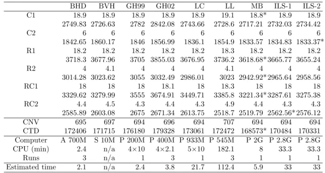
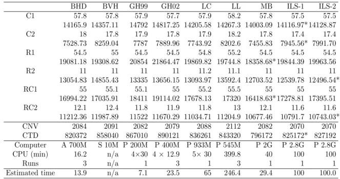
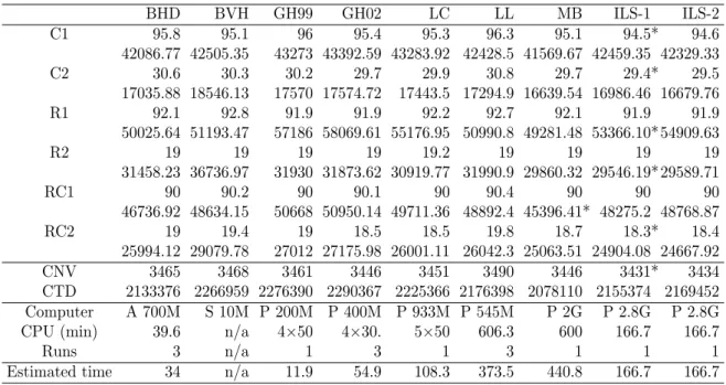
To see the performance of our algorithm, we conduct computational experiments on rep-resentative benchmark instances of the VRPTW: (1) Solomon’s benchmark instances [29] and (2) Gehring and Homberger’s benchmark instances [13]. For Solomon’s instances, the solu-tion quality of our algorithm is competitive with those of recent algorithms developed for the VRPTW. For Gehring and Homberger’s instances, our results are the best among the tested algorithms. This tendency becomes clearer for larger scale instances such as ones with 800 or 1000 customers. It should be pointed out that these benchmark instances are special cases of the instances that our algorithm can treat.
The remainder of this paper is organized as follows. In Section 2, we define the problem that we consider in this paper. In Section 3, we explain the problem to determine the optimal start time of services for a given route, and propose a DP algorithm. In Section 4, we propose local search and metaheuristic algorithms for finding a good set of routes. In Section 5, we propose some ideas to accelerate the speed of our local search algorithm. In Section 6, we show our computational results on representative benchmark instances with up to 1000 customers. We give concluding remarks and discuss some extensions of our algorithm in Section 7.
2
Problem
In this section, we formulate the vehicle routing problem with convex time penalty functions. LetG= (V, E) be a complete directed graph with a vertex setV ={0,1, . . . , n}and an edge set
E ={(i, j) |i, j ∈V, i6=j}, and M ={1,2, . . . , m} be a set of vehicles. Vertex 0 is the depot and other vertices are customers. The following parameters are associated with each customer
i∈V \ {0}, the depot, each edge (i, j)∈E, and each vehiclek∈M:
• an amountqi (≥0) of the resource to be delivered from the depot to customeri,
• a service timeui (≥0) at customeri,
• a time penalty function pi(t) (≥0) of the start timetof the service for customer i,
• a time penalty function pd
0(t) (≥0) of the departure time tfrom the depot,
• a time penalty function pa0(t) (≥0) of the arrival timet at the depot,
• a distancedij (≥0) for edge (i, j),
• a travel time tij (≥0) for edge (i, j),
• a capacityQk (≥0) for vehiclek.
Distances dij and travel times tij are asymmetric in general; i.e., dij =6 dji and tij 6= tji may
2 PROBLEM 4
For convenience, we assume mintpi(t) = 0, mintp0d(t) = 0 and mintpa0(t) = 0 without loss of
generality. It is also assumed that each function is represented by a linked list of linear pieces. We define a routeby a sequence of the customers served by one vehicle. Let σk denote the
route traveled by vehicle k, and σ = (σ1, σ2, . . . , σm). We denote by σk(h) the hth customer
in σk, and we defineσk(0) = σk(nk+ 1) = 0, where nk is the number of customers for vehicle
k ∈ M (i.e., each vehicle k starts from the depot, visits nk customers, and comes back to the
depot). We define 0-1 variablesyik(σ)∈ {0,1}fori∈V \ {0} andk∈M by
yik(σ) = 1 ⇐⇒ ∃h∈ {1,2, . . . , nk}, i=σk(h).
That is,yik(σ) = 1 if and only if vehiclekvisits customeri. Moreover, letsi be the start time of
service at customeri,sdkbe the departure time of vehicle kfrom the depot and sak be the arrival time of vehicle k at the depot, and let s = (s1, s2, . . . , sn, sd1, sd2, . . . , sdm, sa1, sa2, . . . , sam). Note
that each vehicle is allowed to wait at customers before starting services. The total traveling costdsum(σ) of all vehicles, the total penaltypsum(s) for time window constraints, and the total
amount qsum(σ) of capacity excess are expressed as
dsum(σ) = X k∈M nk X h=0 dσk(h)σk(h+1), psum(s) = X i∈V\{0} pi(si) + X k∈M pd 0(sdk) + X k∈M pa 0(sak), qsum(σ) = X k∈M max X i∈V\{0} qiyik(σ)−Qk, 0 .
The vehicle routing problem with convex time penalty functions is now formulated as follows:
minimize cost(σ,s) =dsum(σ) +psum(s) +qsum(σ) (1)
subject to X k∈M yik(σ) = 1, i∈V \ {0}, (2) sdk+tσk(0)σk(1) ≤sσk(1), k∈M, (3) sσk(h)+uσk(h)+tσk(h)σk(h+1) ≤sσk(h+1), k∈M, h= 1,2, . . . , nk−1, (4) sσk(nk)+uσk(nk)+tσk(nk)σk(nk+1) ≤sak, k∈M. (5)
Constraint (2) means that every customeri∈V \ {0}must be served exactly once by a vehicle. Constraints (3) and (4) require that the start timesiof service for customerimust not be before
the arrival time at customer i, and constraint (5) means that each vehicle k can return to the depot only after serving all the customers assigned to vehiclek. As for the objective function (1), the time window and capacity constraints are treated as soft constraints, and their violations are evaluated as the penaltiespsum(s) andqsum(σ), respectively, in the objective function. Note that
the weighted sumdsum(σ) +µppsum(s) +µqqsum(σ) with constantsµp (≥0) andµq(≥0) might
seem more general; however, such a weighted sum can be represented in the above formulation by regarding µppi(t), µppd0(t),µppa0(t), µqqi and µqQk (i∈V \ {0},k∈M) as the given input,
and hence the weights are omitted for simplicity unless otherwise stated.
Note that we call a solution that satisfies constraints (2) to (5) a feasible solution throughout the paper; i.e., a feasible solution does not necessarily satisfy the time window and capacity constraints. If time window and/or capacity constraints are to be satisfied, the penaltiespsum(s)
3 OPTIMAL START TIME OF SERVICES 5
Remark: Although the numbermof vehicles is sometimes treated as a decision variable in the literature, we consider it as a given constant in this paper for the following two reasons. (1) In many applications, the number of vehicles m is fixed. (2) Algorithms become simpler if m is treated as a constant, since route elimination operators will not be necessary. For problems wheremis a decision variable, we need to try various values ofmto find a small feasiblem; however, in many practical situations, an appropriate range ofmis known in advance.
3
Optimal start time of services
In this section, we consider the problem of determining the start time to serve the customers in a given route σk so that the total time penalty is minimized. This problem can be solved
independently for each route. (How to determine a routeσkwill be discussed in Section 4.) We
call this problem the optimal start time problem, which is described as follows: minimize pd0(sdk) + nk X i=1 pσk(i)(sσk(i)) +p a 0(s a k), subject to sdk+tσk(0)σk(1) ≤sσk(1), sσk(h)+uσk(h)+tσk(h)σk(h+1)≤sσk(h+1), h= 1,2, . . . , nk−1, sσk(nk)+uσk(nk)+tσk(nk)σk(nk+1)≤sak.
Letδ(p) be the number of pieces in a piecewise linear functionp(t), and let the total number of pieces in the penalty functions for all customers in a route σk (including the depot) be
δk =
Pnk
h=1δ(pσk(h)) +δ(pd0) +δ(pa0). We propose an O(δklogδk) time algorithm to solve this
problem by dynamic programming (DP). For this problem, there are several efficient algorithms that have the same time complexity as the algorithm in this section [1, 17]. However, our DP algorithm is simpler and utilized to design a more efficient algorithm for evaluating solutions in various neighborhoods in Section 5.1.2.
3.1 Dynamic programming
We define functions fk
h(t) for h= 0,1, . . . , nk+ 1 to be the minimum sum of the penalty values
for customersσk(0), σk(1), . . . , σk(h) under the condition that all of them are served in this order
and the service for σk(h) starts by time t. We call this theforward minimum penalty function.
For convenience, we also define values
τhk =uσk(h)+tσk(h)σk(h+1)
for customersh= 1,2, . . . , nk; i.e.,τhkis the sum of the service time at thehth customer and the
travel time from this to the next customer. Based on the idea of DP,fhk(t) can be computed by
f0k(t) = min t0≤t p d 0(t0), fhk(t) = min t0≤t ³ fhk−1(t0−τhk−1) +pσk(h)(t0) ´ , h= 1,2, . . . , nk, fnkk+1(t) = min t0≤t ³ fnk k(t 0−τk nk) +p a 0(t0) ´ , (6)
where τ0k = tσk(0)σk(1). The minimum time penalty value for the entire route σk (denoted by
p∗sum(σk)) can be obtained by
p∗sum(σk) = min t f
k
3 OPTIMAL START TIME OF SERVICES 6
Moreover, the optimal start timesσk(h) of the service for each customerσk(1), σk(2), . . . , σk(nk),
the departure time sdk from the depot and the arrival time sak at the depot can be computed backward by sak = arg min t f k nk+1(t), sσk(h) = arg min t≤sσk(h+ 1)−τ k h fhk(t), h=nk, nk−1, . . . ,1, sdk = arg min t≤sσk(1)−τ k 0 f0k(t), (8) wheresσk(nk+1)=sak.
3.2 Algorithm and time complexity
In this section, we consider the data structure and algorithm for computing forward minimum penalty functionsfhk in the recurrence formula (6).
We first consider some characteristics of fhk. Since functions pi, pd0 and pa0 are convex and
piecewise linear, eachfhkis also convex and piecewise linear. Moreover, eachfhkis nonincreasing by definition. The number of linear pieces for fhk is O(δk).
In order to computefhkin the recurrence formula (6), we need the following three operations: 1. Computingf(t) :=f(t−τ) (called shift operation).
2. Computingf(t) :=f(t) +g(t) (called add operation). 3. Computingf(t) := mint0≤tf(t0) (called minimize operation).
Recall that functions f and g are convex and piecewise linear, and τ is a constant. Note also that we represent function g by a linked list of linear pieces. To support the above operations efficiently, we use the following data structure to represent function f:
• A balanced binary search tree withδ(f) leaves, whose height is denoted byhtreeand has a valuec (called tree value). Each leaf v has an interval [tlv, trv], and each node v(including internal nodes and leaves) of this tree has values av,bv andζv.
• Each leaf of the tree represents a linear piece of function f, where the αth leaf in the inorder corresponds to theαth linear piece off counted from left.
We denote the root of the tree byv0, and the parent, the left child and the right child of a nodev
by H(v), L(v) andR(v), respectively. We also denote the rightmost leaf in the descendants of an internal nodev by ˜R(v), and we define ˜R(v) =vfor each leafv. Each nodev has pointers to
H(v),L(v),R(v) and ˜R(v), if they exist. We represent the set of nodes in the path from a nodev
to a nodev0 as℘(v, v0), wherev0 is a descendant of v. Consider a linear piece of functionf that has a gradienta, an interceptb and an interval [tl, tr], which is assigned to leafv. The interval
of leaf v satisfies [tl
v, trv] = [tl−c, tr−c], wherec is the tree value. The valuesav0 and bv0 kept
in nodesv0∈℘(v0, v) satisfy the following equations:
X v0∈℘(v0,v) av0 =a, X v0∈℘(v0,v) bv0 =b.
The tree value c, intervals [tlv, trv] of leaves v, and values av and bv of nodes v are appropriately
3 OPTIMAL START TIME OF SERVICES 7
It is possible to shift a function f inO(1) time by updating the tree value c. For a givent, we can find the linear piece whose interval [tl, tr] satisfiestl ≤t < tr in O(htree) time: We first
set v := v0. For the leaf node ˜R(L(v)), if t < trv+c holds, then we set v := L(v). Otherwise,
we set v := R(v). We repeat this operation until v becomes a leaf node of the tree, and then output the linear piece corresponding to the leafv.
As for the value ζv of each nodev, we set
ζv =
X
v0∈℘(v,R˜(v)) av0.
It is also possible to find the rightmost linear piece whose gradient is less than a given constant
α in O(htree) time: We first setv := v0. The gradient of the linear piece corresponding to the
leaf node ˜R(L(v)) can be computed by
X
v0∈℘(v0,v)
av0+ζL(v). (9)
If it is larger than or equal toα, we setv:=L(v). Otherwise, we setv:=R(v). We repeat this operation until v becomes a leaf, and output the linear piece corresponding to the leaf v. The computation of (9) can be done in constant time for each v, because we can use the value of
P
v0∈℘(v0,H(v))av0 already computed for the parent.
We now explain how to calculate and store the function fhk by using this data structure. First, we show the procedure for the first equation of (6). We construct a balanced binary tree with leaves corresponding to the linear pieces of pd0 whose gradients are less than 0. For each leaf v, we set an interval [tlv, trv] and values av, bv for the corresponding linear piece. We add
another leaf v to the rightmost position of this tree; av is 0, trv is +∞, and we setbv and tlv so
that the resulting function becomes continuous. We set c = 0 for this tree, av = 0 andbv = 0
for all internal nodesv, andζv =aR˜(v)for all nodesv. The time complexity of this computation
isO(δ(pd0)).
We then explain the procedure for the second equation of (6). Since the procedure for the third equation is similar, we omit its explanation. For the shift operationfhk−1(t0−τ), we update the tree value by c := c+τ so that the intervals of the leaves are shifted. The add operation
fhk−1(t0−τ) +pσk(h)(t0) is realized as follows. Our basic strategy for this operation is adding each linear piece of g(t) (=pσk(h)(t0)) to function f(t) (=fhk−1(t0−τ)) one by one. Consider a situation of adding a linear piece having gradienta, interceptband interval [tl, tr] to the binary
tree corresponding to the functionf(t) with tree valuec. We find the leafvα(resp.,vβ) satisfying
tlvα ≤tl−c < trvα (resp.,t l vβ < tr−c ≤t r vβ). Ift l
vα 6=tl−cholds, we divide leafvα into two leaves
which have intervals [tlvα, tl−c] and [tl−c, trvα], and call the new leaf with interval [tl−c, t r vα]
asvα. We divide leaf vβ into two leaves and definevβ similarly (if necessary). In order to add
the gradientaand interceptbto leaves whose intervals are [tl−c, trvα],[t r
vα, t00], . . . ,[t l
vβ, tr−c], we
addaandbto the values av and bv of nodesvthat satisfy one of the following three conditions:
1. R(H(v)) =v,H(v) is not an ancestor ofvβ but that ofvα,v is not an ancestor ofvα,
2. L(H(v)) =v,H(v) is not an ancestor of vα but that ofvβ,v is not an ancestor of vβ,
3. v=vα orv=vβ.
It is easy to see that the number of nodes whose values are changed is O(htree) and we can change those values in O(htree) time. The resulting tree may not satisfy the conditions of a
4 LOCAL SEARCH FOR FINDING A GOOD SET OF ROUTES 8
balanced tree; we apply a balancing procedure that runs in O(htree) time if necessary. Such an insertion is conducted for all linear pieces of g(t). Thus, the time complexity of computing
f(t) +g(t) isO(δ(g)htree) time.
For the minimize operation mint0≤t
¡
fhk−1(t0−τ) +pσk(h)(t0)
¢
, we find the rightmost linear piece whose gradient is less than 0 in O(htree) time. Recall that functionfhk−1(t−τ) +pσk(h)(t)
is convex. We then remove the unnecessary portion of the tree (i.e., those with nonnegative gradient), and add a new leafv to the rightmost position of this tree; av is 0,trv is +∞, and we
setbvandtlv so that the resulting function becomes continuous. We apply a balancing procedure
for this tree (if necessary). The computational complexity for these operations isO(htree). Now, we estimate the time complexity of our DP algorithm. We can compute fk
nk+1 in
O(δklogδk) time using the above procedures and operations, since htree = O(logδk) holds
throughout the algorithm.
For the computation of (8) and algorithms in Section 5, we must store fk
h for all h =
0,1, . . . , nk+ 1. If we realize this naively, just by keeping the binary search trees of all functions
independently, we needO(nkδk) time and space. To avoid this, we share common parts among
the trees to save the computation time and memory. Consider the case of computing fk h. We
first generate a tree with only the root node v0 and set L(v0) = L(v00), R(v0) = R(v00) and
˜
R(v0) = ˜R(v00), wherev00is the root offhk−1. Then, whenever we need to update some information
of a node in the process of computing fhk, we duplicate the node and apply the updates only on the copy, while sharing the other nodes with the tree of fk
h−1. As the number of new
nodes is proportional to the number of updates, we can calculate and store functions fhk for all
h= 0,1, . . . , nk+ 1 inO(δklogδk) time and space.
After computing the functionsfhkby (6), we can compute the minimum time penalty value for routeσk inO(logδk) time by (7), and the optimal start timesσk(h) of services for all customers
in this route in O(nklogδk) time by (8).
4
Local search for finding a good set of routes
In this section, we describe a local search (LS) algorithm to find a good set of routes. The following ingredients must be specified in designing the LS: Search space, how to generate an initial solution, a function to evaluate solutions, neighborhoods and move strategy. The search space of our LS is the set of all visiting orders σ = (σ1, σ2, . . . , σm) satisfying condition (2).
Note that a set of visiting orders σ is called a “solution” in Sections 4 and 5, while a solution means (σ,s) in other parts of this paper. We generate an initial solution (i.e., an initial set of visiting orders) randomly. The objective function is often used in the literature as the evaluation function; however, we do not use the objective function directly in this paper. The details of our evaluation function will be explained in Section 4.1. The neighborhoodN(σ) of a feasible solution σ is a set of solutions obtainable from σ by applying some specified operations. In Section 4.2, we explain the neighborhoods utilized in our LS. As the move strategy, we adopt (a slightly simplified version of) the aspiration plus strategy [14], which will be explained in Section 5.1. We describe a metaheuristic algorithm based on the LS in Section 4.3.
4.1 Evaluation function
Letp∗sum(σ) be the minimum value ofpsum(s) among thosessatisfying conditions (3) to (5) for
a given set of routesσ. Such an scan be computed by solving the optimal start time problem for each route with the DP algorithm of Section 3. (A more efficient method will be presented in Section 5.1.2.)
4 LOCAL SEARCH FOR FINDING A GOOD SET OF ROUTES 9
Then the objective function (1) becomes
cost(σ) =dsum(σ) +psum∗ (σ) +qsum(σ). (10)
Using this objective function as an evaluation function of LS may not work well for problem instances with hard time window and/or capacity constraints. In such cases, a large amount of penalty should be imposed on the violation of the time window and/or capacity constraints to satisfy them strictly, but it prevents the search from visiting the infeasible region of VRPHTW. To avoid such phenomenon, we therefore adopt the following functioneval(σ) instead ofcost(σ) to evaluate solutions in LS:
eval(σ) =dsum(σ) +κppsum∗ (σ) +κqqsum(σ), (11)
whereκp (resp.,κq) is a weight of psum∗ (σ) (resp., qsum(σ)). We change these weights whenever
a local search stops at a locally optimal solution. As for the control mechanism of parametersκp
and κq in our evaluation function eval, we control them as follows. If we find a solution whose time penalty (resp., capacity penalty) is equal to 0 in LS, the time penalty weight κp (resp.,
the capacity penalty weight κq) is decreased to 0.9κp (resp., 0.9κq) after completion of LS in order to emphasize the other partdsum(σ) +qsum(σ) (resp., dsum(σ) +p∗sum(σ)). Otherwise,κp
(resp., κq) is increased to min{1.1κp,1} (resp., min{1.1κq,1}) after completion of LS so that
the influence ofp∗sum(σ) (resp.,qsum(σ)) is reduced.
4.2 Neighborhoods
The neighborhood is a very important factor that determines the effectiveness of LS. In our algorithm, we utilize some standard neighborhoods for the VRP such as the cross exchange and 2-opt∗ neighborhoods, limiting their sizes by using parameters.
Iopt neighborhood The iopt neighborhood [4] is a variant of Or-opt neighborhood [27] used for the traveling salesman problem (TSP), which is a special case of the VRP in which the number of vehicles is one. We define apath as a subroute; i.e., a sequence of some consecutive customers served by one vehicle. An iopt operation removes a path of length at most Lioptpath (a parameter) and inserts it into another position of the same route, where the position is limited within the lengthLioptins (a parameter) from the current position. For each insertion, we consider the following two cases: (1) visiting order preserved (called a normal insertion), and (2) visiting order reversed (called a reverse insertion). Note that the operation of just inverting the order of a path at its current position is also an iopt operation. LetNiopt(σ, k) be the set of all solutions obtainable by applying an iopt operation to routeσkof the current solutionσ= (σ1, σ2, . . . , σm),
and letNiopt(σ) =Sk∈MNiopt(σ, k). The size of the iopt neighborhood is O(nLioptpathLioptins ).
2-opt neighborhood The 2-opt neighborhood is one of the well-known neighborhoods for the
TSP. A 2-opt operation removes a path whose length is at mostL2opt(a parameter), and inserts it into its current position with the reversed order. In other words, we remove two edges from a route, and reconstruct a route with two other edges. Let N2opt(σ, k) be the set of all solutions obtainable by applying a 2-opt operation to routeσk, and letN2opt(σ) =Sk∈MN2opt(σ, k). The
size of this neighborhood isO(nL2opt). Note that ifLioptpath ≥L2opt−1, thenN2opt(σ)⊆Niopt(σ) holds. However, parameterLioptpath is usually set small in order to keep|Niopt(σ)|small, and we useN2opt(σ) with a large L2opt independently fromNiopt(σ).
5 EFFICIENT IMPLEMENTATION OF LOCAL SEARCH 10
2-opt∗ neighborhood The 2-opt∗ neighborhood, which was proposed in [28], is a variant of the 2-opt neighborhood. A 2-opt∗ operation removes two edges from two different routes (one from each) to divide each route into two parts, and exchanges the second parts of the two routes. LetN2opt∗(σ, k, k0) be the set of all solutions obtainable by applying a 2-opt∗ operation to two routes σk and σk0 of the current solution σ, and let N2opt∗(σ) = Sk6=k0N2opt
∗
(σ, k, k0). The size of the 2-opt∗ neighborhood isO(n2).
Path insertion neighborhood A path insertion operation removes a path of length at most
Lpins (a parameter) from a route σk, and insert it into a different route σk0. Let Npins(σ, k, k0)
be the set of all solutions obtainable by applying a path insertion operation to two routes σk
and σk0, and let Npins(σ) =Sk6=k0Npins(σ, k, k0). The size of the path insertion neighborhood
isO(n2Lpins). If the length of the removed path is at mostLpinsrev (a parameter), we also consider
the reverse insertion, whereLpinsrev ≤Lpins.
Cross exchange neighborhood The cross exchange neighborhood was proposed in [31]. A
cross exchange operation removes two paths from two different routes (one from each), whose length is at most Lcross (a parameter), and exchanges them. If the length of removed paths
is at most Lcrossrev (a parameter), we also consider the (both or either) reverse insertion. Let
Ncross(σ, k, k0) be the set of all solutions obtainable by applying a cross exchange operation to two routes σk andσk0, and letNcross(σ) =Sk6=k0Ncross(σ, k, k0). The size of this neighborhood
isO(n2(Lcross)2).
Combination of the neighborhoods It is often effective to combine some neighborhoods in
an LS algorithm. Our LS searches the above five types of neighborhoods in the order described as follows: iopt, 2-opt, 2-opt∗, path insertion and cross exchange. Once we find a better solution in a neighborhood, we return to the iopt neighborhood. When no improvement is achieved in the five consecutive neighborhoods, this procedure outputs a locally optimal solution for the neighborhoods and terminates.
4.3 Iterated local search
If the LS is applied only once, many solutions of better quality may remain unvisited in the search space. To overcome this, we use the iterated local search (ILS) [21], which is one of the basic frameworks of metaheuristics. In the ILS, the LS is executed iteratively and an initial solution of each LS is generated by slightly perturbing a good solution found so far. In our ILS, a random cross exchange operation, which randomly chooses two paths from two routes and exchanges them each other, is utilized to generate initial solutions. In order to generate a new initial solution, we choose r randomly from {1,2,3}, and apply random cross exchange operations r times consecutively to the incumbent solution (i.e., the best solution found by then).
5
Efficient implementation of local search
In this section, we explain various useful ideas to search the neighborhoods efficiently. In tion 5.1, we propose ideas to speed up the evaluation of solutions in neighborhoods. In Sec-tion 5.2, we show two ideas to prune the neighborhood. In SecSec-tion 5.3, we propose other ideas to accelerate the speed of our local search procedure.
5 EFFICIENT IMPLEMENTATION OF LOCAL SEARCH 11
5.1 Evaluation of solutions in neighborhoods
Let ∆dsum (resp., ∆psum and ∆qsum) be the difference in the traveling cost dsum(σ) (resp.,
the time penalty p∗sum(σ) and the capacity excessqsum(σ)) between the current solution and a
solution in its neighborhood. Then, we define ∆eval as
∆eval= ∆dsum+κp∆psum+κq∆qsum, (12)
and move to a solution whose ∆eval is negative. In the subsequent subsections, we explain how to evaluate ∆dsum, ∆psum and ∆qsum effectively, based on the following two facts: (1) A
neighborhood operation generates at most two different routes from the current solution, and (2) each new route is generated by reconnecting a constant number of paths (more precisely, at most four paths) in the current solution.
We now explain our basic strategy. At the beginning of a neighborhood search, we compute some values and functions that will be used during the neighborhood search (called prepro-cessing). We then evaluate each solution in the neighborhood quickly with those values and functions. Thus, our computation consists of the preprocessing part and the evaluation part. To avoid calling the preprocessing part too frequently, we adopt the aspiration plus strategy [14], which is explained as follows. We evaluate solutions in the neighborhood until we evaluate all the solutions in the neighborhood or we use (approximately) the same computation time that was spent for the previous preprocessing. If we can find improved solutions during the search, we move to the best solution among them. Otherwise, we continue the search for the remaining neighbors, based on the first admissible move strategy.
5.1.1 Evaluation of ∆qsum and ∆dsum
At the beginning of a neighborhood search, we compute
γ0k= 0, γhk=γhk−1+qσk(h), h= 1,2, . . . , nk, φk0 = 0, φkh=φkh−1+dσk(h−1)σk(h), h= 1,2, . . . , nk+ 1, ˆ φknk+1 = 0, ˆ φkh= ˆφkh+1+dσk(h+1)σk(h), h=nk, nk−1, . . . ,1,0,
for allk∈M. It is possible to compute all of them inO(n) time. We evaluate ∆qsumand ∆dsum
for each solution in the neighborhood using these γhk, φkh and ˆφkh.
As for ∆qsum, we observe that ∆qsum is equal to 0 for all solutions in Niopt and N2opt,
and thus we only consider solutions in N2opt∗, Npins and Ncross. The sum Phl=0hqσk(l) of the
amount of resources for thehth through the h0th customers can be computed in O(1) time by
γhk0 −γkh−1. Since there are only two different routes from the current solution and each new
route is generated by reconnecting at most three paths, the time complexity to evaluate ∆qsum
isO(1).
As for ∆dsum, the total distancePh
0−1
l=h dσk(l)σk(l+1)of thehth through theh0th customers (in
the case of the normal insertion) can be computed inO(1) time byφkh0−φkh. The total distance
Ph0−1
l=h dσk(l+1)σk(l) of the h0th through the hth customers (in the case of the reverse insertion)
can be computed inO(1) time by ˆφkh−φˆkh0. Thus, ∆dsumis also computed inO(1) time for each
5 EFFICIENT IMPLEMENTATION OF LOCAL SEARCH 12
Since the size of each neighborhood |Niopt|, |N2opt|, |N2opt∗|, |Npins| or |Ncross| is larger thanO(n) (time for preprocessing), the amortized time complexity to evaluate ∆qsumand ∆dsum
for a solution isO(1).
5.1.2 Evaluation of ∆psum
If ∆psum is computed according to (6) from scratch, it takes O(Pk∈M0δklogδk) time, where
M0 is the set of indices of the vehicles related to a neighborhood operation. (Note that
|M0| ≤ 2 holds for any neighborhood considered in this paper.) Instead of this, we propose anO(Pk∈M0logδk) =O(logδmax) time algorithm that computes ∆psumfor a solutionσ0 in the
neighborhoods, where δmax = maxk∈Mδk. We only explain the algorithm for cases where the
number of paths contained in a new route is two or three. However, this idea can be extended to a new route obtainable by reconnecting a constant number of paths (e.g., by reconnecting four paths).
In addition to the forward minimum penalty function fhk(t) of (6), we define bkh(t) as the minimum sum of the time penalty values for customers σk(h), σk(h+ 1), . . . , σk(nk), σk(nk+ 1)
under the condition that all of them are served in this order and the service forσk(h) starts at
time t or later. We call this the backward minimum penalty function. In a symmetric manner to the computation offk
h(t),bkh(t) can be computed by:
bknk+1(t) = min t0≥t p a 0(t0), bkh(t) = min t0≥t ³ pσk(h)(t0) +bkh+1(t0+τhk)´, h=nk, nk−1, . . . ,1, bk0(t) = min t0≥t ³ pd0(t0) +b1k(t0+τ0k) ´ . (13)
Each function bkh(t) is convex, piecewise linear and nondecreasing. For a vehicle k, we can calculate and store functions bkh for all h= 0,1, . . . , nk+ 1 inO(δklogδk) time.
Reconnecting two paths Let us consider the computation of the minimum time penalty on
a new route
σ0k=h0, σk1(h1)i–hσk2(h2),0i
generated by reconnecting two paths h0, σk1(h1)i and hσk2(h2),0i, where hσk(h), σk(h0)i
repre-sents the path from σk(h) to σk(h0) in route σk. Using the forward and backward minimum
penalty functions, p∗sum(σk0) can be computed by
min t ³ fk1 h1(t) +b k2 h2(t+ ˜τ(k1, k2, h1, h2)) ´ , (14) where ˜ τ¡k, k0, h, h0¢=uσk(h)+tσk(h)σk0(h0).
If we compute mint(f(t) +b(t)) for two piecewise linear convex functions f and b naively, it
takes O(δ(f) +δ(b)) time. However, using the fact that the new function f(t) +b(t) is also convex, we can compute the minimum value and the corresponding time t (denoted by s∗) in
O(logδ(f) + logδ(b)) time under the assumption that functions f and b are represented by the balanced search trees defined in Section 3.2. (If the t that achieves the minimum value of
f(t) +b(t) is not unique, we defines∗ = min arg mint(f(t) +b(t)).) We note that our procedure
5 EFFICIENT IMPLEMENTATION OF LOCAL SEARCH 13
We compute mint(f(t) +b(t)) for two convex functionsf andbby a variant of binary search
based on the following fact: Suppose that we have a linear piece off(t) that has gradientaf and
interval [lf, rf], and another linear piece of b(t) with gradient ab and interval [lb, rb]. Ifaf +ab
is less than 0, s∗ ≥ min{rf, rb} holds; otherwise, s∗ ≤ max{lf, lb} holds. For a node v in the
balanced search tree representing a functionf orb, let a(v) and [l(v), r(v)] be the gradient and interval of the linear piece that corresponds to the leaf ˜R(L(v)) (resp.,v) ifv is an internal node (resp., a leaf). We first set vf and vb to be the root nodes of the trees representing f and b,
respectively. Using the above fact, we repeat one of the following operations until both of vf
and vb become leaves: If a(vf) +a(vb) < 0 holds, then we set vf := R(vf) (i.e., vf moves to
its right child) if r(vf) < r(vb) holds, or set vb := R(vb) otherwise (i.e., r(vf) ≥ r(vb)). On
the other hand, if a(vf) +a(vb) ≥ 0 holds, then we set vf := L(vf) if l(vf) > l(vb), or set
vb :=L(vb) otherwise (i.e., l(vf)≤l(vb)). The number these operations is bounded by the sum
of the heights of the trees representing f and b, since we replace vf or vb to its child node in
each iteration. The heights of the trees are O(logδ(f)) and O(logδ(b)), respectively, and each iteration takesO(1) time. Hence the total computation time to compute mint(f(t) +b(t)) and
s∗ is O(logδ(f) + logδ(b)).
Reconnecting three paths Let us consider the computation of the minimum time penalty
of a new route
σk0 =h0, σk1(h1)i–hσk2(h2), σk2(h3)i–hσk3(h4),0i (15)
generated by reconnecting three paths. For simplicity, we consider only the case where a new route is constructed with a normal insertion. For this computation, we use the forward and backward minimum penalty functions,τhk and ˜τ(k, k0, h, h0). Moreover, for all candidates of the intermediate path (e.g.,hσk2(h2), σk2(h3)i), we compute two types of new functions ˜f
k
h,h0(t) and
˜bk
h,h0(t), and values χ(k, h, h0). The function ˜fh,hk 0(t) (resp., ˜bkh,h0(t)) is the minimum sum of the
time penalty values for customers σk(h), σk(h+ 1), . . . , σk(h0) if these customers are served in
this order and the service for customerσk(h0) (resp.,σk(h)) starts by (resp., starts on or after)
timet. Based on the idea of DP, ˜fh,hk 0(t) and ˜bkh,h0(t) can be computed by
˜ fh,hk (t) = min t0≤t pσk(h)(t 0), h= 1,2, . . . , n k, ˜ fh,hk 0(t) = min t0≤t ³ ˜ fh,hk 0−1(t0−τhk0−1) +pσk(h0)(t0) ´ , h= 1,2, . . . , nk−1, h0=h+ 1, h+ 2, . . . ,min{h+Lmax−1, nk}, (16) ˜bk h,h(t) = mint0 ≥t pσk(h)(t 0), h= 1,2, . . . , n k, ˜bk h,h0(t) = min t0≥t ³ pσk(h)(t0) + ˜bhk+1,h0(t0+τhk) ´ , h0 = 2,3, . . . , nk, h=h0−1, h0−2, . . . ,max{h0−Lmax+ 1,1}, (17)
for all k ∈ M, where Lmax = max{Lcross, Lpins}. Since pi(t), pd0(t) and pa0(t) are convex
func-tions, ˜fh,hk 0(t) (resp., ˜bkh,h0(t)) is also convex and is nonincreasing (resp., nondecreasing). We
calculate and store these functions as well as fk
h(t) and bkh(t). This computation is possible in
O(Lmaxδklogδk) time for each vehiclek. The value χ(k, h, h0) is the minimum time needed to
serve customers σk(h), σk(h+ 1), . . . , σk(h0) in this order; that is,
χ(k, h, h0) =
hX0−1
h00=h
5 EFFICIENT IMPLEMENTATION OF LOCAL SEARCH 14
Note that we can also define ˜fh,hk 0(t), ˜bh,hk 0(t) andχ(k, h, h0) for the paths of reverse direction in a
symmetric manner, and we use them to evaluate new routes constructed with reverse insertions. We now explain how to compute the minimum time penalty value of the new routeσ0kof (15). First, we consider the following two paths
h0, σk1(h1)i–hσk2(h2), σk2(h3)i
and
hσk2(h2), σk2(h3)i–hσk3(h4),0i.
For these two paths, we independently calculate the minimum time penalty values and the corresponding times s∗h
2 and s
∗
h3, which are respectively defined as follows: s∗h2 = min arg min
t ³ fk1 h1(t−τ˜(k1, k2, h1, h2)) + ˜b k2 h2,h3(t) ´ , s∗h
3 = max arg mint
³ ˜ fk2 h2,h3(t) +b k3 h4(t+ ˜τ(k2, k3, h3, h4)) ´ . (19)
Now we compute the minimum time penalty of σk0. If
s∗h3 −s∗h2 ≥χ(k2, h2, h3) (20) holds, it is given by fk1 h1 ¡ s∗h2 −τ˜(k1, k2, h1, h2) ¢ + ˜bk2 h2,h3 ¡ s∗h2¢ + ˜fk2 h2,h3(s ∗ h3) +b k3 h4(s ∗ h3 + ˜τ(k2, k3, h3, h4))−mint ˜ fk2 h2,h3(t). (21)
On the other hand, if
s∗h3 −s∗h2 < χ(k2, h2, h3) (22)
holds, it can be computed by min t © fk1 h1(t−τ˜(k1, k2, h1, h2)) + ˜b k2 h2,h3(t) + ˜fk2 h2,h3(t+χ(k2, h2, h3)) +bk3 h4(t+χ(k2, h2, h3) + ˜τ(k2, k3, h3, h4)) ª −min t0 ˜ fk2 h2,h3(t 0). (23)
We now show the correctness of (21) and (23). The following lemma is crucial for this purpose, whose proof will be given later in this section.
Lemma 5.1 Suppose th3 −th2 ≥ χ(k2, h2, h3). Then ˜b
k2 h2,h3(th2) + ˜f k2 h2,h3(th3)−mint ˜ fk2 h2,h3(t)
gives the minimum total time penalty of all customers in the path hσk2(h2), σk2(h3)i, provided
thatσk2(h2) is served after timeth2 and σk2(h3) is served by timeth3.
From this lemma, it is clear that min th3−th2≥χ(k2,h2,h3) © fk1 h1(th2 −τ˜(k1, k2, h1, h2)) + ˜b k2 h2,h3(th2) + ˜fk2 h2,h3(th3) +b k3 h4(th3 + ˜τ(k2, k3, h3, h4)) ª −min t ˜ fk2 h2,h3(t) (24)
gives the minimum total time penalty for all customers in the route
5 EFFICIENT IMPLEMENTATION OF LOCAL SEARCH 15
As for the start time sh2 and sh3 of the service for customersσk2(h2) and σk2(h3),
sh3 −sh2 ≥χ(k2, h2, h3) (25)
is necessary and sufficient for a feasible time schedule to exist. In the above procedure, we con-sider two cases in whichs∗h
2 ands
∗
h3 satisfy condition (25) or not. Whens
∗ h2 ands ∗ h3 satisfy (25), we will have (20). Ass∗h 2 and s ∗
h3 defined by (19) minimize disjoint terms in (24) independently
without considering condition (25), they give the minimum value to (24) in this case. On the other hand, when s∗h
2 and s
∗
h3 do not satisfy (25), the optimal start time s opt h2 and s
opt h3 of the
service for customers σk2(h2) and σk2(h3) must satisfy s opt h3 −s
opt
h2 = χ(k2, h2, h3). Then (23)
clearly gives the minimum value in this case. We now give a proof to Lemma 5.1.
Proof of Lemma 5.1. Let ˆsh2,ˆsh2+1, . . . ,sˆh3 be a sequence of start times of the
ser-vice for customers in hσk2(h2), σk2(h3)i that achieves mintf˜
k2
h2,h3(t). Note that mint
˜
fk2
h2,h3(t) =
mint˜bkh22,h3(t) =Phh3=h2pσk2(h)(ˆsh) holds by definition. Forh2≤h≤h0 ≤h3, we call a sequence
(h, h+ 1, . . . , h0) of indices a block if it is maximal among those that satisfy ˆsh00+τhk002 = ˆsh00+1
for all h00=h, h+ 1, . . . , h0−1. Leta+h(t) = limε→+0{pσk2(h)(t+ε)−pσk2(h)(t)}/εand a
−
h(t) =
limε→+0{pσk2(h)(t)−pσk2(h)(t−ε)}/ε. Then, for any block (h, h+ 1, . . . , h0) and h00 ∈ [h, h0],
botha+h00(ˆsh00) +a+h00+1(ˆsh00+1) +· · ·+a+h0(ˆsh0)≥0 anda−h(ˆsh) +a−h+1(ˆsh+1) +· · ·+a−h00(ˆsh00)≤0
hold, since otherwise ˆsh2,ˆsh2+1, . . . ,sˆh3 cannot be optimal. Moreover, from convexity of time
penalty functions, a+h(t) and ah−(t) are monotonically nondecreasing with t. For a given th2, let
˜
sh= max{sˆh, th2 +χ(k2, h2, h)}
for h = h2, h2 + 1, . . . , h3. This time schedule ˜sh2,˜sh2+1, . . . ,s˜h3 achieves the minimum total
time penalty ˜bk2
h2,h3(th2) of customers in hσk2(h2), σk2(h3)i under the constraint that σk2(h2)
must be served after timeth2 for the following reasons. Consider the blocks defined for this time
schedule. From the above observation, for any block (h, h+ 1, . . . , h0) and h00∈[h, h0], we have
a+h00(˜sh00)+a+h00+1(˜sh00+1)+· · ·+a+h0(˜sh0)≥0, and also havea−h(˜sh)+a−h+1(˜sh+1)+· · ·+a−h00(˜sh00)≤0
or ˜sh00 = th2 +χ(k2, h2, h00). These indicate that any sufficiently small change to this schedule
that keeps its feasibility will not decrease the total time penalty. As the problem of minimizing the total time penalty is a convex programming problem (i.e., its objective function and feasible region are convex), this is sufficient to confirm its optimality. Similarly, we can obtain a time schedule ¯sh2,¯sh2+1, . . . ,s¯h3 that achieves the minimum total time penalty ˜f
k2
h2,h3(th3) of customers
inhσk2(h2), σk2(h3)i under the constraint thatσk2(h3) must be served by time th3 by
¯
sh = min{ˆsh, th3 −χ(k2, h, h3)}
for h = h2, h2 + 1, . . . , h3. For the same reason, noting that th3 −th2 ≥ χ(k2, h2, h3) implies th2 +χ(k2, h2, h)≤th3 −χ(k2, h, h3), a time schedule
ˇ
sh = median{sˆh, th2+χ(k2, h2, h), th3−χ(k2, h, h3)}
forh=h2, h2+ 1, . . . , h3 is feasible and achieves the minimum total time penalty of customers
in the path under the constraint that σk2(h2) must be served after time th2 and σk2(h3) must
be served by time th3. If th2 +χ(k2, h2, h) ≤ ˆsh ≤th3 −χ(k2, h, h3) holds, ˆsh = ˜sh = ¯sh = ˇsh
holds. If ˆsh ≤ th2 +χ(k2, h2, h) ≤ th3 −χ(k2, h, h3) holds, ˆsh = ¯sh and ˜sh = ˇsh hold. If th2 +χ(k2, h2, h) ≤ th3 −χ(k2, h, h3) ≤ ˆsh holds, ˆsh = ˜sh and ¯sh = ˇsh hold. Thus, for all
5 EFFICIENT IMPLEMENTATION OF LOCAL SEARCH 16
h =h2, h2+ 1, . . . , h3,pσk2(h)(ˇsh) =pσk2(h)(˜sh) +pσk2(h)(¯sh)−pσk2(h)(ˆsh) holds, which implies
the lemma.
Finally, we estimate the time complexity of our procedure to compute ∆psum. Our
proce-dure consists of two types of computation; computing ˜fh,hk 0(t), ˜bh,hk 0(t) andχ(k, h, h0) for
prepro-cessing before starting a neighborhood search, and computing (19), (21) and (23) to evaluate each solution in our neighborhoods. As we described before, we can compute the former in
O(Lmaxδklogδk) time for each vehicle k. We can compute the latter in O(Pk∈M0logδk) time,
whereM0 is the set of indices of the vehicles related to new route σk0. Lmaxδ
k is usually smaller
than the size of neighborhoods, and under this assumption, the amortized computation time to compute ∆psum for a solution in neighborhoods becomesO(Pk∈M0logδk) =O(logδmax).
5.2 Pruning the neighborhoods
In this section, we propose two types of neighbor-lists, calleddistance-orientedandtime-oriented
neighbor-lists, which are used in our local search algorithm to prune the neighborhoods. The distance-oriented neighbor-list was successfully applied to the TSP [22]. At the be-ginning of our algorithm, for each customer i, we construct a list of Ldlist nearest customers from customer i, where Ldlist is a parameter. It is possible to construct these lists for all cus-tomers in O(n2Ldlist) time and to store these lists in O(nLdlist) space. Using this
neighbor-list, our neighborhood search is limited to those operations that connect a customer i to one of the customers in its list. By using this idea, the size of neighborhood N2opt∗ (resp.,
Npins, Ncross) is reduced from O(n2) (resp., O(n2Lpins),O(n2(Lcross)2)) to O(nLdlist) (resp.,
O(nLdlistLpins),O(nLdlist(Lcross)2)). To reduce the size of neighborhoods further, we add an-other rule: We do not evaluate a solution if the distance of a new edge isωdlist times larger than the distance of the current edge, where ωdlist is another parameter.
Taking into account the time window constraints, we propose another technique to prune the neighborhoods on the basis of the start time of services at customers. In our local search algo-rithm, three types of neighborhood operations (i.e., 2-opt∗, path insertion and cross exchange) are conducted on a pair of routes. After fixing a pair of routesσk andσk0, we construct a list of
customer pairs whose start times of service are close to each other in the following manner. For each customerσk(h) in routeσk, we find the customerσk0(h0) whose start timesσ
k0(h0) of service
is the closest to sσk(h) among the customers assigned to route σk0, and then, store customer
pairs (σk(h), σk0(h0 −Ltlist)), (σk(h), σk0(h0 −Ltlist+ 1)), . . ., (σk(h), σk0(h0 +Ltlist)), where
Ltlist is a parameter. Since start times of service for customers in a route are nondecreasing, we can compute all such pairs inO(Ltlistnk+nk0) time for route σk. This procedure is conducted
for the customers assigned to route σk0 similarly, and we merge those lists in order to eliminate
double entries. We prune the neighborhood using the above time-oriented neighbor-list. For each pair of routes σk and σk0, the number of solutions generated by 2-opt∗, path insertion
and cross exchange operations are reduced fromO(nknk0),O(nknk0Lpins), O(nknk0(Lcross)2) to
O(Ltlist(nk+nk0)),O(Ltlist(nk+nk0)Lpins),O(Ltlist(nk+nk0)(Lcross)2). The time complexity of
constructing the time-oriented neighbor-list for a pair of routesσkandσk0 isO(Ltlist(nk+nk0));
this computation time does not affect the total computational time. The two types of neigh-borhoods resulting from distance-oriented and time-oriented neighbor-lists are then searched sequentially.