The Permutable k-means for the Bi-partial Criterion
Sergey Dvoenko
Tula State University, 92 Lenin Ave., Tula, Russian Federation E-mail: [email protected]
Jan Owsinski
Systems Research Institute, Polish Academy of Sciences, 6 Newelska, 01 447 Warsaw, Poland E-mail: [email protected], http://www.ibspan.waw.pl/glowna/en /
Keywords: distance, similarity, dissimilarity, cluster, k-means, objective function Received: December 18, 2017
The bi-partial criterion for clustering problem consists of two parts, where the first one takes into account intra-cluster relations, and the second – inter-intra-cluster ones. In the case of k-means algorithm, such bi-partial criterion combines intra-cluster dispersion with inter-cluster similarity, to be jointly minimized. The first part only of such objective function provides the “standard” quality of clustering based on distances between objects (the well-known classical k-means). To improve the clustering quality based on the bi-partial objective function, we de-velop the permutable version of k-means algorithm. This paper shows that the permutable k-means appears to be a new type of a clustering procedure.
Povzetek: Študija se ukvarja z gručenjem znotraj in med gručami, pri čemer izvirna metoda uporablja permutirano verzijo običajnega algoritma za gručenje.
1
Introduction and related works
1.1
Clustering by k-means
According to the basic idea of the classical k-means algo-rithm [1-5], a set ={ ,...
1
N} of N elements isdi-vided into clusters k, k=1,...K, represented in a fea-ture space by their “representative” objects xk, and/or “mean” objects xk (centers), where ( ,...1 )
T n
x x
=
x is a
vector in the n−dimensional space.
In this paper, we consider means as representatives and calculate new means as in the classical procedure.
The well-known respective clustering criterion mini-mizes average of squared distances to cluster centers
2 2
1 1
1 ( )
K K
k
k k k
k k
N J K N
N =
= N
=
=
, (1)2 2 2
1 1
1 1
|| || ( , )
k k
N N
k i k i k
i i
k k
d
N N
= =
=
x −x =
x x ,where k2 is the dispersion of the cluster k having size k
N , and d x y( , ) is the Euclidean distance between vec-tors x and y.
As it is well-known [6–10], cluster dispersions can be calculated without direct use of cluster means, based on pairwise distances between vectors
2 2 2
2 2
1 1 1 1
1 1
|| || ( , )
2 2
k k k k
N N N N
k i j i j
i j i j
k k
d N = = N = =
=
x −x =
x x
. (2)Empirical data often appear in the form of a matrix of pairwise comparisons of elements of the set. Such com-parisons can be nonnegative values of dissimilarity or sim-ilarity of objects from the set [11].
This is important for our approach, since the permuta-ble k-means, developed in this paper, uses only distance
𝐷(𝑁, 𝑁) or similarity 𝑆(𝑁, 𝑁) matrices. Therefore, cluster means are not presented in them, and we need to develop equivalent forms of (1) and (2).
The basis of our approach is the Torgerson’s idea of the “gravity center”, developed for multidimensional scal-ing problem [6] in the method of double centerscal-ing for prin-cipal projections to get the appropriate feature space with the raw distance matrix, immersed in it.
Our goal is different: we do not want to restore a fea-ture space itself, since it is sufficient to suppose that ob-jects are immersed in some metric (more closely, Euclid-ean) space, as we show this later on.
Naturally, the two-component criteria, similar to the bi-partial one (Dunn, Calinski-Harabasz, Xie-Beni etc.), are used in cluster-analysis [9, 12]. They are mainly used to assess the proper number of clusters K. Such criteria are usually heuristic constructions, used to assess the results of some algorithms of quite different origins and proper-ties.
Here we are interested in improving the results of the classical clustering problem with a predefined number of clusters K. Namely, we try to develop here the bi-partial objective function to build a homogeneous and strict met-ric criterion for standard k-means algorithm only for a pre-defined number K, and not to use any other idea of proce-dure than that of k-means.
1.2
The bi-partial criterion
unidimensional empirical distribution of real values into a set of categories to get the “best” set in a definite sense [13–15]. This case serves merely the purpose of illustra-tion, and assumptions made on data do not apply to the general bi-partial approach.
Let a sequence of N positive real observations
, 1,...
i
x i= N be given in non-decreasing order, i.e. with
1
i i
x+ x for all of them. Any such sequence can be
repre-sented through a cumulative form, obtained via transfor-mation
1
i
i p p
z =
= x , i=1,...N.As a result, we deal with a convex non-decreasing se-quence z ii, =1,...N. This means that a straight line,
con-necting two observations, zq and zs, with 1 q s N
has all values not under the corresponding observations
, ,...
i
z i=q s.
Obviously, for the sequence of constant values
1 ... N
x = =x =c the convex cumulative form is the line
, 1,... ,
i
z =ic i= N with z1=c z, N =cN, represented per-fectly by the single linear piece.
Otherwise, for non-constant values, by increasing the number of linear segments from the single one (with
1,
q= s=N), we steadily decrease the error of approxi-mation of the original distribution {zi} by the broken line, composed of such segments, down to zero, when the max-imal number N−1 of linear segments, corresponded to the number of observations N, is used to represent the dis-tribution.
Under these conditions, the problem of obtaining the optimal piece-wise linear approximation of the cumulative sequence with the number of linear segments also being optimized was investigated in [13-15].
According to [13-15], the respective bi-partial objec-tive function JDS penalizes, first, deviation CD of linear segments from the respective distribution, and, second, penalizes similarity CS of linear segments to each other, and was represented in the form
JDS( )K = −(1
)CD( )K +
C KS( )→min, (3)where K1 is the number of segments, 0
1 is the coefficient of linear combination of two parts of the crite-rion.The criterion JDS, investigated in [13, 14] for the above problem, is a particular case of the general bi-partial form, representing the fundamental “intra-cluster cohe-sion + inter-cluster separation” paradigm [15, 16].
It should be noted that the parameter in (3) need not appear at all, if two parts of the objective function are as-sumed to reflect correctly the respective inner and outer measures. Note that by solving with respect to (3) we get both the cluster (segment) content and the number of clus-ters (segments). We can also represent (3) in different forms to obtain different data analysis problems as partic-ular cases. So, e.g., (3) can be transformed to the linear regression problem for K =1,
=0.In other interesting cases, the problem (3) can be con-sidered for other kinds of parameters than , say, K. Thus,
we can treat K 1 as a hyper-parameter and find the op-timal linear combination of parts inJDS( )K .
Thus, in the context of the illustrative problem quoted, we would fix the number of line segments K, and look with (3) for the optimum weight , meaning the signifi-cance we attach to accuracy of the approximation vs. dis-tinctiveness of the consecutive segments.
In this paper, we investigate the single-parametric re-duced form of (3) to find the optimal for the predefined hyper-parameter K based on the direct implementing of the well-known k-means algorithm.
2
Distance and similarity k-means
In this paper, we use the specially developed k-means al-gorithm only for the case of distances or similarities be-tween objects [17, 18].
A positive definite similarity matrix can be obtained as a matrix of pairwise scalar products of object descrip-tions in some metric space with the dimensionality of not more than a set cardinal number. This matrix of scalar products can be transformed into a distance matrix and vice versa. As a result, the dissimilarity matrix can be used as the distance matrix in the same space.
In this case, the mean object
(xk) cannot be definedin by the distance matrix D N N( , ) as a center of a cluster. Usually, the object minimizing the sum of dis-tances to the others in the cluster can be used as the center
k
. Therefore, if representatives and centers coincide each with other,
k =
k for all clusters, then we get an unbiased clustering.Nevertheless, if we immerse the set in some feature space, we obtain in general the biased clustering, since the center x(
k) may not be the mean object xk in the un-known feature space.The classical k-means algorithm was developed for distances and similarities in [17, 18]. Centers
k provide the unbiased clustering with cluster dispersions2 2
1
(1 / ) Nk ( , )
k Nk i d i k
=
=
minimizing J K( ). If the set is immersed in a feature space, then two criteria1,...
( ) min ( )
K
X
J K = x x J K ,
1,...
( ) min ( )
K
D
J K = J K
have not the same values, since JD( )K JX( )K in gen-eral. Yet, JX( )K =JD( )K , if objects x(
k) and xk are the same.We would like to guarantee this condition. For some l
, as a point of the origin and a pair i, j, the sca-lar product is sij =(dl i2+dl j2 −di j2) / 2, where distance is( , )
pq p q
d =d and sii =dl i2 for i= j. Therefore, the main diagonal of the matrix S N Nl( , ) represents the squared distances from the origin
l to other objects.According to [6], it is convenient to put the origin of the feature space in the center of all objects
, 1,...
i i N
feature space, cluster by cluster, in each center
k to rep-resent it by its distances to all other objects in the unknown feature space (Nk is the number of objects in k,,
p q k
):
2 2 2
2
1 1 1
1 1
( , )
2
k k k
N N N
i k ip pq
p p q
k k
d d d
N N
= = =
=
−
, (4)where, according to (1), (4), the cluster dispersion is
2 2 2
2
1 1 1 1
2 2
1 1
1 1 1
2 1
. 2
k k k k
k k
N N N N
k ip pq
i p p q
k k k
N N
pq p q k
d d
N N N
d N = = = = = = = − =
(5)Hence, we develop the distance k-means algorithm based on the classical principle of the “minimum distance to a cluster center”:
(a) Step 0. Determine in some way K centers k1 and put them as representatives k1 =k1, k=1,...K; s=1.
Step s. Reallocate all objects between clusters: 1. i sk, if 𝑑(𝜔𝑖, 𝜔̄𝑘𝑠) ≤ 𝑑(𝜔𝑖, 𝜔̄𝑗𝑠) for
i sj k ,j=1,...K,i=1,...N.
2. Recalculate centers ks,k=1,...K,represented by
distances ( , s), 1,... .
i k
d i= N
3. Stop, if ks =ks, k=1,...K,
else ks 1 ks
+ =
, ks 1 ks
+ =
, k=1,...K;
s= +s 1.
Based on the direct recalculation of the criterion (1), the equivalent realization is:
(b) Step 0. Determine in some way K centers k1 and put them as representatives k1 =k1, k=1,...K;
calcu-late J1 =J K1( ) and put J1 =J K1( )=J1 relative to rep-resentatives; s=1.
Step s. Reallocate all objects between clusters: 1. i sk, if 𝐽𝑖𝑘𝑠 ≤ 𝐽𝑖𝑝𝑠 for
i sp k , p=1,...K, i=1,...N.2. Recalculate centers ks,k=1,...K,represented by
distances ( , s), 1,... ;
i k
d i= N recalculate s.
J
3. Stop, if Js =Js, else Js+1=Js, Js+1=Js; s= +s 1.
A positive definite similarity matrix S N N( , ) with el-ements sij =s( i, j)0 can be obtained as a matrix of scalar products in the positive quadrant of the feature space. Relative to some point
k as the origin, with sij =(dki2+dkj2 −dij2) / 2,2
ii ki
s =d , distances are de-fined as dij2=sii+sjj −2sij. The cluster center
k is rep-resented by its similarities with other objects1
1 ( , )
k
N
i k ip
p k s s N
==
, p k,
i, i=1,...N. (6)The cluster compactness is the mean similarity of the cluster center with respect to other objects (6):
1
1
( , )
k
N
k i k
i k s N
==
= 21 1
1 Nk Nk
ip i p k
s N
= =; i, p k. The unbiased clustering minimizes the cluster disper-sion
k2 and maximizes the compactness k according to (5):2 2
1 1
1
( 2 )
2
k k
N N
k ii jj ij
i j k
s s s N
= =
=
+ − =1
1 Nk
ii k i
k
s N =
−
,and for all clusters:
2 1 ( ) K k k k N J K N
= =
= 1 1 1 ( ) N K k ii k i k Ns C I K N = = N
− = −
.For similarity clustering, we maximize compactness
( )
I K , with I K( )= −C J K( ). The similarity k-means al-gorithm is the analogue of alal-gorithms (a) and (b) relative toI K( ).
3
The bi-partial criterion for clustering
In this paper, we develop the bi-partial objective function like (3) for the dissimilarity k-means
J( )K = −(1
) ( )J K +
( )K , (7) so as to combine J K( ) for intra-cluster distances with the inter-cluster similarity
( )K . We define the inter-cluster similarity ( ) (1 / ) 1 ( , 0)K k k
K K s
=
=
relative to the center of the whole set, being the object
0, represented by its similarities with respect to all other centers0 1
( k, ) (1 / ) K ( k, p) p
s = K
=s ; k,k=1,...K: 2 1 1 1 ( ) ( , ) K K k l k l K s K
= ==
. (8) Unfortunately, the bi-partial criterion J( )K , as de-fined here, does not work for the classical k-means (b), since (8), as the second part of J( )K in (7), cannot be changed for constant centers while attempting to transfer objects in step s.Therefore, for any 0
1, the clustering results are the same as for the classical case with
=0. And the al-gorithm does not work properly with
=1.We develop here the new “permutable” version of the classical k-means (b) without direct calculation of cluster centers. Here, the new permutable k-means is the meanless clustering for the classical k-means (b).
As we can see in (5), the cluster dispersion is half of the average of squared distances between objects in the cluster. This representation does not contain centers them-selves, and we calculate the criterion (1) without centers in the form
2 2
1 1 1 1
1 1 ( ) 2 k k N N K K k k pq
k k k p q
N
J K d
N
N N= = = =
=
=
. (9)Next, we would like to calculate the similarity
( k, l)
the average similarity of the center
k with the objects from the other cluster
il is1 1 1
1 1
( , ) ( , )
l l k
N N N
l k i k ip
i i p
l l k
s s s
N N N
= = =
=
=
, pk. It is evident that s(l,
k)= s( k,
l), as sij =sji. Therefore, we can use the suitable notation( l, k) ( k, l) ( l, k) ( l, k)
s
= s
= =s s
. Hence, (8) is converted into (pk,ql):
2
1 1 1 1
1 1 ( ) . k l N N K K pq k l k l p q
K s
N N K
= = = =
=
(10)The goal of J( )K is to produce clusters with possibly low dispersion and possibly dissimilar centers. We note that (10) is in a way an inconsistent function, since for
k=l it contains the cluster compactness k. Hence, we modify (10) to get the inter-cluster similarities only and take into account the symmetry
1 1, 1 1
1 1
( ) ,
2 ( 1)
k l
N N
K K
pq k l l k k l p q
K s
K K N N
= = = =
=
−
(11)for p k,q l.
We develop here the classical k-means (b) in the new form of the permutable k-means based on (9)–(11): (c) Step 0. Determine in some way the sets 1
, 1,...
l l K
= ;
define, calculate 1 1
( )
J =J K ; s=1.
Step s. Reallocate all objects between clusters:
1. Remember, but do not move: i sk, if 𝐽𝑖𝑘𝑠 ≤ 𝐽𝑖𝑝𝑠 for
i sp k , p=1,...K, i=1,...N.2. Reallocate all objects
i,i=1,...N at once;calculate Js+1. 3. If s1 s
J + =J then stop;
If Js+1Js then: cancel last reallocations, Js+1=Js, stop;
If Js+1Jsthen: Js+1= Js,s= +s 1.
As we can see, in the step (s.1) we recalculate the cri-terion Js in order to get its modified value Jips. Let
s
i j
. When trying to move i from sj to some other sp
, we try to change the respective sets to s \
j
i and to s
p
i . Changes in the sets result in implicit changes of their centers, even though we do not calculate them. Con-sequently, this action differs from the same one in algo-rithms (a) and (b) for constant centers.
Algorithm (c) appears to be a new type of clustering procedures, since its result differs, in general, from those of the classical (a) and (b) procedures, both for the classi-cal (=0) and the proper bi-partial (0)cases. In ad-dition, we can use some optimal initial clusters to enhance the quality of results, and optimal recalculations to im-prove performance of permutations.
As we can see, the algorithm (c) is the same as the clas-sical ones (a) and (b) for the standard criterion J K( ) and differs (sometimes subtly and finely) from them for the
bi-partial criterion J K( ).
It is clear that the new algorithm gives the classical re-sult for non-intersecting clusters. Nevertheless, its rere-sult can be improved for intersecting clusters, since by means of the criterion J K( ) a cluster center can be shifted in
some vicinity without changing the cluster itself. Such possibility depends on the gaps between real points in con-tinuous feature space and the discrete cluster structure su-perimposed.
4
Redistribution of data dispersion by
the bi-partial criterion
Here, we explain why by means of the criterion (7) it is possible to improve the classical clustering of k-means.
Consider the classical case. Let the set of size N be divided into K subsets (clusters). In our perspective, we consider balancing of total dispersion between its intra- and inter- parts. We know [19, 20] that ST =SW+SB, where ST is the total scatter matrix, SW is the intra-cluster and SB is the inter-cluster scatter matrices. Therefore,
T W B
trS =trS +trS for diagonal elements only. Since 2
T T
trS = N , trSW = N W2 , and trSB = N 2B, then finally 2 2 2
T W B
= + .
Let the set = { ,...1 N} be immersed in some met-ric space and represented by the distance matrix D N N( , )
only with elements dij = d( i, j) 0. Let be split into groups k,k=1,...K. Based on the Torgerson’s
for-mula, we define the following: for single group dispersions
2 2
2 1 1
1
( , ), 1,... 2
k k
N N
k p q
p q k
d k K N = =
=
= ; for the intra-group dispersion2 2 2
2
1 1 1 1
2
1 1 1
1 ( , ) 2 1 1 ( , ) ; 2 k k k k N N K K k k
W k p q
k k k p q
N N K
p q k k p q
N N
d N N N
d N N = = = = = = = = = =
for the total dispersion
2 2
2 1 1
2 2
1 1 1 1 1 ( , ) 2 1 ( , ) ; 2 k l N N
T p q
p q N N K K
p q k l p q
d N d N = = = = = = = =
for the inter-center dispersion
2 2 2
0 2
1 1 1
1 1
( , ) ( , )
2
K K K
IC k p q
k p q
d d
K = K = =
=
=
,where the center 0 of the set is represented by its distances to other centers k through
2 2 2
0
1 1
( , ) ( , )
K
k k p IC
p
d d
K =
=
− .2 2 0 1
( , )
K k
B k
k
N d N
=
=
.Therefore, the classical inter-group dispersion is
2 2 2
1 1
1
( , )
K K
k
B k p IC
k p
N
d N K
= =
= − =
2 2
1 1 1
1
( , )
K K K
k k
k p IC
k p p
N N
d
K = N = = N
− =
2 2
1 1 1
( , )
K K
k
k p IC
k p
N d
K = N =
−
.As shown above, we minimize the classical criterion
( )
J K based on the distance matrix D N N( , ), and max-imize the criterion in the dual form I K( )= −C J K( )
based on the similarity matrix S N N( , ).
Hence, in the dual form of the bi-partial criterion we try to maximize the classical part I K( ) and the new sec-ond part for the inter-center dispersion 2IC, as based on the Torgerson’s formula. Since the classical inter-group dispersion2B is not based on the Torgerson’s formula, we calculate it with distances 2
0
( k, )
d . Such distances re-fer to distances between sets, not being a topic here.
Hence, in the dual form by maximizing I K( ), we min-imize strictly equivalent classical J K( ) and maximize the inter-center dispersion 2IC. Since = + 2T 2W 2B, we have the decomposition
2 2 2 2
1 1 1
( , )
K K
k
T W k p IC
k p
N d
K = N =
= +
− .Let us denote 2 2
1 1 1
( , )
K K
k
B IC k p
k p
N d
K = N =
=
andrepresent the classical inter-group dispersion in the form
2 2 2
B B IC IC
= − without the contribution of the inter-center dispersion, where 2 2 2 2
T IC W B IC
+ = + .
As we can see, the permutable k-means is targeted to minimize J K( )= W2 . Since the total dispersion
2
T const
= , at the same time the classical inter-group dis-persion = 2B 2B IC− 2IC is maximized. Therefore, the balance = + T2 W2 2B remains true. The decomposition
2 2 2 2
T IC W B IC
+ = + shows that the balance of two parts is maintained, while we increase both of them.
In this case, the bi-partial criterion influences 2IC only. Hence, by means of the bi-partial criterion we ma-nipulate to maximize the inter-center dispersion 2
IC with the other part 2
B IC
being maximized “as is”.
5
Experiments
5.1
Experimental setup
Experimental data are the original Fisher’s Iris data [21]. We chose this data set as a simple illustration for the basic
properties of the approach developed. Such data consist of 150 measurements of 50 plants, belonging to three varie-ties: Iris setosa, Iris versicolor, and Iris virginica. Four flower measurements are made: petal length and width, and sepal length and width.
It is known that the 1st class (Iris setosa) is well
sepa-rated from other two classes (2nd class, Iris versicolor, and
3rd class, Iris virginica). The 2nd and 3rd classes intersect
each other. Another peculiarity of Iris data is the coinci-dence of objects 102 and 143 from the 3rd class. Iris data
are also included in Matlab.
There are also other available variants of the Iris data, differing from the classic set of [21]. Such differences usu-ally concern corrections in some measurements.
Since the classification of data has been defined, we show that the bi-partial objective function J( )K , devel-oped above, allows us to improve the classical clustering result. According to it, we separate as usual 1st class
cor-rectly from two others, and decrease the errors in separa-tion of the 2nd and the 3rd class.
According to the formulation above, we investigate the problem
(
)
0 1 0 1
* arg minJ( )K arg min (1 ) ( )J K ( )K
= = − + .
As we can see, this formulation implies balancing of two parts of the criterion. Therefore, it would be good to measure J K( ) and
( )K on the same scale.The dispersion of standardized data is n, i.e. the num-ber of features (n=4 for Iris data), and usually more than
n for original (non-standardized) data. The clustering re-sults for original and standardized data can differ.
In order to get rid of the potential scale bias, we nor-malize inter-cluster similarities skl =skl / s skk ll to get
1
kk
s = , 0skl 1; k l, =1,...K.
The last technical remark regarding the correctness of the criterion J( )K is that in the case of usual standard multidimensional data, we need to move the origin out of the convex cover of the set relative to its center and pro-vide positive scalar products as similarities between ob-jects. This problem was discussed in [22].
Indeed, as it is mentioned above, all similarities in (6), (8), (10), (11) must be nonnegative for correct I K( ) and
( )K
. According to (4), the origin is placed in the center of the data set in the feature space.Unfortunately, it this case we cannot use scalar prod-ucts sij =(dki2 +dkj2 −dij2) / 2 in J( )K , since they can
have negative values. Nevertheless, scalar products change to nonnegative values with respect to the origin placed out of the convex cover of the set, since all of them appear to be in the positive quadrant of the feature space. Hence, it does not matter at all for distances (they have been calculated and not changed for any place of the origin), but it is correct to represent nonnegative similari-ties by scalar products.
It is known that the k-means algorithm is the locally optimal procedure with results dependent on initial deci-sions (partition or choice of centers).
(plant varieties as classes), 50/70/30 (20 plants from the 3rd class are wrongly placed in the 2nd class), 50/30/70 (20
plants from the 2nd class are wrongly placed in the 3rd
class).
For just two intersecting classes (2nd and 3rd) we test
also three initial partitions: 50/50 (plant varieties as clas-ses), 70/30 (20 plants from the 3rd class are wrongly placed
in the 2nd class), 30/70 (20 plants from the 2nd class are
wrongly placed in the 3rd class).
In yet another case we investigate two classes of the entire set, organized as the small one (1st class) and the big
one (2nd and 3rd classes). We test three initial partitions:
50/100 (plants from the 1st class versus all plants from the
2nd and 3rd classes together), 100/50 (all plants from the 1st
and the 2nd classes together versus plants from the 3rd
class), 30/120 (only first 30 plants from the 1st class versus
all others).
In all experiments, we first get the classical result with
0
= , starting from the predefined initial partitions as above. Second, starting, as well, from the predefined ini-tial partitions characterized above, we vary the parameter0
1 with increment 0.01 to find the optimal
*among the tested 100 points.
5.2
Results and discussion
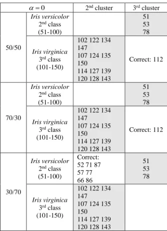
In the first experiment with original Iris data for all initial partitions for three classes, we correctly separate the 1st
class and decrease errors in separation of intersecting 2nd
and 3rd classes (Table 1, Fig.1). For two intersecting
clas-ses only, we decrease errors in the separation of the 2nd and
3rd classes, too (Table 1, Fig. 2, 3). It can be seen that the
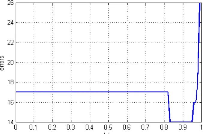
optimal intervals for * depend on the number of clusters (Table 1), hence on data dispersion, and can slightly differ for different initial partitions. Error diagrams are not mon-otonic functions (Fig. 1–3).
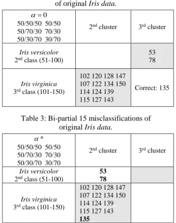
As we can see, original Iris data are some sort of “well structured” data, since for different initial partitions we get the same 16 misclassified objects for the classical (=0) criterion and the same 15 misclassified objects for the bi-partial ( *) criterion (Table 1). For the classical criterion, misclassified objects are generally from the 3rd class
(Ta-ble 2). The object 135 is well classified and shown here, since it is misclassified for the bi-partial criterion.
Misclassified objects for the bi-partial criterion are from the 3rd class, too (Table 3). Here, objects 53 and 78
are well classified, and the object 135 is misclassified. We repeat this experiment for standardized data (Ta-ble 4). Such data are more complicated. As we know, Iris
classes are not so spherical ones in the original feature space, and that is why the k-means type of approach is not the best suited for them.
After data standardization, classes appear to be more spherical and contain more “mixed” objects from inter-secting classes, usually giving more misclassifications in the classical case (Table 4).
Hence, for the classical criterion (=0) for standard-ized data, 25 misclassified objects are from two intersect-ing classes, 2nd and 3rd, with well classified all objects
from the 1st class (Table 5). Objects 104, 109, 112, 126,
129 are well classified and shown too, since they are mis-classified for the bi-partial criterion.
Misclassified objects for the bi-partial criterion are mainly from the 3rd class again (Table 6). Here, objects 52,
57, 66, 71, 76, 86, 87 are well classified and objects 104, 109, 112, 128, 129 are misclassified.
Table 1: Clustering results of original Iris data.
Initial partitions
Errors
(=0) *
Errors
( *) Diagrams 50/50/50 16 0.6 ÷ 0.75 15
Fig. 1 50/70/30 16 0.6 ÷ 0.75 15
50/30/70 16 0.6 ÷ 0.75 15 50/50 16 0.81 ÷ 0.92 15
Fig. 2 70/30 16 0.81 ÷ 0.92 15
30/70 16 0.81 ÷ 0.91 15 Fig. 3
Table 2: Classical 16 misclassifications of original Iris data.
0 =
50/50/50 50/50 50/70/30 70/30 50/30/70 30/70
2nd cluster 3rd cluster
Iris versicolor
2nd class (51-100)
53 78
Iris virginica
3rd class (101-150)
102 120 128 147 107 122 134 150 114 124 139 115 127 143
Correct: 135
Table 3: Bi-partial 15 misclassifications of original Iris data.
* 50/50/50 50/50 50/70/30 70/30 50/30/70 30/70
2nd cluster 3rd cluster
Iris versicolor
2nd class(51-100)
53 78
Iris virginica
3rd class(101-150)
102 120 128 147 107 122 134 150 114 124 139_ 115 127 143 135_
Table 4: Clustering results of standardized Iris data.
Initial partitions
Errors
(=0) *
Errors
( *) Diagrams
50/50/50 25 0.85 22
Fig. 4
50/70/30 25 0.85 22
50/30/70 25 0.85 22
50/50 17 0.94 ÷ 0.97 15 Fig. 5
70/30 17 0.92 ÷ 0.97 15 Fig. 6
Table 5: Classical 25 misclassifications of standardized Iris data.
0 =
50/50/50 50/70/30 50/30/70
2nd cluster 3rd cluster
Iris versicolor
2nd class(51-100)
51 57 76 86 52 66 77 87 53 71 78
Iris virginica
3rd class(101-150)
102 120 134 147 107 122 135 150 114 124 139 115 127 143
Correct: 104 129 109 112 128
Table 6: Bi-partial 22 misclassifications of standardized Iris data.
* 50/50/50 50/70/30 50/30/70
2nd cluster 3rd cluster
Iris versicolor
2nd class(51-100)
52 71 86 57 76 87 66 77
51 53 78
Iris virginica
3rd class(101-150)
102 122 139 104 107 124 143 109 114 127 147 112 115 134 150 128 120 135 129 Table 7: Classical 17 misclassifications
of standardized Iris data.
0
= 2nd cluster 3rd cluster
50/50
Iris versicolor
2nd class
(51-100)
51 53 78
Iris virginica 3rd class
(101-150)
102 122 134 147 107 124 135 150 114 127 139 120 128 143
Correct: 112
70/30
Iris versicolor
2nd class
(51-100)
51 53 78
Iris virginica 3rd class
(101-150)
102 122 134 147 107 124 135 150 114 127 139 120 128 143
Correct: 112
30/70
Iris versicolor
2nd class
(51-100)
Correct: 52 71 87 57 77 66 86
51 53 78
Iris virginica 3rd class
(101-150)
102 122 134 147 107 124 135 150 114 127 139 120 128 143
Table 8: Bi-partial misclassifications of standardized Iris data.
*
2nd cluster 3rd cluster
50/50
Iris versicolor
2nd class
(51-100)
51 53 78
Iris virginica 3rd class
(101-150)
102 122 134 147 107 124 135 150 114 127 139 120 128 143 112
70/30
Iris versicolor
2nd class
(51-100)
51
53 78
Iris virginica 3rd class
(101-150)
102 122 134 147 107 124 135 150 114 127 139 120 128 143
30/70
Iris versicolor
2nd class
(51-100)
52 71 87 57 77 66 86
51 52 71 87 53 57 77 78 66 86
Iris virginica 3rd class
(101-150) 107 114 120 135
102 128 147 122 134 150 124 139 127 143
For two intersecting classes of standardized data and for the classical (=0) criterion (Table 7), we get the same 3 misclassified objects from the 2nd class and 14
mis-classified objects from the 3rd class.
We get different misclassified objects (Table 8) for different initial partitions in the bi-partial case (15 objects for the 50/50 and 70/30 initial partitions, 14 objects for the 30/70 initial partition).
For standardized data, we usually get different results for three and two classes relative to original data. As we can see, the best result with the minimum of 14 errors for the initial partition 30/70 differs in terms of objects from the results for other initial partitions (Table 8).
Even though standardization is a usual step in data pro-cessing, we can see that the clustering results for standard-ized Iris data are not so “natural” as for the original ones. This is the well known and unwanted effect of standardi-zation.
Clustering results for Iris data by both classical and by bi-partial criteria are more “natural” for original data than for standardized data.
In the second experiment, we investigate the already mentioned general defect of the criterion (1). As it is well known, the classical k-means clustering tries to get clus-ters, which are approximately equal by size.
In case of classes that differ as to their sizes, the new permutable algorithm decreases usually the size of the big-ger class (2nd and 3rd together) and increases the size of the
smaller class (1st).
This is the classical result for
=0 with three errorsFigure 1. Clustering errors of original Iris data for Se-tosa/Versicolor/Virginica varieties (50/50/50, 50/70/30, 50/30/70) with 15 misclassified objects.
Figure 2. Clustering errors of original Iris data for Ver-sicolor/Virginica varieties (50/50, 70/30) with 15 misclas-sified objects.
Figure 3. Clustering errors of original Iris data for Ver-sicolor/Virginica varieties (30/70) with 15 misclassified objects.
Figure 4. Clustering errors of standardized Iris data for Setosa/Versicolor/Virginica varieties (50/50/50, 50/70/30, 50/30/70) with 22 misclassified objects.
Figure 5. Clustering errors of standardized Iris data for Versicolor/Virginica varieties (50/50) with 15 misclassi-fied objects.
Figure 7. Clustering errors of standardized Iris data for Versicolor/Virginica varieties (30/70) with 14 misclassi-fied objects.
Figure 8: Clustering errors of original Iris data for Setosa versus Versicolor/Virginica varieties (50/100, 100/50, 30/120).
We reduce errors to zero (Fig. 8) and correctly separate the smaller 1st class from the bigger one (2nd and 3rd) in the
optimal interval 0.97
* 1 for all initial partitions, i.e. 50/100, 100/50, 30/120. For standardized data, the result contains no errors at all for the whole interval 0
1for all initial partitions.
6
Conclusion
The k-means procedure is very popular in machine learn-ing and data minlearn-ing fields. This procedure is very natural and understanding its principles and results is easy. Addi-tionally, this procedure is deeply connected with other ideas, like the EM-algorithm, SOMs, etc.
On the other hand, the use of the bi-partial criterion can improve the classical clustering result. The bi-partial ob-jective function consists of two parts, the first one support-ing the best approximation of individual categories, and the second one supporting the appropriate separation among the categories. In the case of the k-means algo-rithm, the bi-partial objective function combines intra-cluster dispersions with the inter-intra-cluster similarity, to be jointly minimized. In dual form, the bi-partial objective function combines cluster concentrations with the inter-cluster dispersion, to be maximized.
In this paper, we investigate the direct form of the bi-partial criterion function. The first part of this criterion provides the classical quality measure of k-means cluster-ing, based on distances between objects.
As it is shown in this paper, the bi-partial criterion does not work directly through the standard procedure of the classical k-means, since the second part of the criterion cannot be changed within the classical procedure.
Therefore, to improve the clustering quality based on the bi-partial criterion, we develop here the new permuta-ble version of the classical k-means algorithm.
As it is shown in this paper, the permutable k-means appears to be a new type of clustering procedures.
The permutable k-means uses distances and similari-ties only. Therefore, it does not need to use the feature-based representation of experimental data. To reduce the computational complexity of permutations we can use in further work the optimal iterative techniques.
It is easy to show that in the dual form the bi-partial objective function combines cluster concentrations with the inter-cluster dispersion, to be jointly maximized. The first part of both bi-partial objective functions provides the “standard” quality of clustering based on distances be-tween objects (the classical k-means) or similarities be-tween them in dual form (the similarity k-means).
As a result, what the algorithm have we built? It is clear, that we have merely shown the principle of devel-oping a class of criteria and corresponding algorithms. As we can see in Figs. 1–7, error lines are not convex func-tions of in general. The future study should, then, be oriented at defining conditions for convexity, on the one hand, and developing effective algorithms of extrema finding of the similar functions, on the other.
Acknowledgements
The work of the first author was supported by Russian Foundation for Basic Research under grant 17-07-00319.
References
[1] H. Steinhaus (1956). Sur la division des corps maté-riels en parties. Bulletin de l’Academie Polonaise des
Sciences IV (C1.III), 801-804 (in French).
[2] M.I. Shlezinger (1965). Spontaneous discrimination of patterns. In: Reading Automata. Naukova Dumka, Kiev (in Russian).
[3] M.I. Shlezinger (1968). The interaction of learning and self-organization in pattern recognition. In: Kibernetika, 4(2), 81-88. http://irtc.org.ua/image/ Files/Schles/non-supervised.pdf
[4] A.V. Milen’kii (1975). Classification of signals in conditions of uncertainty. Moscow, Soviet Radio (in Russian).
[5] E. Diday et al. (1979). Optimisation en classification
automatique. INRIA, Domaine de Voluceau,
Rocquencourt B.P. 105, 78150 Le Chesnay (in French).
[6] W.S. Torgerson (1958). Theory and Methods of Scaling. N.Y., Wiley.
[8] H. Späth (1983). Cluster-formation und -analyse:
Theorie, FORTRAN-Programme und Beispiele.
R. Oldenbourg-Verlag, München — Wien.
[9] S.A. Aivazyan, et al. (1989). Applied Statistics. Classification and reduction of dimensionality (Ch. 5. Basic concepts and definitions used in classi-fication without training. 5.4. Classiclassi-fication quality functionals and extremal approach to cluster analy-sis problems). Finansy i statistika, Moscow (in Rus-sian)
[10] H.-J. Mucha, U. Simon, R. Brüggemann (2002).
Model-based Cluster Analysis Applied to Flow
Cy-tometry Data of Phytoplankton. Tech. Report,
Ber-lin. http://www.wias-berBer-lin.de/techreport/5/ wias_technicalreports_5.pdf
[11] E. Pekalska, R.P.W. Duin (2005). The Dissimilarity Representation for Pattern Recognition. Founda-tions and ApplicaFounda-tions. W.S. Singapore.
[12] A.W.F. Edwards, L.L. Cavalli-Sforza (1965). A Method for Cluster Analysis. In: Biometrics, 21, 362–375. https://www.jstor.org/stable/ 2528096 ?seq=1#page_scan_tab_contents
[13] Jan W. Owsinski (2012). On the optimal division of an empirical distribution (and some related prob-lems). In: Przegląd Statystyczny, special issue, 1, 109-122.
[14] Jan W. Owsinski (2013). On dividing an empirical distribution into optimal segments. http://new.sis-statistica.org/wp-content/uploads/ 2013/09/RS12-On-Dividing-an-Empirical-Distribution-into.pdf [15] Jan W. Owsinski (2011). The bi-partial approach in
clustering and ordering: the model and the algo-rithms. In: Statistica & Applicazioni. Special Issue, 43–59.
[16] Jan W. Owsinski (1990). On a new naturally indexed quick clustering method with a global objective function. In: Applied Stochastic Models and Data Analysis, 6(3), 157-171.
https://doi.org/10.1002/asm.3150060303
[17] S.D. Dvoenko (2009). Clustering and separating of a set of members in terms of mutual distances and sim-ilarities. In: Transactions on MLDM. IBaI Publish-ing 2, 2 (Oct. 2009), 80-99.
[18] S. Dvoenko (2014). Meanless k-means as k-meanless clustering with the bi-partial approach. In: Proc. of 12th Int. Conf. on Pattern Recognition and Image
Processing (PRIP’2014). UIIP NASB, Minsk,
Bela-rus, 50-54.
[19] R.O. Duda, P.E. Hart (1973). Pattern Classification and Scene Analysis. N.Y., Wiley.
[20] R.O. Duda, P.E. Hart, D.G.Stork (2000). Pattern
Classification. Wiley-Interscience New York, NY.
[21] R.A. Fisher (1936). The use of multiple measure-ments in taxonomic problems. In Ann. Eugenics. 7, 2 (Sept. 1936), 179-188.
https://doi.org/10.1111/j.1469-1809.1936.tb02137.x [22] S. D. Dvoenko, D.O. Pshenichny (2016). A recov-ering of violated metric in machine learning. In: Pro-ceedings of 8th Int. Symposium on Information and
Communication Technology (SoICT’2016). ACM
NY, 15-21.