Vol. 8, No. 1, 2015, 26-49
ISSN 1307-5543 – www.ejpam.com
Modeling, Simulation and Performance Analysis of a Flexible
Production System
Mohamed Boualem
1, Mouloud Cherfaoui
2, Amina Angelika Bouchentouf
3,∗, Djamil
Aïssani
11Research Unit LaMOS (Modeling and Optimization of Systems), Faculty of Technology, University
of Bejaia, 06000 Bejaia, Algeria
2Research Unit LaMOS (Modeling and Optimization of Systems) University of Bejaia, 06000 Bejaia,
Algeria
Department of Mathematics, University of Biskra, 07000 Biskra, Algeria.
3Mathematics Laboratory, Department of Mathematics, Djillali Liabes University of Sidi Bel Abbes,
89, Sidi Bel Abbes 22000, Algeria.
4Research Unit LaMOS (Modeling and Optimization of Systems), Faculty of Exact Sciences,
Univer-sity of Bejaia, 06000 Bejaia, Algeria.
Abstract. This paper deals with a flexible production system modeled by re-entrant queueing network; a system decomposed into two fundamental multi-productive stations and three classes, a part follows the route fixed by the system, where each one is processed first by station 1 for the first step, then by station 2 for the second step, and again by the first station for third and last step before leaving the system. We assume that there is an infinite supply of work available, so that there are always parts ready for processing step 1, and that the first station gives preemptive priority to buffer 3.
Several performance measures have been used to evaluate the system performances considering two scenarios; high priority with service conservation and high priority with loss of parts. So, performances due to varying its parameters are investigated through expanded Monte Carlo simulations.
2010 Mathematics Subject Classifications: 60K25, 68M20, 90B22
Key Words and Phrases: Queueing models; flexible production systems; modeling; simulation; stabil-ity.
1. Introduction
Flexible production systems have emerged as one of the revolutions in the production industries in recent years. It has made it possible to produce a vast variety of parts in less time and cost.
∗Corresponding author.
Email addresses:[email protected](M. Boualem),[email protected](M. Cherfaoui),[email protected](A. Bouchentouf),[email protected](D. Aïssani)
These systems are generally consisting in a number of machine tools, robots, material handling, automated storage and retrieval system, and computers or workstations. A typical flexible production system can fully process the members of one or more part families on a continuing basis without human intervention.
Over the last few decades, the modeling and the analysis of flexible production systems has been meticulously studied by control theorists and engineers.
The case study in the present paper mainly consists of modeling, simulation and analysis of a flexible production system.
Modeling and simulation of flexible production systems is a field of research for many people now days. However, they all share a common aim; to search for solutions to attain higher speeds and more flexibility and thus maximize/multiplicate manufacturing productivity. Computer simulation is a great numeric modeling technique for the analysis of flexible manufacturing/product systems. Bruccoleriet al. [5] suggested the simulation as a tool for defining the configuration of an flexible manufacturing system. Shnitset al. [29] used sim-ulation of operating system as a decision support tool for controlling the flexible system to exploit flexibility. Tüysüz and Kahraman[30] presented an approach for modeling and anal-ysis of time critical, dynamic and complex systems using stochastic Petri nets together with fuzzy sets.
Many other authors used Petri net approach to analyze and present the Performance eval-uation of complex manufacturing systems, for simultaneously modeling and scheduling man-ufacturing systems for instance Liuet al. [22], Huanget al. [19], Delgadillo and Llano[14].
In this research work, flexible production system is modeled by a reentrant queueing sys-tem to analyze its performance measures. In addition, we compare and verify the results obtained from the simulation techniques and theoretical results given for this type of systems. Stability and performance analysis of multi-class queueing networks is by now a well-researched field. Some preeminent papers which have set the accent of this research field in the past 25 years are many, some of them are[7, 8, 18, 20]. Some notorious contributions with respect to stability analysis can be summarized in[3, 11, 15, 25, 28], additional contributions are summarized in[4, 10, 24].
Let us note that the re-entrant lines (described in Harrison [18]) are a special case of queueing systems that can be used to model complex manufacturing system such as wafer fabrication facilities. Kumar [20] defined these systems called standard re-entrant lines for convenience.
stream as the output of a server which is fed by an infinite supply of work.
Infinite supply of work and infinite virtual queues are discussed in[1, 2, 17, 27, 31, 32]. A succinct study of these results is given in[26].
The layout of our paper is as follow; after an introduction, a mathematical model of the production system is described in Section 2. Section 3 presents some theoretical results given for such model, Section 4 is devoted to the simulation approach study. In Section 5 a general conclusion is offered.
2. Mathematical Model
2
1
3
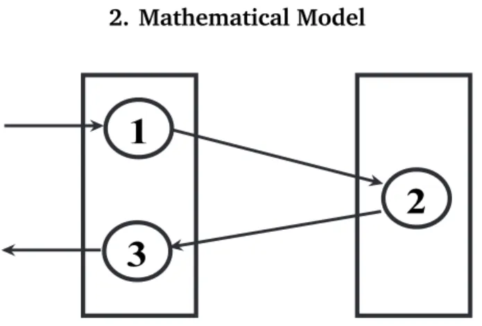
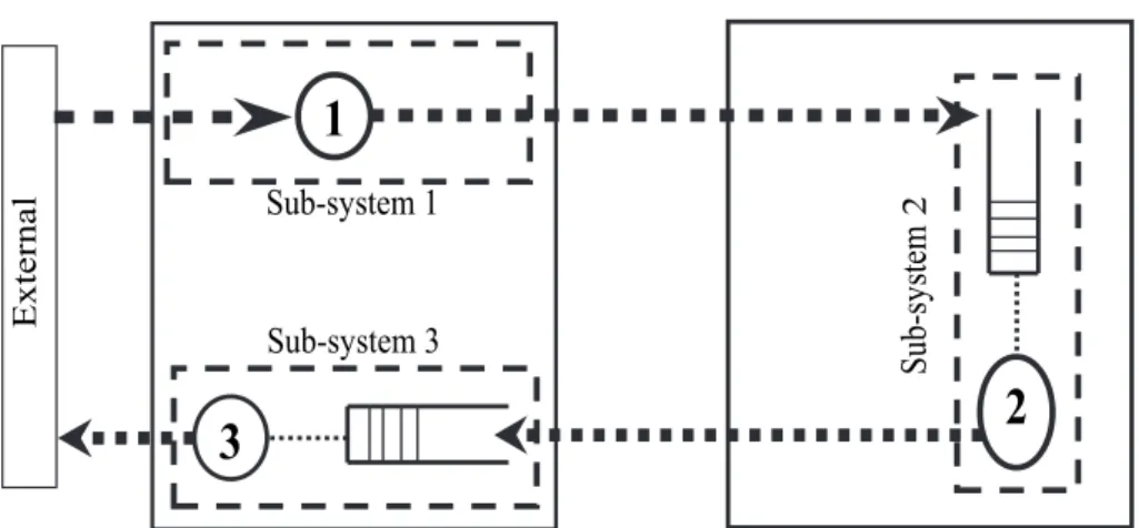
Figure 1: A Reentrant Network with Two Stations and Three Classes
The production system considered in our study is schematically shown in Figure 1. This process can be seen as a reentrant queueing network, consisting of two stations and three classes. Parts arrive according to a Poisson process with rateλ. When the part arrives at the first station, if it finds some ones before it, it waits in the queue 1, otherwise it goes directly to the service to be served with rateµ1, then aligns the second line requiring a second service with rateµ2. Finally, the part returns to the first station for the third and final service before leaving the system. Indeed, there are three types of parts, parts of classC1 processed by the first station for the first service, parts of classC2processed by the second station for the second service and parts of the classC3 processed by the first station for the third and final service.
We assume that there is an infinite supply of work available, so that there are always parts ready for processing step 1. In that case station 1 will always be busy. Each class is processed in FIFO order. Processing is non-idling, that is a station will always process a part when there is work. The present research work consider two scenarios.
2 into class 3, station 1 will preempt its work at class 1, and immediately starts processing class 3.
In the second scenario, each part which arrives to the system, is lost if it is not at the head of the queue, it will be also lost if it is interrupted by the arriving parts from station 2 to class 3.
3. Theoretical Study
Queueing systems are excessively useful class models that have found application in many areas including communication networks, computer systems, manufacturing. . . Much of this success is maybe due to the constitutional tractability of a large class of queueing systems. However, the question of stability of many queueing systems and their performance evalua-tion are extremely exchanging issues. Stability analysis and performance evaluaevalua-tion of queu-ing systems have received a great deal of attention, this is partly due to several examples that demonstrate that the usual conditions; traffic intensity less than one at each station (ρi <1) are not sufficient for stability, even under the well known FIFO service discipline (Dai and Vande Vate [12]). Rybko and Stolyar [28] and Lu and Kumar[23] demonstrated that in a deterministic version the usual conditions do not guarantee the stability of many queueing networks. Dai[11]provided a unified approach via fluid limit model to prove positive Harris recurrence of a network with two stations and N classes with feedback. Thereafter, Dai and Weiss[13]gave sufficient conditions for the re-entrant line to be stable (global stability) what-ever the discipline of service. Chen and Zhang[9] have established sufficient conditions for the stability of multi-class queueing networks under FIFO service discipline. Weiss[31] stud-ied a reentrant network with two stations and three classes with an infinite supply of work under LFBS service discipline (Last Buffer First served), where arrivals are not random and the service times are exponential with meanmi for each classi.
The stability conditions associated with our production system are those removed from the model studied by Weiss[31]. Indeed, the purpose of his work revolves around the following question: Under what conditions on the system parameters, the Markov process reaches the steady state ?
So, we assume that there is an infinite supply of work available, we analyze this system under the LBFS policy: station 1 gives priority to parts in class 3 over parts in class 1, we assume that this priority is preemptive; whenever a part arrives in class 3, station 1 will preempt the part in class 1 and start processing the part in class 3, and it will resume work on the part in class 1 only when class 3 is empty.
Let note that in general, it is well know that if parts arrive at this system in a renewal stream, at rateλ, then under the conditionρ1=λ(m1+m3)<1, andλm2<1 the queues of parts waiting for each step are stable, and in fact the system is positive Harris recurrent, for any work conserving policy, readers are referred to Kumar and Kumar[21]and Dai and Weiss
[13], for more details.
weakly to infinity. Consequently such a system cannot work at a rate max{ρ1,ρ2}=1, without accumulating unbounded queues.
Weiss[31], established a sufficient condition for the stability for such system. So if
λµ1
1 +
1
µ3
> αµ1
2 then under LBFS policy ρ1 =1, but the queues for steps 2 and 3 will be
stable, and the system will be positive recurrent.
Theorem 1([31]). If
λ
1
µ1 +
1
µ3
> α 1
µ2, (1)
then the system is recurrent positive.
Adan and Weiss [1]kept considering the caseλµ1
1 +
1
µ3
> αµ1
2; station 1 works all the
time and the system is weakly stable, then by solving the balance equations of such system a stationary distribution network is obtained.
Guo and Zhang[17]obtained sufficient and necessary condition for the stability for such network.
Guo[16]using a fluid model approach, obtained a sufficient condition for the model con-sidered. In addition, the author got necessary conditions for the corresponding fluid model to be weakly stable.
Proposition 1. [16]If
ρ2>1, (2)
the the fluid model is weakly stable. Thus the reentrant network is unstable.
Yoni Nazarathy and Gideon Weiss [27] considered the same model given in Weiss[31], and proposed a method for the control over a finite time horizon, the model was approximated by a fluid network and formulated a fluid optimization problem. The optimal fluid solution partitions the time horizon to intervals in which constant fluid flow rates were maintained. Then, they used a policy by which the queueing network tracks the fluid solution. To that end, they modeled the deviations between the queueing and the fluid network in each of the intervals by a multi-class queueing network with some infinite virtual queues. These deviations were kept stable by an adaptation of a maximum pressure policy.
Now, let us note that from previous results, one leads to the following consequence.
Consequence 1. Consider the network presented in Figure 1, if
ρ1=λ
1
µ1 +
1
µ3
<1, (3)
ρ2= λ
µ2 <1, (4)
ρ1>ρ2, (5)
4. Simulation Study Approach
Performance analysis of any system is one of the most studied topics in Operations Re-search. In practice, we are often interested in numbers of customers in the system and their waiting time.
However, the expression of these performances depends heavily on how customers arrive to the system, the manner on which customers request services and service disciplines. To control them, we are led to the problem by modeling these systems via queueing models.
So, a queueing network is a set of interconnected queues, at which circulate one or more classes of customers. Two important parameters (generally stochastic) determine the behavior of the network (open or closed network) over the time:
• The inter-arrival times of customers. • The service times.
The main objective of this work is to model the production line, to analyze, to evaluate and improve its performance using computer simulation techniques. Finally, conclusions are drawn from the analysis made and then recommendations are given based on those concluded points.
Therefore, it is believed that the work will add some value to the existing knowledge. Analysis and evaluation of a production system usually uses performance indicators capa-ble of assessing the adequacy of the model used with respect to the real system. We first start by specifying performance measures which we consider interesting to study:
• Mean number of customers in the overall systemN and in each sub-systemNi,i=1, 3.
• Mean number of customers waiting in the overall systemQ and in each sub-systemQi,
i=1, 3.
• Total load of the overall systemρC and the load of each sub-systemρC
i,i=1, 3.
Our main goal is to evaluate these performance measures, via Monte Carlo simulation technique for the network described in Section 2 considering two scenarios:
Scenario 1: Station 1 gives preemptive priority toC3, when this latter empties, station 1 will instantaneously resume processing of a part in step 1.
Scenario 2: Station 1 gives preemptive priority to C3, and customer of class 1 is lost if it is
not at the head of the queue, it will be also lost if it is interrupted by the arriving customer from station 2 toC3.
To this end, we develop a simulation algorithm under MATLAB at discrete event. The latter allows us to have two types of results:
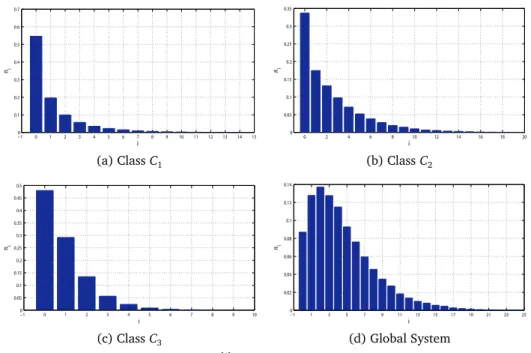
Graphical results: Representation of the stationary probabilities of the states of the overall system and subsystems, depending on its parameters. The abscissa axis represents the number of customerskin the system (respectively,kiin theithsub-system,i=1, 3) and
the ordinate axis represents the stationary probabilityπk having k parts in the system (respectively,π(ki)
i in thei
thsub-system), wherek= P3
i=1
ki.
Subsequently, we analyze the influence of parameters of the considered systems (Scenario 1 and Scenario 2), by varying the arrival and service ratesλ (resp. µi, i =1, 3), after that, we determine some values of parametersρj, j=1, 2 which are in terms ofλandµi, to check whether the stability conditions of such systems described by the inequalities (3), (4) and (5) are fulfilled. Firstly, we fix the service rate (µi,j = 1, 3) and let varying the arrival rate
λ. Secondly, the procedure is taken inversely (we fixλand let varying µi,i=1, 3), so as to obtain the different states of the network (stable, unstable, weakly stable).
5. First scenario: Results and Discussion
In this part, we suppose that when the third class is emptyn3=0, parts are processed out
of class 1 andn2 increases until the second station completes the processing of a part out of it class at which time the state is(n2−1, 1), and station 1 switches to class C3 at that time
customers of classC1 are interrupted, the interrupted customer joins the QRIC queue (queue
of capacity 1 reserved for interrupted customer).
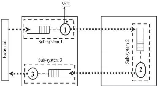
While classC3 is not empty, parts arrive at classC3from classC2at rateµ2and depart out of classC3at rateµ3, so classC3behaves like anM/M/1 queue, except that the total number
of arrivals into classC3 cannot exceedµ2. Mathematical model associated with this network is shown in Figure 2.
1
2
3
Sub-system 3 Sub-system 1
Sub-s
ys
tem
2
External
QRIC
5.1. Variation of the Parameter
λ
Let T ma x =10000 time units be the simulation duration andM C =100 the number of replications. Forµi = 1/3, (i = 1, 3), we varyλ (λ = [0.10, 0.13, 0.16, 0.17]). The mean number of customers in the sub-systems, in the overall system and the in the queues as the loads are mainly summarized in the Tables 1, 2 and 3.
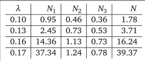
Table 1: Variation ofN andNi in Terms ofλ
λ N1 N2 N3 N
0.10 0.95 0.46 0.36 1.78
0.13 2.45 0.73 0.53 3.71
0.16 14.36 1.13 0.73 16.24 0.17 37.34 1.24 0.78 39.37
Table 2: Variation ofQandQi in Terms ofλ
λ Q1 Q2 Q3 Q
0.10 0.47 0.16 0.06 0.70
0.13 1.75 0.34 0.14 2.24
0.16 13.43 0.66 0.26 14.36 0.17 36.37 0.75 0.29 37.41
Table 3: Variation ofρC andρC
i in Terms ofλ
λ ρC
1 ρC2 ρC3 ρC
0.10 47.50 30.13 29.70 73.53 0.13 69.53 38.94 39.16 88.35 0.16 92.72 47.42 47.63 97.89 0.17 97.83 49.20 49.22 99.44
5.2. Discussion of Results
From Tables 1, 2 and 3, we remark that:
Ø The mean number of customers in the system and in the queue of each sub-system in-creases with respect toλ. The number of customers increases significantly in the sub-system 1 compared to subsub-systems 2 and 3, which generates a big number of customers in the queue 1 and the overall system. The overall system load increases in terms ofλ
(loads of subsystems 2 and 3 are nearly equal in all cases).
which indicates that there is a smooth transit from a sub-system to another, which means that customers are not blocked at any sub-system. In addition, the load of the overall system isρC≤90% (the system is stable, because of the stability conditions given in (1) are verified).
Ø Forλ≥0.16, the system load is considerable(ρC>97%)which is generated by a high load at the first sub-system (ρC
1 ≥ 92%). Moreover, when λ increases (from 0.16 to
0.17), the network moves from stability to instability because of the the first station. While the loads of the two subsystems 2 and 3 are average.
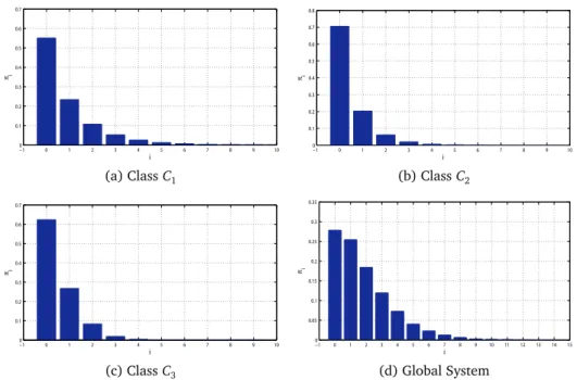
Ø A significant difference between the mean number of customers in the 1st sub-system and subsystems 2 and 3, because of blocked customers of class C1, caused by the high priority given to the classC3 and the service rate which is below the arrival rate. Figures 3 and 4 represent the stationary probabilities of the states of the network forλ=0.1 andλ=0.17; we conclude that:
Ø Moreλincreases, more the probability that the system is empty decreases (π0). Unlike the stability case (Figure 3), the probabilityπ0is almost negligible in the instability case (Figure 4 for the caseλ=0.17).
Ø The probability that it would have a very large number of customers in the first sub-system, πk
1, is considerable (Figure 4), the station 1 is saturated. Consequently, the
global system becomes saturated, this is due to the fact that the first condition of stability is not verified(ρ1=1.02).
−1 0 1 2 3 4 5 6 7 8 9 10 0 0.1 0.2 0.3 0.4 0.5 0.6 0.7 i πi
(a) ClassC1
−1 0 1 2 3 4 5 6 7 8 9 10
0 0.1 0.2 0.3 0.4 0.5 0.6 0.7 0.8 i πi
(b) ClassC2
−1 0 1 2 3 4 5 6 7 8 9 10
0 0.1 0.2 0.3 0.4 0.5 0.6 0.7 i πi
(c) ClassC3
−1 0 1 2 3 4 5 6 7 8 9 10 11 12 13 14 15 0 0.05 0.1 0.15 0.2 0.25 0.3 0.35 i πi
(d) Global System
Figure 3: Stationary Probabilitiesπ(ki)
0 20 40 60 80 100 120 140 160 180 200 0
0.005 0.01 0.015 0.02 0.025
i
πi
(a) ClassC1
−1 0 1 2 3 4 5 6 7 8 9 10 11 12 13 14 15 0
0.1 0.2 0.3 0.4 0.5 0.6 0.7
i πi
(b) ClassC2
−1 0 1 2 3 4 5 6 7 8 9 10 0
0.05 0.1 0.15 0.2 0.25 0.3 0.35
i πi
(c) ClassC3
0 20 40 60 80 100 120 140 160 180 200
0 0.002 0.004 0.006 0.008 0.01 0.012 0.014 0.016 0.018
i
πi
(d) Global System
Figure 4: Stationary probabilitiesπ(ki)
i andπk forλ=0.17 andµi=1/3
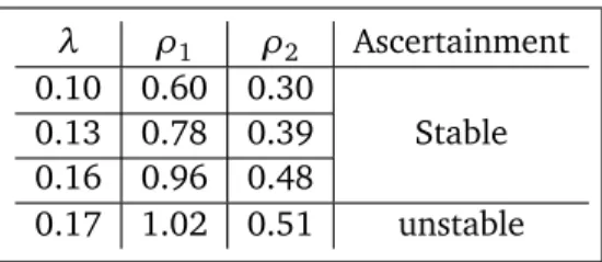
Table 4 summarizes the results carried out previously. Essentially, we can say that the network is unstable if at least one of the necessary conditions (ρ1<1 andρ2<1) is unverified. Furthermore, the stability is not achieved if the following three conditions is violated:ρ1<1,
ρ2<1 andρ1> ρ2.
Table 4: Summary, whenλVaries
λ ρ1 ρ2 Ascertainment
0.10 0.60 0.30
0.13 0.78 0.39 Stable
0.16 0.96 0.48
0.17 1.02 0.51 unstable
5.3. Variation of Service Rates
µ
1and
µ
3Let varying the service ratesµ1 andµ3, and fixe the arrival rate λ=0.10 andµ2=0.15.
Table 5: Variation ofN andNi in Terms of(µ1,µ3)
µ1 µ3 N1 N2 N3 N
0.75 0.10 61.58 6.25 4.33 72.16
0.70 0.15 3.29 3.44 1.50 8.24
0.65 0.20 1.25 2.40 0.84 4.49
0.60 0.25 0.80 2.24 0.59 3.64
0.55 0.30 0.63 2.18 0.46 3.28
0.50 0.35 0.57 2.09 0.37 3.04
0.45 0.40 0.55 2.10 0.32 2.98
0.44 0.41 0.55 1.97 0.30 2.84
0.40 0.45 0.59 2.07 0.28 2.94
0.35 0.50 0.63 1.97 0.24 2.85
0.30 0.55 0.76 1.96 0.21 2.95
0.25 0.60 1.00 2.00 0.19 3.20
0.20 0.65 1.53 2.05 0.18 3.76
0.15 0.70 3.69 2.00 0.16 5.86
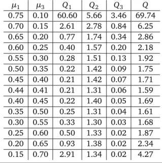
Table 6: Variation ofQandQi in Terms of(µ1,µ3)
µ1 µ3 Q1 Q2 Q3 Q
0.75 0.10 60.60 5.66 3.46 69.74
0.70 0.15 2.61 2.78 0.84 6.25
0.65 0.20 0.77 1.74 0.34 2.86
0.60 0.25 0.40 1.57 0.20 2.18
0.55 0.30 0.28 1.51 0.13 1.92
0.50 0.35 0.22 1.42 0.09 1.75
0.45 0.40 0.21 1.42 0.07 1.71
0.44 0.41 0.21 1.31 0.06 1.59
0.40 0.45 0.22 1.40 0.05 1.69
0.35 0.50 0.25 1.31 0.04 1.61
0.30 0.55 0.33 1.30 0.03 1.68
0.25 0.60 0.50 1.33 0.02 1.87
0.20 0.65 0.93 1.38 0.02 2.34
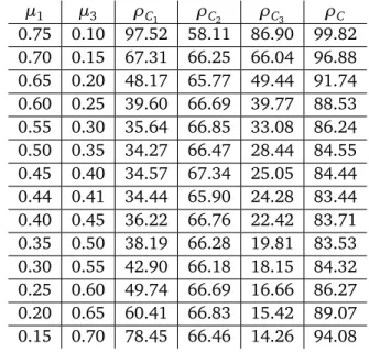
Table 7: Variation ofρC andρC
i in Terms of(µ1,µ3)
µ1 µ3 ρC
1 ρC2 ρC3 ρC
0.75 0.10 97.52 58.11 86.90 99.82
0.70 0.15 67.31 66.25 66.04 96.88
0.65 0.20 48.17 65.77 49.44 91.74
0.60 0.25 39.60 66.69 39.77 88.53
0.55 0.30 35.64 66.85 33.08 86.24
0.50 0.35 34.27 66.47 28.44 84.55
0.45 0.40 34.57 67.34 25.05 84.44
0.44 0.41 34.44 65.90 24.28 83.44
0.40 0.45 36.22 66.76 22.42 83.71
0.35 0.50 38.19 66.28 19.81 83.53
0.30 0.55 42.90 66.18 18.15 84.32
0.25 0.60 49.74 66.69 16.66 86.27
0.20 0.65 60.41 66.83 15.42 89.07
0.15 0.70 78.45 66.46 14.26 94.08
5.4. Discussion of Results
According to the numerical results stored in Tables 5, 6 and 7, we observe that:
Ø Forµ1=0.75 andµ3 =0.10, the mean number of customers in the first sub-system is very large compared to subsystems 2 and 3. Therefore, the network is unstable, because of(ρ1>1).
Ø Forµ1andµ3which vary respectively from 0.45 to 0.75 and from 0.10 to 0.40, the mean number of customers in the sub-system 1 decreases. As against, forµ1varying from 0.15 to 0.40 andµ3 from 0.45 to 0.70, the mean number of customers in the sub-system 1 increases. This situation is due because of high priority given toC3overC1.
Ø When the service rate of class C3 is less than service rate of class C1, the interrupted
customers of class 1 resume their services within a short time, which justifies the decrease in the number of customers in the 1stsub-system, and the converse is true.
Ø Forµ1=0.70 andµ3=0.15, the mean number of customers in each subsystems and the loads are distributed equitably. In addition, the arriving customers are served at the end of the simulation time, then the system is stable (all stability conditions are satisfied). Ø Forµ1 varying from 0.65 to 0.20 andµ3 varying from 0.20 to 0.65, the mean number
Ø Forµ1=0.15 andµ3=0.70, the system reaches the steady state as all stability condi-tions are fulfilled.
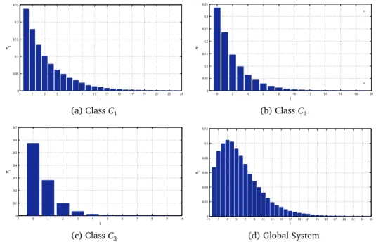
Details of some of results given in Tables 5, 6 and 7 are illustrated in Figures 5 and 6. When the service rate of classC3 is higher than the class C1, the probability of having 0 customer in the third sub-system is very high (equal almost to 1), the network is stable because all the conditions are fulfilled
−1 1 3 5 7 9 11 13 15 17 19 21 23 25
0 0.05 0.1 0.15 0.2 0.25
i
πi
(a) ClassC1
0 2 4 6 8 10 12 14 16 18 20
0 0.05 0.1 0.15 0.2 0.25 0.3 0.35
i
πi
(b) ClassC2
−1 0 1 2 3 4 5 6 7 8 9 10 0
0.1 0.2 0.3 0.4 0.5 0.6 0.7
i πi
(c) ClassC3
−1 1 3 5 7 9 11 13 15 17 19 21 23 25 27 29 31 33 35 0
0.02 0.04 0.06 0.08 0.1 0.12
i
πi
(d) Global System
Figure 5: Stationary Probabilitiesπ(ki)
i andπk forλ=0.10,µ1=0.15 andµ3=0.70
Figures 5 and 6, look the same. In Figure 6, the probability for having 0 customers in the third class decreases considerably, compared to that given in 5, because the service rate has declined (from 0.7 to 0.2). So the network converges to the steady state, but is not stable ((5) not verified).
−1 0 1 2 3 4 5 6 7 8 9 10 11 12 13 14 15 0 0.1 0.2 0.3 0.4 0.5 0.6 0.7 i πi
(a) ClassC1
0 2 4 6 8 10 12 14 16 18 20
0 0.05 0.1 0.15 0.2 0.25 0.3 0.35 i πi
(b) ClassC2
−1 0 1 2 3 4 5 6 7 8 9 10 0 0.05 0.1 0.15 0.2 0.25 0.3 0.35 0.4 0.45 0.5 i πi
(c) ClassC3
−1 1 3 5 7 9 11 13 15 17 19 21 23 25
0 0.02 0.04 0.06 0.08 0.1 0.12 0.14 i πi
(d) Global System
Figure 6: Stationary Probabilitiesπ(ki)
i andπk forλ=0.10,µ1=0.65 andµ3=0.20
Table 8: Summary, whenµ1 andµ3vary
µ1 µ3 ρ1 Ascertainment
0.75 0.10 1.33 unstable
0.70 0.15 0.80 weakly Stable 0.65 0.20 0.65
0.60 0.25 0.57 0.55 0.30 0.51 0.50 0.35 0.48
0.45 0.40 0.46 Stable
0.44 0.41 0.47 0.40 0.45 0.47 0.35 0.50 0.48 0.30 0.55 0.51 0.25 0.60 0.57 0.20 0.65 0.65
0.15 0.70 0.80 weakly Stable
5.5. Conclusion of the First Scenario
Ø While increasing the arrival rateλfrom 0.1 to 0.16(ρ1<1), the number of customers in the system increases gradually, especially in the station 1, but the system is stable as all the conditions are satisfied. Beyondλ=0.16, the sub-system 1 is saturated (ρ1>1), which causes the instability of the global network.
Ø We can see a change in performance while fixingµ2 and varyingµ1 andµ3 in interval
[0.15, 0.7]. The state of the network is greatly affected by the fluctuation service rate of the first station. Indeed, when λ = 0.01 and µ2 = 0.15, we get ρ2 < 1. These performance measures are the best whenµ3 < µ1, this is due to the priority given to customers of classC3. But for some values ofµ1 andµ3, for which the third condition is not verified, the system becomes weakly stable.
Finally, numerical results obtained by the simulation approach and the theoretical results shown by Weiss[31]correspond perfectly.
6. Scenario two: Results and Discussion
1
2
3
Sub-system 3 Sub-system 1
Sub-s
ys
tem
2
Ext
erna
l
Figure 7: The mathematical model (Scenario 2)
In this part, we study the stability and performance measures of the network described in Figure 2, considering the case of Loss customers (the interrupted customer leaves definitively the system), see Figure 7. Thus, when a customer arrives and finds the first station occupied by customer of classC3, it leaves the system (lost customer) in order to include the assumption of
perfect control of customers of classC1. Note that our scenario corresponds to the one given in
[2], except that in the latter, author has considered that processing of a part from class 1 only starts when class 3 is empty. However, once started machine 1 will complete the processing of step 1 of the part even if parts arrive in class 3 (after being processed by machine 2). As a result, if class 2 contains n2 parts and class 3 is empty, and processing of a part from class 1 starts, then at the end of the processing of step 1 of this part, there may be between 0 andn2
parts in class 3.
6.1. Variation of the Parameter
λ
In this experience, we fix the the service rate µi =1/3 (i=1, 3), and let varyingλfrom 0.01 to 0.17 with a pitch of 0.03. We keep the same input parameters as in the first experience (Scenario 1), let T ma x = 10000 time units be the simulation duration and M C = 100 the number of replications. The results obtained for this situation are stored in Tables 9, 10 and 11.
Table 9: Variation ofN andNi in Terms ofλ
λ N1 N2 N3 N
0.01 0.02 0.02 0.02 0.08
0.04 0.10 0.10 0.10 0.31
0.07 0.18 0.17 0.16 0.52
0.10 0.24 0.24 0.21 0.70
0.13 0.30 0.30 0.25 0.86
0.16 0.37 0.34 0.29 1.01
0.17 0.39 0.37 0.30 1.07
Table 10: Variation ofQandQi in Terms ofλ
λ Q1 Q2 Q3 Q
0.01 0.0009 0.0008 0.0005 0.002
0.04 0.011 0.011 0.005 0.03
0.07 0.03 0.03 0.01 0.07
0.10 0.05 0.05 0.02 0.13
0.13 0.08 0.07 0.03 0.20
0.16 0.12 0.10 0.04 0.27
0.17 0.13 0.11 0.05 0.29
Table 11: Variation ofρC andρC
i in Terms ofλ
λ ρ1 ρ3 ρC
1 ρC2 ρC3 ρC
0.01 0.06 0.03 2.87 2.83 2.79 8.38
0.04 0.24 0.12 9.67 9.66 9.74 27.55
0.07 0.42 0.21 15.01 14.87 14.99 41.12
0.10 0.60 0.30 18.94 18.83 18.77 50.26
0.13 0.78 0.39 22.08 22.36 22.11 57.68
0.16 0.96 0.48 24.91 24.76 24.90 63.43
6.2. Discussion of Results
From the results given in Tables 9, 10 and 11, we conclude that:
Ø The number of customers in the queue and in the system increases gradually in terms of
λ. Moreover, based on the important number of rejected customers of classC1, caused
by the high priority given to the classC3, the number of customers increases slightly. Ø For all values ofλ, all arriving customers to the network are served. This is due to the
fact that the mean number of customers in the system and the loads are almost the same in the three subsystems. In addition, the overall load never reaches a high level, even when the stability condition, given by the inequality (3) is not verified (ρC varies from 8.38%, (λ=0.01), to 65.05%, (λ=0.17)).
Ø The mean number of customers in the system and in the queue is small, compared to Scenario 1, for fixed values ofλ(λ=0.10,λ=0.13,λ=0.16 andλ=0.17). This is due to the fact that all interrupted customers are lost.
Figures 8 and 9 illustrate graphically the details of some results given in Tables 9, 10 and 11. Indeed, increasingλfrom 0.01 to 0.17 generates a high probability that the network is empty (Probability of having 0 customers at the end of the simulation period in the overall system is higher than 0.50). Moreover, the stationary probability of having 0 customers in each sub-systemi(i=1, 3)is considerable (π0(i)>0.80,i=1, 3). However, the network is still stable, even when the stability condition given by inequality (3) is not verified (for instance: ρ1>1 forλ=0.17).
−1 0 1 2 3 4 5 6 7 8 9 10 0 0.1 0.2 0.3 0.4 0.5 0.6 0.7 0.8 i πi
(a) ClassC1
−1 0 1 2 3 4 5 6 7 8 9 10 0 0.1 0.2 0.3 0.4 0.5 0.6 0.7 0.8 i πi
(b) ClassC2
−1 0 1 2 3 4 5 6 7 8 9 10 0 0.1 0.2 0.3 0.4 0.5 0.6 0.7 0.8 i πi
(c) ClassC3
−1 0 1 2 3 4 5 6 7 8 9 10 0 0.05 0.1 0.15 0.2 0.25 0.3 0.35 0.4 0.45 i πi
(d) Global System
Figure 8: Stationary Probabilitiesπ(ki)
i andπk forλ=0.01 andµi=1/3
−1 0 1 2 3 4 5 6 7 8 9 10 0 0.1 0.2 0.3 0.4 0.5 0.6 0.7 i πi
(a) ClassC1
−1 0 1 2 3 4 5 6 7 8 9 10 0 0.1 0.2 0.3 0.4 0.5 0.6 0.7 i πi
(b) ClassC2
−1 0 1 2 3 4 5 6 7 8 9 10 0 0.1 0.2 0.3 0.4 0.5 0.6 0.7 i πi
(c) ClassC3
−1 0 1 2 3 4 5 6 7 8 9 10 0 0.05 0.1 0.15 0.2 0.25 0.3 0.35 i πi
(d) Global System
Figure 9: Stationary Probabilitiesπ(ki)
6.3. Variation of Service Rates
In this part, some comparisons with results of the first scenario will be done, to this end we keep the same input parameters (λ=0.1,µ2=0.15 and let varyingµ1andµ3 in the interval
[0.1, 0.75]). The characteristics obtained are summarized in tables 12, 13 and 14.
Table 12: Variation ofNandNi in Terms of(µ1,µ3)
µ1 µ3 N1 N2 N3 N
0.75 0.10 0.07 0.56 0.67 1.31
0.70 0.15 0.09 0.69 0.51 1.29
0.65 0.20 0.11 0.77 0.39 1.28
0.60 0.25 0.12 0.83 0.32 1.28
0.55 0.30 0.14 0.84 0.27 1.26
0.50 0.35 0.16 0.88 0.23 1.28
0.45 0.40 0.18 0.89 0.20 1.28
0.44 0.41 0.19 0.88 0.19 1.27
0.40 0.45 0.21 0.88 0.17 1.27
0.35 0.50 0.25 0.86 0.15 1.26
0.30 0.55 0.30 0.81 0.13 1.25
0.25 0.60 0.36 0.76 0.11 1.26
0.20 0.65 0.46 0.70 0.10 1.26
0.15 0.70 0.62 0.59 0.08 1.30
Table 13: Variation ofQandQi in Terms of(µ1,µ3)
µ1 µ3 Q1 Q2 Q3 Q
0.75 0.10 0.0088 0.24 0.20 0.45
0.70 0.15 0.01 0.31 0.13 0.46
0.65 0.20 0.01 0.36 0.09 0.47
0.60 0.25 0.01 0.39 0.06 0.48
0.55 0.30 0.02 0.40 0.04 0.47
0.50 0.35 0.02 0.43 0.03 0.49
0.45 0.40 0.03 0.43 0.03 0.49
0.44 0.41 0.03 0.42 0.02 0.49
0.40 0.45 0.04 0.42 0.02 0.49
0.35 0.50 0.05 0.41 0.01 0.48
0.30 0.55 0.07 0.37 0.01 0.46
0.25 0.60 0.10 0.33 0.01 0.45
0.20 0.65 0.15 0.29 0.0088 0.46
Table 14: Variation ofρC andρC
i in Terms of(µ1,µ3)
µ1 µ3 ρ1 C1 C2 C3 C
0.75 0.10 1.33 06.35 31.62 47.47 73.32
0.70 0.15 0.80 08.06 37.40 37.54 69.47
0.65 0.20 0.65 09.53 41.12 30.76 67.42
0.60 0.25 0.57 10.79 43.32 26.11 66.15
0.55 0.30 0.51 12.25 44.40 22.33 65.05
0.50 0.35 0.48 13.62 45.39 19.52 64.56
0.45 0.40 0.47 15.36 45.86 17.24 64.27
0.44 0.41 0.47 15.77 45.94 16.88 64.36
0.40 0.45 0.47 17.17 45.84 15.29 64.00
0.35 0.50 0.48 19.43 45.29 13.64 63.79
0.30 0.55 0.51 22.43 44.50 12.06 63.90
0.25 0.60 0.57 25.94 43.20 10.83 64.15
0.20 0.65 0.65 30.49 40.64 09.42 64.41
0.15 0.70 0.80 37.26 36.83 07.96 65.24
6.4. Discussion of Results
According to the numerical results given in Tables 12, 13 and 14, we conclude that: Ø When µ1 decreases the number of customers in the first sub-system increases. And
whenµ3 increases the number of customers in the third sub-system decreases, this is explained by the fact that when the processing time of customer class C3 is small, so fewer customers are rejected. Therefore, the number of customers in the first sub-system increases and vice versa.
Ø While varyingµ1from 0.75 to 0.10 andµ3from 0.10 to 0.75, in this case the load of the global system is still average. It strongly depends on the smallest service rate of station station 1(min(µ1,µ3)).
Ø The network can move from the stability to the weak stability but never reaches the instability.
For fixed values ofλ(λ=0.10) andµ2(µ2=0.15), Figure 10 (respectively, Figure 11) shows the stationary probability distributions π(ki)
i and πk for the case µ1 = 0.75 and µ3 = 0.10
−1 0 1 2 3 4 5 6 7 8 9 10 0 0.1 0.2 0.3 0.4 0.5 0.6 0.7 0.8 0.9 1 i πi
(a) ClassC1
−1 0 1 2 3 4 5 6 7 8 9 10
0 0.1 0.2 0.3 0.4 0.5 0.6 0.7 i πi
(b) ClassC2
−1 0 1 2 3 4 5 6 7 8 9 10 0 0.05 0.1 0.15 0.2 0.25 0.3 0.35 0.4 0.45 0.5 i πi
(c) ClassC3
−1 0 1 2 3 4 5 6 7 8 9 10 0 0.05 0.1 0.15 0.2 0.25 0.3 0.35 0.4 i πi
(d) Global System
Figure 10: Stationary Probabilitiesπ(ki)
i andπk
−1 1 3 5 7 9 11 13 15 0 0.05 0.1 0.15 0.2 0.25 0.3 0.35 0.4 0.45 0.5 i πi
(a) ClassC1
−1 1 3 5 7 9 11 13 15
0 0.1 0.2 0.3 0.4 0.5 0.6 0.7 i πi
(b) ClassC2
−1 1 3 5 7 9 11 13 15
0 0.1 0.2 0.3 0.4 0.5 0.6 0.7 0.8 i πi
(c) ClassC3
−1 1 3 5 7 9 11 13 15 0 0.05 0.1 0.15 0.2 0.25 i πi
(d) Global System
Figure 11: Stationary Probabilitiesπ(ki)
6.5. Conclusion of the Second Scenario
In this scenario, we conclude that:
Ø The arrival rate of customers, large enough, does not affect the stability of the network. Indeed, it never saturates, even if the usual stability condition (assumed necessary) is not verified (ρ1<1). And this is due to the fact that the arriving customers which find the station 1 occupied and those interrupted by classC3are lost.
Ø The condition given by inequality (3) has no reason to be satisfied in this case, since we are assuming that all arriving customers are controlled so that the network does not saturate.
Ø The condition given by inequality (5) is too strict.
Ø There is no correlation between the stability conditions from the simulation and those obtained by Weiss[31]concerning the case of controlled arrivals.
7. General Conclusion
Simulation technique can significantly help to analyze and optimize the capacity utilization by identifying the problems of existing production facilities.
The presented case study shows the significance of simulation modeling for the production systems improvement. A flexible production system modeled by a reentrant queueing model consisting of two stations and three classes is studied. Simulation modeling and analysis using Monte Carlo simulation approach helped us to understand the behavior and reserves of the system and to suggest and verify the impact of changes on the system performance. The simulation model proposed is applicable also for solving other complex operational problems. Two scenarios for the model were considered; Scenario 1; Whenever there exist some parts in class 3; station 1 will work on the first of them. When class 3 empties, station 1 will instantaneously resume processing of a part in step 1. The results obtained for this scenario correspond perfectly with the theoretical results obtained by Weiss[31]. While for the second scenario; a customer of class 1 is interrupted and/or when it arrives and finds the first station occupied by a customer of classC3, it leaves definitively the system and is considered as lost customer.
Contrariwise, the simulation results do not coincide with the assumptions given by the author, the network is still stable even if the stability conditions are not fulfilled. This allows us to think that, this is due because the author[31]has neglected a key result in the theory of queues, given by Theorem of Burke[6]. Indeed, Weiss[31]has assumed first, that arriving customers at the first station are controlled (not Poisson). On the other hand, he considered that the second station behaves as anM/M/1 queue, which contradicts the Theorem of Burke
References
[1] I. Adan and G. Weiss. A two node Jackson network with infinite supply of work, Proba-bility in the Engineering and Informational Sciences19(2), 191–212. 2005.
[2] I. Adan and G. Weiss. Analysis of a simple Markovian re-entrant line with infinite supply of work under the LBFS policy,Queueing Systems54(3), 169–183. 2006.
[3] F. Baccelli and S. Foss. Ergodicity of Jackson-type queueing networks.Queueing Systems
17(1), 5–72. 1994.
[4] M. Bramson.Stability of Queueing Networks, (Springer, Berlin). 2008.
[5] M. Bruccoleri, N. L. Sergio, and G. Perrone.An object-oriented approach for flexible man-ufacturing controls systems analysis and design using the unified modeling language, (In-ternational Journal of Flexible Manufacturing Systems).15(3), 195–216. 2003.
[6] P. J. Burke. The output of a queueing system,Operations Research4699–704. 1956.
[7] H. Chen and A. Mandelbaum. Discrete flow networks: bottleneck analysis and fluid ap-proximations,Mathematics of Operations Research16(2), 408–446. 1991.
[8] H. Chen and A. Mandelbaum. Stochastic discrete flow networks: diffusion approxima-tions and bottlenecks,The Annals of Probability19(4), 1463–1519. 1991.
[9] H. Chen and H. Zhang. Stability of multiclass queueing network under priority service disciplines.Operations Research.48 (1), 26–37. 2000.
[10] H. Chen and D. D. Yao. Fundamentals of Queueing Networks: Performance, Asymptotics, and Optimization.Springer, New York. 2001.
[11] J. G. Dai, On positive Harris recurrence of multiclass queueing networks: a unified ap-proach via fluid limit models,The Annals of Applied Probability5(1), 49–77. 1995.
[12] J. G. Dai, and H. V. V. Vate. The stability of two-station multi-type fluid networks, Opera-tions Research48(5), 721–744. 2000.
[13] J. G. Dai and G. Weiss. Stability and instability of fluid models for re-entrant lines, Math-ematics of Operations Research21, 115–134. 1996.
[14] G. M. Delgadillo and S. B. Llano. Scheduling application using petri nets: a case study: intergra’ficas, (s.a. In: Proceedings of 19th international conference on production re-search, Valparaiso, Chile). 2006.
[15] S. G. Foss. Ergodicity of queueing networks,Siberian Mathematical Journal32(4), 184– 203. 1991.
[16] Y. Guo. Fluid model criterion for instability of re-entrant line with infinite supply of work,
[17] Y. Guo and H. Zhang. On the stability of a simple re-entrant line with infinite supply,
Operations Research Transactions10(2) 75–85. 2006.
[18] J. M. Harrison. Brownian models of queueing networks with heterogeneous customer populations,In: Fleming, W., Lions, P. L. (Eds.) Stochastic Differential Systems, Stochastic Control Theory and Applications, Springer, New York147–186. 1988.
[19] Y. M. Huang, J. N. Chen, T. C. Huang, Y. L. Jeng, and Y. H. Kuo. Standardized course generation process using dynamic fuzzy petri nets,Expert Systems with Applications34, 72–86. 2008.
[20] P. R. Kumar. Re-entrant lines,Queueing Systems13(1), 87–110. 1993.
[21] S. Kumar and P.R. Kumar. Performance Bounds for Queueing Networks and Scheduling Policies,IEEE Transactions on Automatic Control38, 1600–1611. 1994.
[22] R. Liu, A. Kumar, and W. van der Aalst. A formal modelling approach for supply chain event management,Decision Support Systems43, 761-778. 2007.
[23] S. H. Lu and P. R. Kumar. Distributed scheduling based on due dates and buffer priorities,
IEEE Transactions on Automatic Control36, 1406–1416. 1991.
[24] S. P. Meyn.Control Techniques for Complex Networks, (Cambridge University Press, Cam-bridge). 2008.
[25] S. P. Meyn and D. Down. Stability of generalized Jackson networks,The Annals of Applied Probability4(1), 124–148. 1994.
[26] Y. Nazarathy.On control of queueing networks and the asymptotic variance rate of outputs, (Ph.D. thesis, The University of Haifa). 2008.
[27] Y. Nazarathy and G.Weiss. Near optimal control of queueing networks over a finite time horizon,Annals of Operations Research.,170(1), 233–249. 2008.
[28] A. N. Rybko and A. L. Stolyar. Ergodicity of stochastic processes describing the operation of open queueing networks,Problems of Information Transmission28(3), 3–26. 1992.
[29] B. Shnits, J. Rubinovittz, and D. Sinreich. Multi-criteria dynamic scheduling methodol-ogy for controlling a flexible manufacturing system,International Journal of Production Research42, 3457–3472. 2004.
[30] F. Tüysüz and C. Kahraman. Modeling a flexible manufacturing cell using stochastic Petri nets with fuzzy parameters. (Expert Systems with Applications),5(37). 2009.
[31] G. Weiss. Stability of a simple re-entrant line with infinite supply of work - the case of exponential processing times, Journal of the Operations Research Society of Japan. 47, 304–313. 2004.
[32] G. Weiss. Jackson networks with unlimited supply of work,Journal of Applied Probability