High Order Explicit Two-Step
Runge-Kutta Methods
for Parallel Computers
H. Podhaisky, R. Weiner and J. Wensch
Martin–Luther–Universit¨at Halle-Wittenberg, Inst. f. Num. Math., D-06120 Halle, Germany
In this paper we study a class of explicit pseudo two-step Runge-Kutta methods(EPTRK methods)with additional
weightsv. These methods are especially designed for parallel computers.
We studys-stage methods with local stage orders and local step orders+2 and derive a sufficient condition
for global convergence orders+2 for fixed step sizes.
Numerical experiments with 4- and 5-stage methods show the influence of this superconvergence condition. However, in general it is not possible to employ the new introduced weights to improve the stability of high order methods. We show, for any givens-stage method with extended weights which fulfills the simplifying conditionsB(s)andC(s;1), the existence of a reduced
method with a simple weight vector which has the same linear stability behaviour and the same order.
Keywords: Runge-Kutta methods, parallelism, two-step methods, superconvergence, linear stability
1. Introduction
For the numerical solution of systems of first-order ordinary differential equations(ODEs)
y0
= f(t y) y(t0)=y0 y f 2R
n (1)
Fei 5], Cong 2] and Cong et al. 3] have
recently investigated a class of parallel explicit pseudo two-step Runge-Kutta methods (
EP-TRK methods). EPTRK methods compute
an approximation ym y(tm) by the s-stage
scheme
Ym=1lym+hm(AI)F(tm ;11l
+hm
;1c Ym;1
) (2a)
ym+1
=ym+hm(b
T
I)F(tm1l+hmc Ym) (2b)
with s (external) stage approximations Ym 2
R ns
, parametersA =(aij) 2 R ss
,c b 2 R s,
1l :=(1 ::: 1)
Tand step sizeh
m.Fdenotes the
straightforward extension of f toR ns
. Here,
denotes the Kronecker tensor product.
No-tice that the EPTRK method(2) requires only
one sequential function evaluation per step on a parallel computer withsprocessing elements. Numerical experiments with a variable step size implementation on a shared memory computer have shown that EPTRK methods perform well for non stiff(3])and for mildly stiff(10])
prob-lems.
A more general class of two-step RK methods was introduced by Jackiewicz et al. (see 8]
and 1] and the references therein). Although
Jackiewicz’s methods are constructed not with respect to a parallel implementation, it is attrac-tive to borrow the idea of introducing a new weight vector v of s parameters and consider parallel EPTRK methods of the form
Ym=1lym+hm(AI)F(tm ;11l
+hm
;1c Ym;1
) (3a)
ym+1
=ym+hm(b
T
I)F(tm1l+hmc Ym)
+hm(v
T
I)F(tm ;11l
+hm
;1c Ym;1 ):
(3b)
The additional effort to compute ym+1 in (3b)
2. Superconvergence
Definition 2.1. Let 4m0 and 4m denote the
residuals of the integration scheme(3)obtained
by substituting exact solutionsy(tm)andY(tm):=
(y(tm+c1hm) ::: y(tm+cshm))of(1), i.e.
4m0=Y(tm);1ly(tm)
;hm(AI)Y
0 (tm
;1
) (4a)
4m=y(tm
+1
);hm(b
T
I)Y
0 (tm))
+hm(v
T
I)Y
0 (tm
;1
)) :
(4b)
An EPTRK method(3)is oflocal step order p
if4m = O(h p+1
m )and oflocal stage order qif
4m0=O(h
q+1 m ).
A Taylor series expansion ofy(t)in(4)shows
that an EPTRK method is of local stage orderq and local step order pif the simplifying condi-tionsC(q)andB(p)defined by
c σc22 σ2c3 3 ::: σ
q;1
cq q
=A
h
1l c;1l (c;1l)
2
::: (c;1l) q;1
i
(C(q))
1 σ 2
σ2 3 :::
σp;1
p
=b
T h
1l σc σ2c2
::: σ p;1
cp;1 i
+v
T h
1l (c;1l) (c;1l)
2
::: (c;1l) p;1
i
(B(p))
are satisfied. Here σ = hm=hm
;1 denotes the
step size ratio.
By standard techniques it can be shown, that a method satisfyingC(s)andB(s+1)converges
with orderp=s+1, e.g. 9]for the casev=0.
One can find methods which fulfill C(s+1),
however thec- vector will include large compo-nents and the error constants will be large. On the other hand, it is possible to satisfyB(l)with
l > s+1. However, this will not increase the
order of convergence in general. We will show that, for generalcwith an additional condition onbandv, the order of convergence isp=s+2.
For simplicity, we restrict here to the case of a constant step size.
Theorem 2.1. (Superconvergence of EPTRK methods)Let C(s)and B(s+2)be satisfied. Let
further hold the condition
(b T +v T )
cs+1
s+1
;A(c;1)
s
=0: (5)
Then with starting values of order s +2 the
method will converge with order p=s+2.
Proof. Substituting the exact solution into(3)
yields
Y(tm)=1ly(tm)+h(AI)F(tm ;11l
+hc Y(tm
;1
))+40m
y(tm
+1
)=y(tm)+h(b T
I)F(tm1l+hc Y(tm))
+h(v T
I)F(tm ;11l
+hc Y(tm
;1
))+4m:
(6)
With C(s) and B(s+ 2) by Taylor expansion
follows
40m=
hs+1
s! (
cs+1
s+1
;A(c;1)
s )
y
(s+1)
(tm)+O(h
s+2 )
4m=O(h
s+3
) :
Subtracting(3)from(6)yields a recursion for
the global error errm+1
=y(tm
+1
);ym
+1 :
With the standard convergence resultY(tm);
Ym = O(h s+2
) for C(s) and B(s+1) we get
by the mean value theorem and expanding the Jacobians at(tm y(tm))
errm+1
=(I+ O(h))errm+ O(h)errm
;1 +(b T +v T )(
cs+1
s+1
;A(c;1)
s )
hs+2
s!
fy(tm y(tm))y (s+1)
(tm)+O(h
s+3 ):
With(5)follows
kerrm
+1
k(1+d1h)kerrmk+d2hkerrm
;1
k
+d3h
s+3
d1 d2d3 >0:
We can boundkerrmkby the solutionrmof
rm+1
=(1+d1h)rm+d2hrm
;1
+d3h
s+3
with r0 = kerr0k = d4h s+2, r
1 = kerr1k =
d5hs+2,d
4 d5>0, giving finallyerrm=O(h s+2
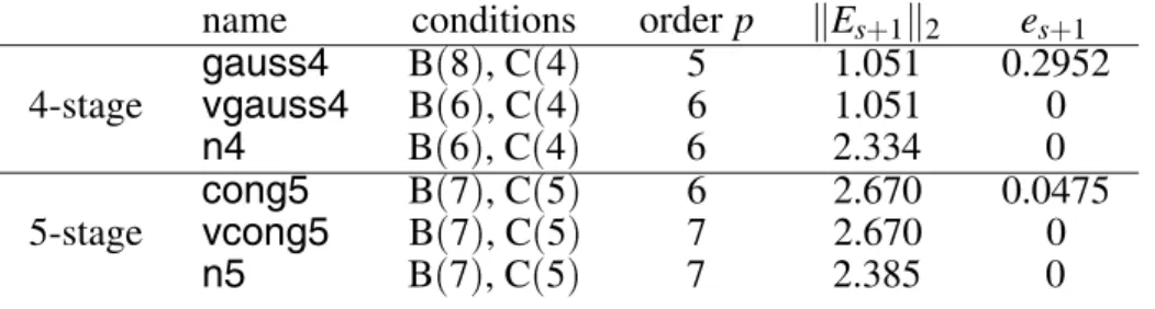
name conditions orderp kEs
+1
k2 es
+1
gauss4 B(8), C(4) 5 1.051 0.2952
4-stage vgauss4 B(6), C(4) 6 1.051 0
n4 B(6), C(4) 6 2.334 0
cong5 B(7), C(5) 6 2.670 0.0475
5-stage vcong5 B(7), C(5) 7 2.670 0
n5 B(7), C(5) 7 2.385 0
Table 1.EPTRK methods
3. Numerical Illustration of the Order Results
To discuss the impact of condition(5) for
EP-TRK methods we construct different sets of co-efficients with 4- and 5-stages and apply the resulting methods to three(non stiff)test
prob-lems.
Construction of 4-stage Methods
We start withs = 4 stages. For any choice of
knotscia method withv =0 is uniquely
deter-mined byB(4)andC(4). The remaining 4
de-grees of freedom can be used to satisfyB(8)with
c-vector taken as Gaussian collocation points, as done for methodgauss4 in Table 1. Here, Es+1 :
= A(c;1)
s
;c
s+1
=(s+1)denotes the
local stage error and es+1 :
= (b
T
+ v
T )Es
+1
denotes the residual of condition(5) in
Theo-rem 2.1. Sincees+1does not vanish, the global
convergence order is only 5.
Global order 6 can be achieved by satisfying C(s),B(s+2)and(5)for givencby computing
vor forv=0 by a special choice ofc. To attain
global order 6 with the same pointsciwe choose v as a solution ofes+1
= 0. But B(6)depends
onvand has to be satisfied, too. With the help of Maple V we calculated a solution
v =0:0 ;0:006332901980013884
;0:319483842974888
0:06964740132900621]:
for this methodvgauss4, see Table 1.
Although it is natural to guarantee condition(5)
for arbitrarily chosen knotsciby introducing a
suitablevvector, it is not necessary. By choos-ing special pointscone can find EPTRK meth-ods withv = 0 which satisfy (5),B(s+2)as
we did for the methodn4with
c=0:1493506562434243
0:6535456428480576 1:123
1:6391116441727] :
Construction of5-stage Methods
The methodcong5was proposed in3]. Due to
small error coefficients, this method performs well for non stiff problems. Sincees+1
6=0 the
global order is p = 6 only, see Table 1. The
methodcong5has the knots
c=0:08858795951270395
0:4094668644407347
0:7876594617608471 1
1:409466864440735] : (6)
With the choicev=0 0 0 0
;0:01842446247125309]and the c-vector (6)
the method vcong5 fulfills(5), B(s+2) and
has global orderp=7.
The methodn5has been constructed withv =0
and
c=0:1365941578442505 0:625
1:230436842527931 1:5
1:6911642569218] :
These values guarantee(5)andB(s+2)and give
a small leading stage error coefficientkEs +1
k.
Test Problems
-12 -10 -8 -6 -4 -2
100 1000
log(Err)
number of steps "gauss4" "vgauss4" "n4"
-12 -10 -8 -6 -4 -2
100 1000
log(Err)
number of steps "cong5" "vcong5" "n5"
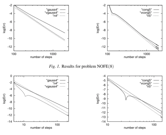
Fig. 1.Results for problem NOFE(8)
-14 -12 -10 -8 -6 -4 -2 0
10 100
log(Err)
number of steps "gauss4"
"n4" "vgauss4"
-14 -13 -12 -11 -10 -9 -8 -7 -6 -5 -4
10 100
log(Err)
number of steps "cong5" "vcong5" "n5"
Fig. 2.Results for problem PROTH(9)
NOFE – a nonlinear problem proposed by
Fehlberg4].
y0
1=2ty1log(max(y2 0:001)) (8a)
y0
2=;2ty2log(max(y1 0:001)) (8b)
t20 5] (8c)
with initial values taken from the exact solution y1(t) = exp(sin(t
2
)) y2(t) =
exp(cos(t
2
)).
PROTH – a(non stiff)Prothero-Robinson
problem, see7].
y0
=λ(y;sin(t))+cos(t)
t 20 10] λ =0:1 (9)
with exact solutiony(t)=sin(t).
ORBIT – a two-body orbit problem, see6].
y0
1=y3 y 0
2=y4 (10a)
y0
3=;
y1 r3 y
0
4=;
y2
r3 t2 0 10] (10b)
r = q
y2 1+y
2
2, with exact solutiony(t) =
cos(t) sin(t) ;sin(t) cos(t)].
We implemented the EPTRK methods of Ta-ble 1 in FORTRAN using douTa-ble precision and applied them to the test problems. (The
code for the method cong5 can be obtained from our web site http://
www.mathematik.uni-halle.de/institute/numerik/software.)
In the figures below we have plotted the number of steps versus the errorERRin the endpoint of the integration, defined by
ERR= v u u t
1 n
n X
i=1
yi;yi(tend)
1+jyi(tend)j
2
:
Notice, fromERR Ch
p follows log
(ERR)
log(C);p log(h
;1
) and therefore the order
of an EPTRK method can be estimated by the slope of the lines in the figures.
The order 6 of the 4-stage methods n4 and
vgauss4 compared with the order 5 of the methodgauss4 leads to a better accuracy for all step sizes. Due to smaller error constants in the step formula(3b)(not shown in Table 1)the
methodn4 withv =0 performs slightly better
-12 -10 -8 -6 -4 -2
100 1000
log(Err)
number of steps "gauss4" "vgauss4" "n4"
-12 -10 -8 -6 -4 -2
100 1000
log(Err)
number of steps "cong5" "vcong5" "n5"
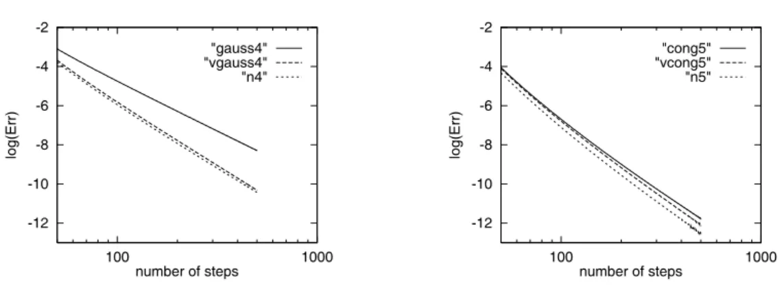
Fig. 3.Results for problem ORBIT(10)
The fact that cong5 is of order 6 only can be seen for sufficient small step sizes, i.e. the slope of the lines in the figures is smaller than the slopes of the (nearly parallel)lines of vcong5
andn5. The best overall performance gives the methodn5withv=0 and small error constants.
4. Stability
The stability of EPTRK methods with v = 0
has been investigated in 10]. The adaption of
the concepts there to the casev 6=0 is
straight-forward. Here, we start with a short review of the notations:
We apply the EPTRK methods to the linear test equation y0
= λy Reλ 0 with constant
step sizeh. Then the solution fulfills the recur-sion
(Ym ym
+1 )
T
=M(z)(Ym
;1 ym
)
T z
=hλ
(11)
with the amplification matrix
M(z)=
zA 1l
z2bTA
+zv
T 1
+zb
T1l
: (12)
We define the stability regionS of an EPTRK
method by
S
:=fz:%(M(z))1g
and have%(M(z)) < 1 ifz is an inner point of
Sand hence
(Ym ym
+1
)!0 form! 1. We
obtain %(M(z))by computing the zeros of the
stability polynomial%(x z):=det(xI;M(z)).
But surprisingly, the new parameters v do not give us any new degree of freedom in the cor-responding stability polynomial. We have the following theorem:
Theorem 4.1. For every method (3) with C(s;
1)and B(s)there exists a corresponding method
with vT =0, satisfying C(s;1), B(s)and
hav-ing the same stability polynomial.
Proof.The rather lengthy proof requires a care-ful study of the stability polynomial. It is given in11].
A consequence of Theorem 4.1 is that it is not possible to improve the stability of EPTRK methods with a choice v 6= 0 for high order
methods. However, a nontrivial choice of the v-vector may be useful to conserve the stability for variable step sizes.
5. Conclusion
We have proposed a superconvergence condi-tion(5)in Theorem 2.1, which allows the
con-struction ofs-stage EPTRK methods with stage order s and convergence order s+2. To
sat-isfy this condition with a given set of knotsci
we have introduced new parameters v into the integration scheme(3). Numerical tests with
fixed step size and 4- and 5-stage methods have illustrated the convergence result. Though it has been possible to find special knotsciwhich
guarantee condition (5) for constant step size
withv=0, for variable step sizes we are forced
to choosev 6=0. Equation(5)becomes
bTm cs
+1
s+1 σs+1
m ;σmA(σm)(c;1) s
+v
T
m c
s+1
s+1 ;
1
σm;1
A(σm
;1
)(c;1) s
with step size ratios σm := hm=hm
;1and σm
-dependent RK matrixA=A(σm)and condition
(5)cannot longer be satisfied withv=0. Since
withv 6= 0 the error behavior is smoother, we
hope to obtain a more reliable error estimation and step size control in this case. This general-ization to variable step sizes will be a topic of further work.
In Theorem 4.1 we have shown that it is not possible to enlarge the stability regions of the EPTRK methods withB(s) and C(s;1) with
the new parametersvof the integration scheme. However, the construction in10]of a EPTRK
method based on a given stability polynomial can be simplified withv6=0.
References
1] Z. BARTOSZEWSKI ANDZ. JACKIEWICZ,
Construc-tion of two-step Runge-Kutta methods of high order for ordinary differential equations, Numerical Al-gorithms18(1998), 51–71.
2] N.H. CONG, A general family of pseudo two-step
Runge-Kutta methods, submitted for publication, 1997.
3] N.H. CONG, H. PODHAISKY,ANDR. WEINER,
Nu-merical experiments with some explicit pseudo two-step RK methods on a shared memory computer, Computers & Mathematics with Applications 36
(1998), 107–116.
4] E. FEHLBERG,Klassische Runge-Kutta Formeln 5.
und 7. Ordnung mit Schrittweitenkontrolle, Com-puting4(1969), 61–71.
5] J.G. FEI,A class of parallel explicit Runge-Kutta
for-mulas, Chinese Journal of Numerical Mathematics and Applications(1994), 23–36.
6] E. HAIRER, S.P. NØRSETT,ANDG. WANNER,Solving
Ordinary Differential Equations I, Springer, 1993.
7] E. HAIRER ANDG. WANNER,Solving Ordinary
Dif-ferential Equations II, Springer, 1996.
8] Z. JACKIEWICZ ANDS. TRACOGNA,A General Class
of Two-Step Runge-Kutta Methods for Ordinary Differential Equations, SIAM J. Numer. Anal. 32
(1995), 1390–1427.
9] H. PODHAISKY, Parallele explizite Zweischritt
Runge-Kutta-Methoden, Diplom-Thesis, Univer-sit¨at Halle, 1998.
10] H. PODHAISKY ANDR. WEINER,A Class of Explicit
Two-Step Runge-Kutta Methods with Enlarged Sta-bility Regions for Parallel Computers, Parallel Com-putation(P. Zinterhofer, M. Vajterˇsic, and Andreas
Uhl, eds.), Lecture Notes in Computer Science,
1557, Springer, 1999, pp. 68–77.
11] H. PODHAISKY, R. WEINER,ANDJ. WENSCH,High
Order Explicit Two-Step Runge-Kutta Methods for Parallel Computers, Tech. Report 19, Universit¨at Halle, FB Mathematik/Informatik, 1999.
Received: May 15, 1999
Accepted in revised form:January 21, 2000
Contact address:
H. Podhaisky, R. Weiner and J. Wensch Fachbereich Mathematik unf Informatik Institut f¨ur Numerische Mathematik Martin–Luther–Universit¨at Halle-Wittenberg Theodor-Lieser-Straße 5 D-06120 Halle Germany e-mail:
fpodhaisky,weiner,[email protected]
HELMUT PODHAISKYreceived his diploma in mathematics from the University of Halle, Germany and is currently a doctoral candidate at the same Department.
R¨UDIGERWEINERis Full Professor of Scientific Computing at the
Uni-versity of Halle. He received his diploma in mathematics in 1977 from the University in Kharkov(Ukraina)and his Ph.D from the University of Halle.