Winter 2015
EPQ model with scrap and backordering under Vendor
managed inventory policy
Maryam Akbarzadeh1, Maryam Esmaeili1*, Ata Allah Taleizadeh2 1
Department of Industrial Engineering, Alzahra University, Tehran, Iran m.akbarzadeh66@yahoo.com, esmaeili_m@alzahra.ac.ir
2
School of Industrial Engineering, College of Engineering, University of Tehran, Tehran, Iran taleizadeh@ut.ac.ir
Abstract
This paper presents the economic production quantity (EPQ) models for the imperfect quality items produced with/without the presence of shortage condition. The models are presented in a two-level supply chain composed of a single manufacturer and a single buyer to investigate the performance of vendor-managed inventory (VMI) policy. The total costs are minimized to obtain the optimal production lot size and the allowable backorder level before and after applying VMI policy. Numerical examples and sensitivity analysis based on certain parameters are performed to show the capability of the proposed supply chain model enhanced with VMI policy.
Keywords: Economic production quantity (EPQ), Vendor-managed inventory (VMI), Supply chain, Defective items
1.
Introduction and literature review
Economic Production Quantity (EPQ) has been applied widely in the manufacturing sector to optimize the production quantity or lot-sizing considering the capacities and limitations. Although, all EPQ models minimize the total costs or maximize the manufacturer’s profit apparently, they are different mainly regarding various assumptions. One of the impractical assumptions of the EPQ models is that all units have perfect quality. However, in practice, most of the manufacturing processes are not free of defect and cause non-conforming items. Generally, these non-conforming items are categorized into two groups: the repairable and the scrap (the latter is discarded).
1*
Corresponding Author
Recent developments in information technology have facilitated the advent of new supply chain initiatives such as vendor managed inventory (VMI) policy. VMI is a supply chain initiative where the vendor decides on the appropriate inventory levels of each of the products and the appropriate inventory policies to sustain those levels. It is also known as continuous replenishment or supplier-managed inventory. VMI becomes more critical for the EPQ models with imperfect quality production. In this paper, the EPQ model based on VMI policy is considered for the defective items produced under the presence and absence of the shortage. The models are developed for a two-level supply chain consisting of a single manufacturer and a single buyer and examine the inventory management practices before and after implementing VMI. Therefore, the literature reviews are organized for both EPQ models with scrap and VMI policy.
Many researchers introduced EPQ models with scrap such as Salameh and Jaber (2000). They developed an inventory model which explained imperfect quality items using the EPQ/EOQ formulates. They supposed that the defective items are sold as a single batch at the end of the total screening process. Cardenas-Barron (2000) also revised Salameh and Jaber's (2000) model and showed that the error only affects the optimal order size value. Later, Goyal and Cardenas-Barron (2002) developed Salameh and Jaber's (2000) model and proposed a practical approach to determine EPQ for imperfect quality items. Goyal et al. (2003) studied the model of Goyal and Cardenas-Barron (2002), regarding vendor-buyer integration. Konstantaras et al. (2007) presented a production-inventory model for defective items regarding two conditions. The first one was to sell the items to a secondary shop as a single batch at a lower price comparing to new ones and the second one was to rework them at some cost and return to its original quality. Wee et al. (2007) and Eroglu and Ozdemir (2007) extended the model of Salameh and Jaber (2000) independently regarding the shortages permit. Cardenas-Barron (2008) proposed a simple derivation to find an optimal manufacturing batch size with rework process in a single stage production system. Khan et al. (2011) extended the Salameh and Jaber (2000) EOQ model for imperfect items and presented a detailed review of EOQ/EPQ models with imperfect quality. Recently, Hsu and Hsu (2013) built two optimal production quantity models with imperfect production processes, inspection errors, planned backorders, and sales returns. Taheri-Tolgari et al. (2012) presented a discounted cash-flow approach for an inventory model for imperfect items under inflationary conditions with considering inspection errors and related defect sales return issues. Sarkar and Moon (2011) developed a production inventory model in an imperfect production system considering stochastic demand and the effect of inflation. Pal et al. (2013) derived a mathematical model on EPQ with stochastic demand in an imperfect production system. Cárdenas-Barrón et al. (2012) derived jointly both the optimal replenishment lot size and the optimal number of shipments for the inventory models.
The success of a firm will depend on its ability to integrate with other participants in the chain responsible for physical, financial and information flows. Organizations are striving to achieve joint total effectiveness across the entire chain. This has given rise to a need for various coordination mechanisms. Vendor Managed Inventory (VMI) is one of the practices which has gained a lot of attention in recent times. Many companies such as HP, Shell and Walmart have reportedly adopted VMI. Researchers are actively engaged in studying issues related to VMI, including, but not limited to, replenishment decisions, contracts, relationships as well as the strategic implications of such a mechanism (Marques et al., 2010). The costs of VMI policy with the traditional one are highly compared in the literature (Waller et al. (1999),
Cetinkaya and Lee (2000)). Moreover, having a deterministic demand is one of the usual assumptions (Valentini and Zavanella (2003), Shah and Goh (2006), Woo et al. (2001)). They considered a supply chain consisting of a single manufacturer and multiple buyers or retailers. Kleywegt et al. (2002) presented an inventory routing problem of a manufacturer who owns the inventory at the retailers. An approximation method is used to find the minimum-cost routing policy. Later Zhang et al. (2007) extended Woo et al.’s model by omitting the common replenishment cycle assumption and having different ordering cycles for the retailers. A number of papers analyzed the VMI policy in a supply chain as a centralized or a coordination channel. For instance, Bernstein et al. (2006) studied the constant wholesale price and quantity discount contracts. They showed the role of VMI in a complete coordination in a supply chain with multiple competing retailers. It is shown that the performance of the overall system is improved in VMI regarding certain conditions (Nagarajan and Rajagopalan (2008)). Pasandideh et al. (2010) considered the retailer-supplier partnership through a VMI. In addition, they developed an economic order quantity (EOQ) with shortage to explore the effects of important supply chain parameters on the cost savings realized from VMI. Ma et al. (2013) developed a VMI model for a supply chain with one vendor and one retailer including a VMI warehouse near the retailer and with a freshness clause. They showed that the freshness clause had a significant impact on the decisions of both vendor and retailer. Hariga et al. (2013a&b) analyzed a VMI system with different replenishment cycles for different retailers. Kannan et al. (2013) studied the benefits of a VMI arrangement when the same organization owns the vendor and the retailers. Some of these studies, like Darwish and Odah (2010) and Kannan (2013), also showed that adopting VMI leads to system wide cost reductions.
Regarding the effectiveness of VMI, we studied the integration of VMI policy in EPQ models producing defective items in this paper. To the best our knowledge, it has been ignored in the literature. Therefore, in this paper, we present the EPQ model to investigate the performance of VMI in a two-level supply chain composed of a manufacturer and a buyer. The manufacturer produces defective items under the presence and absence of the shortage costs. The production process generates randomly imperfect quality items at a constant production rate. The manufacturer and the buyer are faced with the setup cost, production cost, screening cost, disposal cost per scrap item, holding cost and ordering cost without shortage. The optimal production lot size is obtained by minimizing the total expected inventory costs before and after implementing VMI. The backordering cost per item per time unit is also considered regarding shortage permission in addition to the costs mentioned. The total expected inventory costs are minimized to obtain the optimal maximum allowable backorder level and production lot size before and after implementing VMI. The numerical example is presented in this paper, including sensitivity analysis of certain parameters. It shows the capability of supply chain regarding implementing VMI with and without shortage. Although a simple supply chain is used for computational ease, the obtained results can be generalized to more complex supply chains.
The rest of this paper is organized as follows. Section 2 reviews the notation and problem formulation. Section 3 presents the model formulations. In Section 4, the numerical example and the sensitivity analysis are presented to analyze the effect of different parameters on the optimal economic production quantity and the total cost before and after implementing VMI. The final section is dedicated to conclusions and recommendations for future studies.
2.
Notation and problem formulation
This section introduces the notation and formulation used in the models. Specifically, all decision variables, input parameters and assumptions underlying the models will be stated. 2.1. Input parameters
The following notations are used in the paper: Q: The production lot size
QVMI: The production lot size in VMI
B: The maximum allowable backorder level
BVMI: The maximum allowable backorder level in VMI
P: The production rate
λ: The demand rate
x: The defective rate, a random variable with known probability density function d: The production rate of defective items (during the regular production
process), in units per time unit
H: The maximum level of on-hand inventory in units, when the rework process ends
b: The backordering cost per item per time unit K : The manufacturer setup cost
K : The buyer ordering cost
C: The production cost (screening cost for each item is included)
C : The repair cost of each imperfect quality item reworked (screening cost for each rework item is also included)
C : The disposal cost per scrap item, h: The holding cost
TC(Q): The total cost per time unit
E(TCU ): The manufacturer’s expected total cost before VMI in case i (i=1,2) E(TCU ): The buyer’s expected total cost before VMI in case i
E(TCU ): The manufacturer’s expected total cost in VMI in case i E(TCU ): The buyer’s expected total cost in VMI in case i
E(TCU ): The expected total cost before VMI in case i E(TCU ): The expected total cost of VMI in case i
2.2. Assumptions
The mathematical models are developed based on the following assumptions.
(a) A single-manufacturer-single-buyer supply chain with defective items is considered. (b) The production rate P is a constant and is greater than the demand rate λ.
(c) The EPQ model is imperfect and production process generates randomly x percent of imperfect quality items at production rate d.
3.
Model formulations
The models are presented in two cases; 1: shortage is not allowed, 2: shortage is allowed and is completely backordered.
3.1. Case 1. Shortage is not permitted
The model with the random defective rate and an imperfect rework process without shortage is depicted in Figure 1. According to assumption b, P is greater than or equal to the sum of the
demand rate λ and also P d 0 or0 x 1 P
. Therefore, based on Figure (1), the
production cycle length (T) is
1 2
1
Q x
T t t
(1)
Since t1 Q H
P P d
1 (1 )
H P d t Q x
P
(2)
The total defective items produced during the regular production uptime “t1” are:
1
dt
xQ
(3)The production downtime time “t2” needed for consuming the maximum on-hand inventory H
is computed in Eq. (4).
2
1 1
H x
t Q
P
(4)
3.1.1. Supply chain without VMI policy
Regardless of implementing VMI, the inventory cost of the manufacturer, the buyer and the total inventory cost of the supply chain are as follows:
01 ( ) 1 2 1
2 2
m S m
H x Q
T C Q CQ C x Q K h t t h t
(5)
01
b b
T C K (6)
( )
1 2
12 2
S m b
H xQ
TC Q CQC xQ K h t t h t K
(7)
The proportion of defective items x is considered to be a random variable with a known probability density function. Thus, the expected value of x is used in the inventory cost analysis. Since the production cycle length is not a constant, by using the renewal theorem approach (Zipkin, 2000) we have;
E T C Q E T CU Q
E T
(8)
Where,
Q
1
E T E x
(9)
Then,
01 2 1 1 11 1 1 2 1
1
1 2 1
S m
m
C E x K
C h
E T CU Q
E x E x Q E x P E x
E x
E x hQ
hQ
P E x E x
(10) And also,
01 1 1 b b KE TCU Q
Q E x
(11)
If we let
0 1 , 1 E E x
1 1 E x E E x and
2 2 1 E x E E x
for some simplifications we
have:
01 0 1 0
0 1 2
. . .
1 . . 1
2 2
m
m S
K
E TCU Q C E C E E
Q
hQ hQ
E h Q E E
P P (12)
01 . 0
b b
K
E TCU Q E
Q
01 0 1 0
0 1 2
( ) 1 1 2 2 m b S K K
E TCU Q CE C E E
Q
hQ hQ
E hQ E E
P P (14)
Since the second derivative of E TCU 01
Q respect to Q is positive,2Km3 E0 0Q
, the total objective cost is convex. Then the optimal production quantity is obtained by setting the first
derivative of
01 m
E TCU Q respect to Q equal to zero yielding;
*2
2
1 2 1 .
m
K Q
h h E x h E x
P P (15)
3.1.2. Supply chain with VMI policy
After implementing VMI, the total cost of the buyer, the manufacturer and the chain are calculated as below;
11 ( ) 1 2 1
2 2
VMI
m VMI V MI S VMI m b
xQ H
TC Q CQ C xQ K h t t h t K
(16)
11
0
b
TC
(17)
11 11
1 2 1
( )
2 2
V MI V MI m V MI b V MI
V MI
V MI S V MI m b
TC Q T C Q T C Q
xQ H
CQ C xQ K h t t h t K
(18)
Using
E
0,
E
1,E
2defined in the previous section, we have,
11 0 1 0 0
1 2 ( ) 1 2 1 2
m b VMI
m VMI S
VMI
VMI VMI
K K hQ
E TCU Q CE C E E E
Q P
hQ
hQ E E
P (19) 11 0 b
E T CU (20)
11 11
11
0 1 0 0
1 2 ( ) 1 2 1 2
V MI m V MI b V MI
m b V MI
S
V MI
V MI V MI
E TCU Q E TCU Q E T CU Q
K K hQ
CE C E E E
Q P
hQ
hQ E E
P (21)
Since the second derivative of E TCU Q 11
VMI
respect to QVMIis positive,
0 3
2
0
m b
VMI
K K
E Q
,
the total objective cost is convex. Then the optimal production quantity is obtained by setting the first derivative ofE TCU m01QVMI respect to QVMIequal to zero yielding;
*
2
2
1 2 1 .
m b
VMI
K K
Q
h h E x h E x
P P
(22)
3.2. Case 2 .Shortage is permitted
The inventory control in this case is shown in Figure 2. According to the definitions in case
1, we have:
1
H t
P d
(23)
2
H t
(24)
3
B t
(25)
4
B t
P d
(26)
Q
H P d B
P
(27)
1 4
Q
t t
P
(28)
The cycle length T is:
4 1 1 i i x Q T t
(29)3.2.1. Supply chain without VMI policy
In this case, the inventory cost of the manufacturer, the buyer and the total inventory costs of the chain are as below;
02
1 4
1 2 3 4 1 4
, . .
2 2 2
m S m
d t t
H B
TC Q B CQC x QK h t t b t t h t t
(30)
02
b b
T C K (31)
1 4
1 2 1 4 3 4
, ( )
2 2 2
noVMI S m b
d t t
H bB
TC Q B C C x QK h t t t t t t K
(32)
Similar to the first case, by using the renewal theorem approach (Zipkin, 2000), we have:
02 2 2 1 1, 1 2
1 1 2 1
1
1
2 1 1 2 1
1
S m
m
C C E x K h
E TCU Q B Q B
E x Q E x P E x
E x
b h E x
B x hQ
E h B Q
Q E x P E x E x
x P (33) And also:
02 1 . 1 b b KE TCU Q
Q E x
(34)
By considering
0 1 , 1 E E x
1 1 E x E E x ,
2 2 1 E x E E x and
3 1 1 1 1 x E E E x x P
02 0 1 0 0
2
3 1 2
, 1 2
2 1 2 2 m m S K h
E TCU Q B CE C E E Q B E
Q P
B hQ
b h E h B Q E E
Q P (35)
02 0 b b KE TCU Q E
Q
(36)
Therefore, the total expected inventory costs are,
02 0 1 0 0
2
3 1 2
( )
, 1 2
2
1
2 2
m b
S
K K h
E T CU Q B CE C E E Q B E
Q P
B hQ
b h E h B Q E E
Q P (37)
To prove the convexity of
02 ,
m
E TCU Q B with respect to Q and B, the Hessian matrix is
utilized (Rardin, 1998). Therefore:
02 02 02 02 2 2 0 2 2 2 2 , , 2 0 , , m m m m mE TCU Q B E TCU Q B
Q
Q Q B K
Q B E
B Q
E TCU Q B E TCU Q B
B Q B
(38)Since (38) is strictly positive, equating the first derivative of
02 ,
m
E TCU Q B with respect
to Q and B to zero yields the optimal values as below.
* 1 2 2 2 2 11 1 2 1
1
m
K
h x
h E x E h E x hE x
P b h x P
P
Q
(39)
1* 1 *
1
1
B h Q
b h
x
E x E
x P (40)
3.2.2. Supply chain with VMI policy
After implementing VMI, the total cost of the buyer, the manufacturer and the chain are calculated as below;
12 1 2 3 4
1 4 1 4 , 2 2 2 V MI
m V M I V MI V MI S V MI m
b
B H
TC Q B CQ C xQ K h t t b t t
d t t
h t t K
(41) 12 0 b
T C (42)
1 2 3 4
1 4 1 4 , 2 2 2 V MI
V MI V MI V MI V MI S V MI m
b
B H
TC Q B CQ C xQ K h t t b t t
d t t
h t t K
(43)
For some simplifications,
2 2 1 E x E E x
and 3
1 1 1 1 x E E E x x P ,and then:
12 20 0 2
2
3 1 0 1
( )
, 1 2
2 2
1 2
m b VMI
m V MI V MI V MI V MI
V MI V MI
VMI V MI S
V MI
K K h hQ
E TCU Q B E Q B E E
Q P
B
b h E h B Q E CE C E
Q P (44) 12 0 b
E T CU
(45)
12 12 120 1 0 0
2 2
3 1 2
, , ( ) 1 2 2 1 2 2
V MI V MI m V MI VMI b
m b
S VMI V MI
VMI
VMI V MI
VMI VMI
VMI
E TCU Q B E TCU Q B E TCU
K K h
CE C E E Q B E
P Q
B hQ
b h E h B Q E E
P Q (46)
To prove the convexity ofE TCU 12
QV MI,BV M I
with respect toQ
VMI andB
VMI the Hessian
2 2 12 12 2 2 12 12 2 2 0 , , , , 2 0 VMI VMI VMI VMI VMI VMIVMI VMI VMI VMI VMI VMI
VMI
VMI VMI
VMI VMI VMI
m b VMI
E TCU Q B E TCU Q B
Q Q B Q
Q B
B
E TCU Q B E TCU Q B
B Q B
K K E Q
(47)Since the result is strictly positive, equating the first derivative ofE TCU
12
QVMI,BVMI
with respect to
Q
VMI andB
VMI to zero yields the optimal values as below.
* 1 2 2 2 2 11 1 2 1
1 m b VMI K K Q h x
h E x E h E x hE x
P b h P
x P (48) 1
*
1
*1
VMI VMI
h
b h
x
B
E
Q
x
P
(49)4.
Numerical example and sensitivity analysis
Consider a manufacturer who produces aluminum doors in different sizes. Because of the especial manufacturing process and according to the different types of orders, both machine and laborers have important roles in the production process. So, producing doors in different sizes without defective is inevitable, but using rework process, this problem can be removed from the products. Also, because of humans’ errors which are different in all laborers, the defective production rate is a stochastic variable during the production process and depends on the experiments of laborers. In addition, because of specifications of products the items are produced according to a contract and are held by the manufacturer which means vendor managed inventory is being used by the manufacturer.
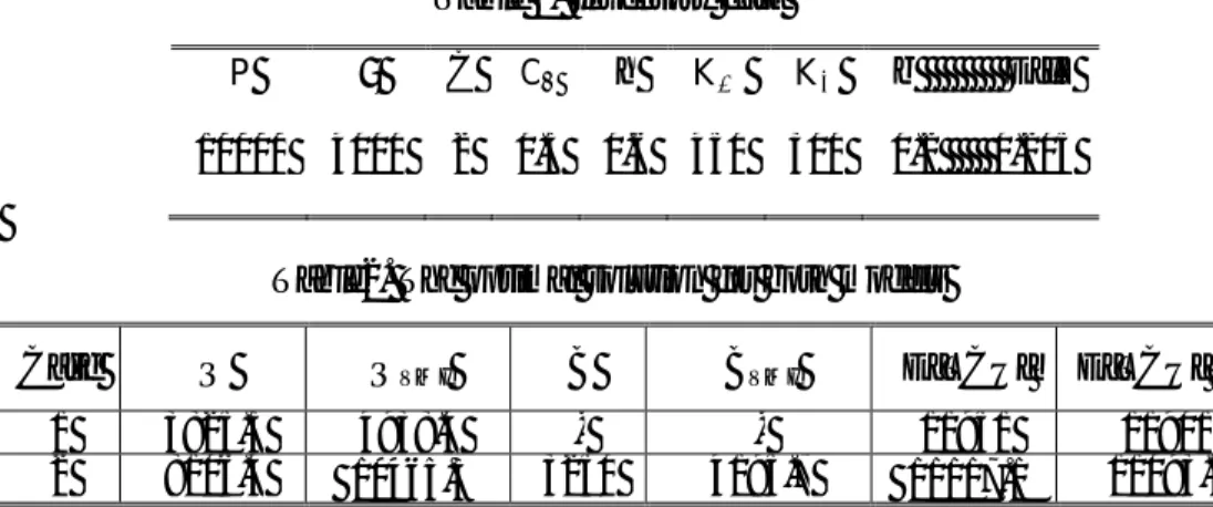
Assume that the demand rate of products is 4,000 units per year. Items are produced at a rate of 10,000 units per year. The financial department has estimated that it costs 450$ to initiate a production run, each unit costs the company 2$ to manufacture, the holding cost is 0.6$ per item per year, and the disposal cost is 0.3$ for each scrap item. The production rate of defective items is uniformly distributed over the interval [0, 0.41]. The inventory data are shown in Table 1 and the optimal solutions for both models are shown in Table 2.
Table 1. Inventory data
Table2. The optimal solution for both models
Case Q QVMI B BVMI E[TCU] E[TCU] VMI
1 3825.3 4938.4 - - 11951 11901 2 8106.4 10465.3 3250 4195.7 11117.1 11093.5
To consider the effect of parameters on the optimal solution in both models, sensitivity analysis is performed in this paper. At each stage, one parameter is changed by +75%, +50%, +25%, -25%, -50% and -75% and the rest of the parameters remain at their original levels. The results are shown in Tables 3 and 4.
Table 3. The effect of changes of certain parameters on the optimal solution in the first model (without shortage)
Parameter
%Changes Q QVMI E[TCU] E[TCU] VMI
C
-75 3825.300 4,938.400 4403.500 4353.400 -50 3825.300 4,938.400 6919.200 6869.100 -25 3825.300 4,938.400 9435.000 9384.900 +25 3825.300 4,938.400 14466.000 14416.000 +50 3825.300 4,938.400 16982.000 16932.000 +75 3825.300 4,938.400 19498.000 19448.000
s
C
-75 3825.3 4,938.4 11719 11668 -50 3825.3 4,938.4 11796 11746 -25 3825.3 4,938.4 11873 11823 +25 3825.3 4,938.4 11719 11978 +50 3825.3 4,938.4 11796 12055 +75 3825.3 4,938.4 11873 12133
h
-75 7650.6 9,876.9 11626 11601 -50 5409.8 6,984 11953 11917 -25 4417.1 5,702.4 12203 12160 +25 3421.5 4,417.1 12601 12545 +50 3123.3 4,032.2 12770 12708 +75 2891.7 3,733.1 12924 12858
m
K
-75 1912.7 3,662.5 11753 11506 -50 2704.9 4,131.8 11767 11651 -25 3312.8 4,553 11853 11781 +25 4276.8 5,295.9 12049 12011 +50 4685 5,630.7 12144 12115 +75 5060.4 5,946.7 12237 12213
P λ C C h K K b E[x] 10000 4000 2 0.3 0.6 450 300 0.2 0.205
Table 3. Continue Parameter
%Changes Q QVMI E[TCU] E[TCU] VMI
b
K
-75 3825.3 4,131.8 12119 12115 -50 3825.3 4,417.1 12218 12203 -25 3825.3 4,685 12316 12286 +25 3825.3 5,179.5 12513 12439 +50 3825.3 5,409.8 12612 12511 +75 3825.3 5,630.7 12711 12579
E x is increasing cumulatively at the rate of 0.05 in the interval [0.005,0.5]
E x
0.05 3178.100 4,102.900 9564.100 9515.900 0.055 3339.400 4,311.200 10056.000 10008.000 0.105 3503.900 4,523.500 10610.000 10561.000 0.155 3667.700 4,735.000 11236.000 11187.000 0.205 3825.300 4,938.400 11951.000 11901.000 0.255 3969.900 5,125.200 12772.000 12720.000 0.305 4093.700 5,284.900 13725.000 13671.000 0.355 4188.300 5,407.100 14840.000 14784.000 0.405 4246.700 5,482.400 16162.000 16102.000 0.455 4263.800 5,504.500 17746.000 17681.000
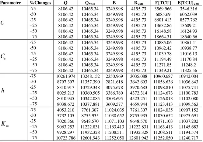
Table 4. The effect of changes of certain parameters on the optimal solution in the second model (with shortage)
Parameter %Changes Q QVMI B BVMI E[TCU] E[TCU]VMI
C
-75 8106.42 10465.34 3249.998 4195.73 3569.966 3546.316 -50 8106.42 10465.34 3249.998 4195.73 6085.69 6062.039 -25 8106.42 10465.34 3249.998 4195.73 8601.413 8577.762 +25 8106.42 10465.34 3249.998 4195.73 13632.86 13609.21 +50 8106.42 10465.34 3249.998 4195.73 16148.58 16124.93 +75 8106.42 10465.34 3249.998 4195.73 18664.31 18640.66
s
C
-75 8106.42 10465.34 3249.998 4195.73 10885.06 10861.41 -50 8106.42 10465.34 3249.998 4195.73 10962.42 10938.77 -25 8106.42 10465.34 3249.998 4195.73 11039.78 11016.13 +25 8106.42 10465.34 3249.998 4195.73 11194.49 11170.84 +50 8106.42 10465.34 3249.998 4195.73 11271.85 11248.2 +75 8106.42 10465.34 3249.998 4195.73 11349.21 11325.56
h
-75 10261.974 13248.152 2350.969 3035.088 10960.687 10942.004 -50 8797.397 11357.390 2821.618 3642.693 11058.636 11036.843 -25 8310.917 10729.348 3075.678 3970.683 11098.810 11075.741 +25 8025.213 10360.505 3386.780 4372.314 11124.673 11100.783 +50 8010.945 10342.085 3503.695 4523.251 11126.013 11102.080 +75 8038.672 10377.881 3609.577 4659.944 11123.413 11099.563
m
K
-75 4053.210 7761.307 11024.035 7761.307 11024.035 10907.152 -50 5732.105 8755.935 11030.652 8755.935 11030.652 10975.691 -25 7020.366 9648.570 11071.103 9648.570 11071.103 11037.202 +25 9063.253 11222.831 11163.413 11222.831 11163.413 11145.683 +50 9928.297 11932.328 11208.511 11932.328 11208.511 11194.574 +75 10723.786 12601.943 11252.050 12601.943 11252.050 11240.717
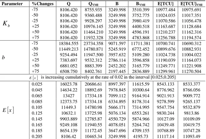
Table 4. continue
Parameter %Changes Q QVMI B BVMI E[TCU] E[TCU]VMI
b
K
-75 8106.420 8755.935 3249.998 3510.399 10977.484 10975.691 -50 8106.420 9360.488 3249.998 3752.775 11024.035 11017.351 -25 8106.420 9928.297 3249.998 3980.419 11070.586 11056.478 +25 8106.420 10976.145 3249.998 4400.518 11163.687 11128.684 +50 8106.420 11464.210 3249.998 4596.191 11210.237 11162.316 +75 8106.420 11932.328 3249.998 4783.868 11256.788 11194.574
b
-75 18384.555 23734.358 9071.597 11711.381 10700.741 10690.312 -50 11449.213 14780.871 5245.919 6772.452 10899.676 10882.931 -25 9254.494 11947.500 3957.632 5109.280 11024.738 11004.022 +25 7383.697 9532.312 2786.114 3596.858 11190.039 11164.073 +50 6881.052 8883.399 2452.202 3165.779 11249.771 11221.908 +75 6508.750 8402.761 2197.445 2836.889 11299.961 11270.504
E x is increasing cumulatively at the rate of 0.02 in the interval [0.025,0.205]
E x
0.025 16023.78 20686.61 8997.397 11615.59 8543.133 8533.377 0.045 14634.22 18892.69 7978.845 10300.64 8776.962 8766.056 0.065 13427 17334.18 7099.112 9164.914 9021.913 9009.772 0.085 12373.75 17334.18 6334.895 8178.314 9278.599 9265.137 0.105 11449.3 14780.98 5666.171 7314.995 9547.754 9532.879 0.125 10632.1 13725.98 5076.134 6553.261 9830.244 9813.86 0.145 9903.889 12785.87 4550.729 5874.966 10127.09 10109.09 0.165 9249.108 11940.55 4078.051 5264.742 10439.48 10419.75 0.185 8654.139 11172.45 3647.696 4709.155 10768.89 10747.28 0.205 8106.42 10465.34 3249.998 4195.73 11117.14 11093.49
According to the obtained results from Tables 3 and 4, the following achievements are shown in Table 5.
Table 5. The effects of changing parameters on optimal solutions
P ar a m e te r c h an g e (F r o m -75% to + 75)
Effects of parameter change on optimal solutions
Q QVMI B BVMI E[TCU] E[TCU]VMI
C as e 1 C as e 2 C as e 1 C as e 2 C as e 1 C as e 2 C as e 1 C as e 2 C as e 1 C as e 2 C as e 1 C as e 2
C None None None None - None - None Increas
e Increas e Increas e Increas e
Cs None None None None - None - None
Increas e Increas e Increas e Increas e
h Decrease Decrease Decrease Decrease - Increase - Increase Increas e Increas e Increas e Increas e
Km Increase Increase Increase Increase - Increase - Increase
Increas e Increas e Increas e Increas e
Kb None None None None - None - None
Increas e Increas e Increas e Increas e
b - Decreas
e -
Decreas
e -
Decreas
e -
Decreas
e -
Increas
e -
Increas e
E(x) Decrease Decrease Decrease Decrease - Decreas
e -
Decreas e Increas e Increas e Increas e Increas e
Considering the above mentioned results, VMI policy is more beneficial for both parties in the both models that is to say the expected total cost after implementation of VMI is less than the expected total cost in traditional supply chain. Besides, the optimal production quantity in VMI is greater than its quantity in the traditional policy.
5.
Conclusions and future research
In this paper, the performance of the VMI policy in a two-echelon supply chain consisting of a manufacturer and a buyer is investigated regarding two conditions, with and without shortage. The production process generates randomly imperfect quality items at a constant production rate. The optimal production quantity and backordered level are obtained by minimizing total cost of the supply chain. The numerical example and sensitivity analysis have been performed to illustrate the differences in total cost and an optimal solution of both models. It is demonstrated that the VMI policy is more beneficial for both parties in the both models. Moreover, the optimal production quantity in VMI is greater than its quantity in the traditional policy.
There is much scope in extending the paper. For example, full backordering could consider partial backordering. Also, the levels of supply chain and the number of buyers could increase. In this case, we could investigate the impact of non-cooperative and cooperative relationships between the buyers.
References
Bernstein, F., Chen, F., & Federgruen, A. (2006). Coordinating supply chains with simple pricing schemes: the role of vendor managed inventories. Management Science, 52, 1483–1492.
Cardenas-Barron, L.E. (2000), Observation on: economic production quantity model for items with imperfect quality, [International Journal of Production Economics, 64, 59–64],
International Journal of Production Economics, 67, 201.
Cardenas-Barron, L.E. (2008). Optimal manufacturing batch size with rework in a single-stage production system - a simple derivation. Computers & Industrial Engineering, 55,758–765. Cárdenas-Barrón, L.E., Taleizadeh, A.A., & Trevino-Garza, G. (2012). An improved solution to replenishment lot size problem with discontinuous issuing policy and rework, and the multi-delivery policy into economic production lot size problem with partial rework. Exp Syst Appl, 39,13540–6.
Cetinkaya, S., & Lee, C.Y. (2000). Stock replenishment and shipment scheduling for vendor managed inventory systems. Management Science, 46, 217–232.
Darwish, M. A., & Odah, O. M. (2010). Vendor managed inventory model for single-vendor multi-retailer supply chains. European Journal of Operational Research, 204(3), 473-484.
Eroglu, A., & Ozdemir, G. (2007). An economic order quantity model with defective items and shortages. International Journal of Production Economics, 106,544–549.
Goyal, S.K., & Cardenas-Barron, L.E. (2002). Note on: economic production quantity model for items with imperfect quality - a practical approach. International Journal of Production Economics, 77,85–87.
Goyal, S.K., Huang, C.K., & Chen, H.K. (2003). A simple integrated production policy of an imperfect item for vendor and buyer. Production Planning & Control,14,596–602.
Hariga, M., Gumus, M., & Daghfous, A. (2013a). Storage constrained vendor managed inventory models with unequal shipment frequencies. Omega (Accepted).
Hariga, M., Gumus, M., Daghfous, A., & Goyal, S. K. (2013b). A vendor managed inventory model under contractual storage agreement. Computers & Operations Research, 40(8), 2138-2144.
Hsu, J.-T., & Hsu, L.-F. (2013). Two EPQ models with imperfect production processes, inspection errors, planned backorders, and sales returns. Comput. Ind. Eng, 64 (1), 389–402. Kannan, G., Grigore, M. C., Devika, K., & Senthilkumar, A. (2013). An analysis of the general benefits of a centralised VMI system based on the EOQ model. International Journal of Production Research, 51(1), 172-188.
Khan, M., Jaber, M.Y., Guiffrida, A.L., & Zolfaghari, S. (2011). A review of the extensions of a modified EOQ model for imperfect quality items. Int. J. Prod. Econ., 132 (1), 1–12.
Kleywegt, A.J., Nori, V.S., & Savelsberg, M.W.P. (2002). The stochastic inventory routing problem with direct deliveries. Transportation Science, 36,94–118.
Konstantaras, I., Goyal, S.K., & Papachristos, S. (2007). Economic ordering policy for an item with imperfect quality subject to the in-house inspection. International Journal of Systems Science, 38,473–482.
Ma, S., Ying, D., Guan, X., & Huang, K. (2013). Managing inventory through (Q, r) policy for a VMI programme with freshness clause. International Journal of Applied Management Science, 5(2), 129 – 143.
Marquès, G., Thierry, C., Lamothe, J., & Gourc, D. (2010). A review of Vendor Managed Inventory (VMI): from concept to processes. Production Planning & Control, 21(6), 547-
561.
Nagarajan, M., & Rajagopalan, S. (2008). Contracting under vendor managed inventory systems using holding cost subsidies. Production and Operations Management, 17, 200–210.
Pal, B., Sana, S.S, & Chaudhuri, K.S. (2013). A mathematical model on EPQ for stochastic demand in an imperfect production system. J Manufact Syst, 32, 260–270.
Pasandideh, S.H.R., Akhavan Niaki, S.T., & Roozbeh Nia, A. (2010). An investigation of vendor-managed inventory application in supply chain: the EOQ model with shortage. The International Journal of Advanced Manufacturing Technology , 49, 329–339.
Salameh, M.K., & Jaber, M.Y. (2000). Economic production quantity model for items with imperfect quality. International Journal of Production Economics, 64, 59–64.
Sarkar, B., & Moon, I. (2011). An EPQ model with inflation in an imperfect production system.
Appl. Math. Comput, 217 (13), 6159–6167.
Shah J., & Goh M. (2006). Setting operating policies for supply hubs. International Journal of Production Economics, 100, 239–252.
Taheri-Tolgari, J., Mirzazadeh, A., & Jolai, F. (2012). An inventory model for imperfect items under inflationary conditions with considering inspection errors. Comput. Math. Appl, 63 (6), 1007–1019.
Valentini, G., & Zavanella, L. (2003). The consignment stock of inventories: industrial case and performance analysis. International Journal of Production Economics, 81–82,215–224.
Waller, M., Johnson, M.E. & Davis, T. (1999). Vendor-managed inventory in the retail supply chain. Journal of Business Logistics, 20, 183–203.
Wee, H.M., Yu, J., & Chen, M.C. (2007). Optimal inventory model for items with imperfect quality and shortage backordering. Omega, 35,7–11.
Woo, Y., Hsu, S., & Wu, S. (2001). An integrated inventory model for a single vendor and multiple buyers with ordering cost reduction. International Journal of Production Economics, 73, 203–215.
Zhang, T., Liang L., Yu, Y., & Yu, Y. (2007). An integrated vendor-managed inventory model for a two-echelon system with order cost reduction. International Journal of Production Economics, 109, 241–253.