LABTS: A Learning Automata-Based Task
Scheduling Algorithm in Cloud Computing
Neda Zekrizadeh
Department of Computer Engineering, Science and Research Branch
Islamic Azad University Tehran, Iran [email protected]
Ahmad Khademzadeh
* Iran Telecommunication Research Center (ITRC)Tehran, Iran [email protected]
Mehdi Hosseinzadeh
Health Management and EconomicsResearch Center,
Iran University of Medical Sciences, Tehran, Iran
Received: 17 August 2018 - Accepted: 14 February 2019
Abstract— Task scheduling is one of the main and important challenges in the cloud environment. The dynamic nature and changing conditions of the cloud generally leads to problems for the task scheduling. Hence resource management and scheduling are among the important cases to improve throughput of cloud computing. This paper presents an online, a non-preemptive scheduling solution using two learning automata for the task scheduling problem on virtual machines in the cloud environment that is called LABTS. This algorithm consists three phases: in the first one, the priority of tasks sent by a learning automaton is predicted. In the second phase, the existing virtual machines are classified according to the predictions in the previous phase. Finally, using another learning automaton, tasks are assigned to the virtual machines in the third phase. The simulation results show that the proposed algorithm in the cloud environment reduces the value of two parameters makespan and degree of imbalance.
Keywords- cloud computing, learning automata, task scheduling, priorities of tasks
I. INTRODUCTION
Cloud computing has evolved as a result of the evolution and improvements in distributed computing, grid computing and service oriented architecture, and considered to be as the fifth utility after water, electricity, telephone, and gas[1]. According to the definition provided by the National Institute of Standards and Technology (NIST), cloud computing is a distributed, parallel, and Internet-based system. The system is composed of a dynamic connection of a group of servers and pursues some goals such as task processing, centralized data storage and online access to computer services and resources [2]. Cloud computing provides resources at three levels: Infrastructure as a Service (Iaas), Platform as a Service (Paas), and Software as a Service (SaaS), and resources
*Corresponding Author
are allocated based on the demands and the pay-as-you-use billing method is pay-as-you-used to calculate the cost of services [3].
Physical resources in the cloud provided by cloud providers as services, are assigned to users through the virtualization technique. These resources distributed across different geographic locations are shared between tasks sent to the cloud. Task scheduling is one of the most important challenges in the cloud computing environment and its main purpose is to allocate the most appropriate resources to the tasks requested by cloud users [4]. Task Scheduling refers to the problem of mapping each task to a proper virtual machine that is created using virtualization technology on physical resources. The scheduling is an NP-hard problem, and many researchers have paid attention to this research area due to its importance and complexity
[5]. In order to meet demands, the cloud services and resources must be provided based on the required level of quality of service (QoS). QoS ensures a certain level of performance and efficiency based on the user-defined parameters, and provides some quality features such as reliability and security. Additionally, Service Level Agreement (SLA) is a cross-contract between cloud users and providers [3, 6]. Since the nature of the problems such as task-resource mapping; diverse QoS requirements; on-demand resource provisioning; performance fluctuation and failure handling; hybrid resource scheduling; data storage and transmission optimization is NP-hard then it is difficult to be handled easily [7].
Scheduling methods are generally classified into three classes: static, dynamic and hybrid. Static methods devote tasks to resources based on simple information system obtained from the environment followed task allocations with no regards to the state of the resources [8]. In contrast, dynamic scheduling uses present information of system to schedule decisions at runtime and then a ready task is devoted to a selected VM. In various studies, it has shown that the static scheduling is better than dynamic one from different perspectives in most cases. Since the searches in the static scheduling are performed globally in the solution space and all features of tasks and virtual machines are predefined, then the execution time of each task in each virtual machine can be computed before any scheduling which is not possible generally in real cloud systems. The task execution time is determined by both virtual machine and task information .By a dynamic scheduling, the full details of the tasks are not required which loses the advantages of global optimization in the static scheduling. The hybrid scheduling enjoys the benefits of both static and dynamic scheduling, where tasks execution times are roughly estimated and tasks are adaptively assigned to virtual machines at runtime and re-scheduled, if needed [7-9].
In addition to the type of scheduling, various objectives and constraints can be considered in the task scheduling on resources which also affect the design of the scheduling method. Some methods are for the problems with only one objective, such as minimizing makespan, while many scheduling techniques in the cloud are multi-objective and consider several objectives such as execution time, cost, energy, and security in the task scheduling [10-12]. Therefore, considering the dynamic nature of the scheduling problem in the cloud and the existence of various parameters, it is very difficult to provide an accurate, optimal and predefined solution in real cloud environments. Thus, it seems to be better to use some methods to find near-optimal solutions. Therefore heuristics and meta-heuristics methods can be useful methods for solving a wide range of hybrid and multi-objective optimization problems that fall into the static scheduling class. Therefore population-based algorithms such as the Genetic Algorithm (GA) [13, 14], Particle Swarm Optimization (PSO) algorithm [15, 16], Ant Colony Optimization (ACO) [17], Tabu Search [18] and the Simulated Annealing (SA) algorithm [19] are various methods being used to solve task scheduling problems in the cloud.
It worth to note that, generally, the scheduling algorithms in the cloud environment cannot be adapted to the dynamic nature of resources and environment conditions. These scheduling algorithms usually choose a specific and predefined method to schedule a single task and allocate tasks to the machines based on the schedule. Thus, if the existing resources or environmental conditions change over time, cloud performance will significantly decrease. Hence, in this paper, a dynamic learning automata (LA) based algorithm is proposed to solve the task scheduling problem in the cloud environment. In the proposed approach, a learning automatonis used to predict the priority of tasks sent to the cloud and another one is used to assign tasks to virtual machines based on their priorities. In this paper, the learning automata-based task scheduling algorithm is called LABTS and tasks are assigned to the virtual machines based on the capacity and capability of each virtual machine as well as the experiences and predictions obtained over time. Therefore, the LABTS scheduling algorithm is performed in three phases including the prediction of input tasks’ priority, grouping of virtual machines, and task scheduling on virtual machines in each cluster. The proposed method is expected to reduce the execution time of tasks and provide the load balancing on virtual machines in the cloud. The major contributions of this paper are as follows:
• A Fixed Action-set Learning Automaton is used to estimate the probability of tasks entering different priorities, which updates the probability vector according to the input rate of tasks with different priorities.Predicting the priority of input tasks can improve system performance.
• The main purpose of this paper is to assign tasks to the appropriate virtual machine based on their priority.So that by changing the entry rate of tasks with different priorities, virtual machines with different processing powers are not idle. Hence, virtual machine grouping is based on the probability vector of learning automaton.
• A variable action-set learning automaton is used to allocate tasks to virtual machines in each cluster without performing any highly time-consuming calculations, which makes reducing migration and it is suitable for real-time systems. • Since, the task scheduling decision is made considering the arrival rate of tasks with different priorities in the cloud system; the scheduling algorithm is well suited for the dynamic cloud environment.
The rest of this paper is organized as follows. In Section II, related works for scheduling are expressed. Cellular automata are discussed in Section III and proposed algorithm is described in Section IV. We express the simulation and the results of the proposed method in Section V and finally we conclude the paper in Section VI.
II. RELATED WORK
Scheduling is the problem of mapping a set of tasks to a set of distributed resources. Thus many researchers have made significant efforts to provide effective solutions to solve this problem. The problem of scheduling in a simpler case is a hybrid optimization problem that can be considered as the bin packing problem, in which tasks are items needed to be packaged and the virtual machines are bins with different capacities [20]. Due to the complexity of the scheduling problem, solving it by using complete search methods may not be suitable because it will be expensive in operation counts and thus time [21]. Thus, by considering some parameters in allocating tasks to virtual machines, different scheduling methods including meta-heuristic algorithms and the swarm intelligence algorithm have been introduced in the literature. A new parallel bi-objective hybrid genetic algorithm has been proposed in [13], reducing the makespan as well as consumed energy. Two models: island parallel model and the multi-start parallel model are investigated in this paper. The dynamic voltage scaling (DVS) is used to minimize the energy consumption. Yu et al. use the Genetic Algorithm to optimize cost and execution time by considering deadline and budget[22]. Ramezani et al. use the multi-objective PSO algorithm (MOPSO) to minimize execution time, transfer time and the cost of the tasks in scheduling.[23]. Netjinda et al. aimed to optimize the cost of purchasing the IaaS in order to execute the workflow in the specified deadline. In the proposed system, the number of purchase distances, instance types, purchasing options, and task scheduling are the main constraints in the optimization process. In this paper, particles swarm optimization augmented with a variable neighborhood search technique have been used to find the configurations of purchasing options with optimal cost and budget to meet task requirements, which shows excellent results in terms of overall cost and fitness convergence compared to other algorithms [24]. Parthasarathy et al. presented a scheduling algorithm which is oppositional-GSO algorithm using heuristic search methods in cloud computing environment. In this paper,a population that contains a group of members are generated with their respective jobs and the fitness are calculated for each member. Based on the fitness, different operations such as producer operation, scrounger operation, ranger operation and oppositional operation are applied to generate the best schedule [25].
Task scheduling is often used in distributed systems for optimizing one or more specific quality-of-service parameters that are often throughput or makespan. In some of the proposed methods, in addition to scheduling, the features such as cost, security and load balancing are taken into account. For example, the multi-QoS load balancing resource allocation method (MQLB-RAM) is proposed in [26]. In this algorithm, the requirements of users and service providers are combined to form multi-QoS indexes. In order to provide load balancing, the algorithm compares the weight of each index in peers to make full use of resources and for saving cost. The resource allocation in the algorithm (MQLB-RAM) consists of two main parts. The first one is to assign virtual peers to physical
hosts, and the second part assigns tasks sent by the user to virtual peers. In the first part, the virtual machines are first created on physical resources at the lowest possible cost using genetic algorithms, and then the improved greedy algorithm is used to assign tasks to virtual machines. Several authors have used the winner-bid auction for resource allocation in clouds. In [27], a winner-bid auction game is introduced to allocate resources which is a lightweight mechanism and can be used in real clouds. In this method, users’ bids are determined based on the valuation-based bid function and their expected values in the scheduling. This method is an online auction and users can provide their bids over scheduling period. Throughout the scheduling, the auctioneer allocates virtual machines to users with the most number of bids. The main purpose of this scheduling method is to increase the profits of providers and cloud users. In [28], a game model is proposed to determine the winner using a Bayesian method, in which each user approximates the other competitors' actions in the next stage of auction. In this paper, the ultimate goal is not only to maximize the benefits of the service provider, but also to meet the budget constraints and given deadlines of users as well as maximizing the resource efficiency.
Some researchers use prioritization and ranking methods to classify tasks or resources before scheduling process. Honey bee behavior inspired load balancing (HBB-LB) has been proposed in [29]. In this method, the tasks and resources are considered honey bees and food respectively. The algorithm balances the priorities of the tasks on the machines in minimum waiting time. Ergu et al. presented a model for allocating resources to tasks in the cloud environment. In this paper, the tasks are ranked based on existing resources and user priorities using the pairwise comparative matrix technique and the Analytic Hierarchy Process. In addition, an induced bias matrix is used to identify inconsistent elements in task ranking to increase the consistency ratio [30]. Mishra et al. introduced an adaptive task allocation algorithm (ATAA) for heterogeneous cloud environment to minimize makespan and reduce the energy consumption. In this approach, tasks are classified into four sections: CPU-bound task set, urgent CPU-CPU-bound task set, IO-CPU-bound task set, and urgent IO-bound task set. CPU-bound tasks and urgent bound tasks are assigned to CPU-bound virtual machines by SCHEDULER1 and IO-bound tasks and urgent IO-IO-bound tasks are assigned to IO-bound virtual machines by SCHEDULER2. Both SCHEDULERs first assign urgent tasks to virtual machines and, upon their completion, CPU-bound tasks and IO-bound tasks are assigned to VMs [31]. In [32] a dynamically hierarchical resource-allocation algorithm (DHRA) is proposed for the cloud environment in which nodes and tasks are dynamically divided at different levels according to computing power and storage factors using fuzzy pattern recognition. If a new task enters the system, the task level is first calculated based on the resource requirement and only the suitable nodes are suggested which reduces the communication traffic in allocating resources to tasks. A new static scheduling algorithm is proposed [33], to minimize the execution cost according to the deadline specified by the user. This algorithm consists of two main phases: in the first one, the workflow is clustered using a primary
clustering algorithm and a sequence of related tasks is considered for each cluster. In the second phase, the best cluster combination among the available ones is selected through a novel scoring approach and tasks in each cluster are mapped to the processing resources using step-by-step method. In [34], an ordinal optimization method is proposed based on ordinal optimization (OO) and evolutionary OO algorithms that considers the volume of workloads, load balance, and the volume of exchanged messages among virtual clusters. This method involves three phases: Primary scheduling phase, Similarity calculation phase, and Scheduling Improvement phase. In the first phase, the number of virtual clusters is determined according to the number of initial workloads and virtual machines are equally distributed among the existing clusters. In the second phase, the newly entered jobs are compared with the previous jobs and their similarity is calculated. If the similarity is greater than the predefined threshold, the scheduling continues like before; otherwise another scheduling method must be used according to the new information.
Singh et al proposed QoS-based resource provisioning and scheduling framework (QRPS) that helps distributing and scheduling available resources. There are two units resource provisioning unit and resource scheduling unit in this algorithm. In the resource provisioning unit, workloads are first analyzed and identified based on QoS requirements. After determining the workload patterns, workload clustering is performed according to the specified patterns. At this stage, workloads are re-clustered using the k-means-based clustering algorithm and weights determined for QoS parameters. In resource scheduling unit, the resource scheduling is performed based on 4 policies (Compromised cost-time-based (CCTB) scheduling policy, time-based (TB) scheduling policy, cost-based (CB) scheduling policy, and bargaining-based (BB) scheduling policy). Then Decision tree-based scheduling is used to select one of the four above-mentioned policies according to the user needs [35]. Ding et al proposed a scheduling mechanism to provide resources according to users’ demand. This method involves three main steps: resource matching, resource selection, and feedback integration. In the resource matching step, all available resources are compared with the user requirements, and the resources with degree higher than a pre-defined threshold are placed in the same set. In the resource selection phase, the resources in the set are reviewed and the resource with maximum efficiency is allocated to the user. In the feedback integration step, the selected resource is used as the relevance feedback information to update the user requirements and priorities. Updating user requirements makes it possible to allocate resources to the near-real needs of user at later stages [36]. Akbari [37] proposes a learning automata-based job scheduling algorithm for Grids. In this method, two LA are associated with each scheduler one of which is for scheduling the user submissions and another one for allocating the workload to the Grid computational resources. Simulation results show that the algorithm improves makespan, flowtime, and load balancing. Sahoo et al. presented a Learning Automata based Energy-Aware Scheduling (LAEAS) algorithm for
real-time task scheduling in the cloud system. In this algorithm, the scheduler consists of a schedulability analyzer and task allocator. Schedulability analyzer uses a mathematical model based on LA to find the optimal assignment[38]. In [39] the task scheduling problem is considered as a bi-objective minimization problem which includes minimization of energy consumption and makespan. In this paper a novel learning automata-based scheduling framework for deadline sensitive tasks in the cloud is proposed. The scheduler invokes LA model to generate the best scheduling decision possible through the reinforcement learning process. Misra et al.[40] proposed an LA-based framework to improve the performance of QoS-enabled cloud services concerning response time and speed-up. The LA-based QoS system not only improves the performance of the virtual computing machines, but also ensures that all the agreed conditions are fulfilled by the provider.Ranjbari et al. proposed a LA-based algorithm which improves resource utilization and reduces energy consumption. The algorithm considers changes in the user demanded resources to predict the PM, which may suffer from overload. It improves PMs` utilization, reduces the number of migrations, and shuts down idle servers to reduce the energy consumption of the data center[41]. In [42] authors have utilized LA theory to develop a prediction model for cloud resource usage. Venkataramana et al.[43] suggested task assignment architecture based on learning automata for a heterogeneous computing system to achieve load balancing and minimum execution time.
III. LEARNING AUTOMATA
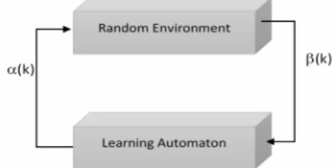
Learning Automata (LA) [44] is an adaptive decision making unit which is able to learn and improve its performance by choosing the optimal action from a limited set of actions. For a given action-set, there is also a probability vector in LA. An action is firstly selected according to the probability vector and then apply it to the random environment as an input. The environment evaluates the received action and responds with a reinforcement signal. The probability vector is updated according to the reaction from the environment. The main purpose in LA is to select the best action from the action-sets to minimize the average penalty received from the environment. LA is commonly used in complex, dynamic, and random systems where the accurate and complete information on the environment is not available [45]. Fig. 1 shows the relationship between random environment and learning automata.
Figure 1. Relationship between learning automata and its random environment
A random environment can be represented by a triple E={α,β,c}, α={α1,α2,…,αr} is a finite set of inputs (actions) and β={β1,β2,…,βm}represents the set of random outputs. In other words, β is the set of values that can be taken by the reinforcement signal, and c = {c1, c2 …, cr} is the set of penalty probabilities (these probabilities are calculated on the basis of the environment reaction), where the element ci is related to the action ai. The environment can be divided into stationary and non-stationary based on the type of penalty probabilities. In the stationary random environment, the penalty probabilities are fixed, while in a non-stationary environment these probabilities change with time. According to the nature of the reinforcement signal β, the random environment can be classified into three models P-model, Q-model and S-model. The P-model is referred to an environment in which the reinforcement signal can only take two binary values one and zero. The Q-model is an environment in which a limited number of values in [0, 1] are taken by the reinforcement signal. In an S-model environment, the reinforcement signal is a continuous random variable in the interval [a, b]. LA is divided into two main groups fixed structure LA and variable structure LA. In the fixed structure LA, transition and output functions are time-invariant, and the transition probability from one state to another and the actions and states selection probability are fixed. There are several examples of the FSLA, such as the Automaton of Tsetline, Krinsky, TsetlineG, and Krylov [46, 47]. The variable structure LA is denoted by {α , β, p, T}, where α={α1,α2,…,αr} is a finite set of actions, β={β1,β2,…,βm} is a set of inputs, p = {p1, p2, ..., pr} is the probability vector and p(k+1)=T[α(k),β(k),p(k)] is a learning algorithm. The learning algorithm is a recursive relationship correcting the action probability vector according to the responses. Let αi(k)∈α be an action selected by the learning automaton at the instant k, and p(k) be the probability vector of the action-set at the instant k. Thus, if αi receives a satisfactory response from the environment, pi(k) increases and probabilities of the others decrease, otherwise, pi(k) decreases and the probabilities of the rest increase. In each case, the changes are made so that the sum of pi(k) being kept equal to one. At each instant k, if the selected action αi(k) receives a reward from the random environment, the action probability vector p(k) is updated as follows:
+ 1 = 1 −+ 1 − ∀ ≠ 1 =
and if the selected action is penalized, the probability vector is updated by:
+ 1 = 1 − = − 1 + 1 − ∀ ≠ 2
where a and b are the reward and penalty parameters respectively, the increase or decrease in the probability of the actions is determined by the environment response, and r is the number of actions in the action-set. Therefore we may have three cases corresponding to the values of a and b. If (a = b), the above relations are called linear reward-penalty (LR-P) algorithm. If (a >> b), the equations are called linear reward-∈penalty (LR−∈P), and if b is zero (b = 0), they are called linear
reward-inaction (LR−I). If the selected action in the LR-I, is penalized by the environment, the action probability vector remains unchanged because of the zero value of b.
A. Variable Action Set Learning Automata
A variable action-set learning automaton (VLA) is an automaton in which the number of the available actions change with the time. A VLA contains a finite set of n actions as α={α1,α2,…,αn}. A={A1,A2,…,Am} indicates the set of action subsets and A(k)⊆α shows a subset of all the actions that can be selected by the learning automaton at the instant k. The particular action subsets are randomly selected by an external agency according to the probability distribution of Ψ(k) ={Ψ1(k),Ψ2(k),…,Ψm(k)} which is defined over possible subsets of the actions:
Ψ = [ = | ∈ , 1 ≤ ≤ 2!− 1] # = [$ = $ | , $ ∈ ] is the probability of choosing αi if the action subsets A(k) has already been selected and αi belongs to A(k) (αi∈A(k)). The value of the scaled probability ̂ is calculated by
̂ = & 3
where & = ∑)*∈+ , is the sum of actions
probabilities in A(k) and = [$ = $ ].
The method of choosing an action and updating the probability of actions in a variable-action-set learning automaton can be described as follows. First, we assume that A(k) is the subset of the selected action at the instant k. Before selecting an action from A(k), the probability of all actions in the selected subset are calculated by using Eq. (3). Then the automaton chooses one of the actions in A(k) randomly according to the scaled action probability vector ̂ . Depending on the received response from the environment, the learning automaton updates its scaled action probability vector. Of course, it should be noted that only the probabilities of the actions in the selected subset will be updated. Finally, the probability vector of the actions of the selected subset is re-scaled by
+ 1 = ̂ + 1 ∗ & for all $∈A k 4
See [48] for more details.
IV. PROPOSED ALGORITHM
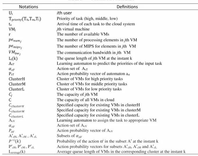
In this section, a learning automata-based algorithm, called LABTS, is proposed for the task scheduling problem on virtual machines in the cloud environment. In this approach, the scheduling is supposed to be online, i.e. the tasks are scheduled individually corresponding to the arrival time which is thus a non-preemptive scheduling method i.e. the processing of a task on a virtual machine is not stopped until its execution be completed. To understand the proposed algorithm better, we describe the parameters, the mathematical model, and problem definition in the sequel. TABLE I shows the most used notation and parameters.
TABLE I. NOTATIONS AND PARAMETERS
Notations
Definitions
Ui
i
th user
T
priorityT
h,T
m,T
l Priority of task (high, middle, low)ta Arrival time of each task to the cloud system
VMj jth virtual machine
r The number of available VMs
A!BCD The number of processing elements in jth VM
AC EFD The number of MIPS for elements in jth VM
GHIJD The communication bandwidth in jth VM
Ljk The queue length of jth VM at the instant k
AsT Learning automaton to predict the priorities of the input task
$FM Action-set of AsT
PsT Action probability vector of automaton ast
ClusterH Cluster of VMs for high priority tasks
ClusterM Cluster of VMs for middle priority tasks
ClusterL Cluster of VMs for low priority tasks
S The capacity of jth VM
C The capacity of all VMs in cloud
STUBFVWXY Specified capacity for existing VMs in clusterH
STUBFVWXZ Specified capacity for existing VMs in clusterM
STUBFVWX[ Specified capacity for existing VMs in clusterL
AsV Learning automaton to assign the task to appropriate VM
$F\ Action-set of AsV
]F\ Action probability vector of AsV
A′cH, A′cM , A′cL Subsets of $F\
]′ Probability of the action αi in the subset A′ at the instant k P′cH, P′cM , P′cL Action probability vectors for subsets A′cH, A′cM and A′cL
Laverage(k) Average queue length of VMs in the corresponding cluster at the instant k
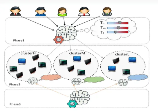
The proposed algorithm uses the learning automata to schedule tasks on virtual machines through Fixed set Learning Automaton and Variable Action-set Learning Automaton. The first learning automaton is used to predict the priority of input tasks and determines the probability of the tasks as high, middle and low. By knowing the probability of input tasks and given priorities, the virtual machines are clustered into three clusters, each of which are assigned to one of the tasks’ priorities. Using the Variable Action-set Learning Automaton, tasks are assigned to virtual machines in each cluster. The virtual machines are re-clustered according to the priority probability of tasks and after entering a certain number of tasks. In this model, the users (U1, U2, U3 … Un) send their tasks to the cloud system for execution and it is always expected VMs to be assigned as required. The priority of each task, Tpriority can be categorized into three classes high (Th), middle (Tm) and low (Tl) accordingly [29]. The arrival time of each task to the cloud system is shown by ta. VM= {VM1, VM2…, VMr} is a set of virtual
machines assigned to tasks that are sent to the cloud system over time. Each virtual machine has several features, namely, the number of processing elements, the number of millions instructions per second (MIPS) for these elements, and the communication bandwidth in each virtual machine which are denoted by penum, pemips and VMbw, respectively. Additionally, each virtual machine has a waiting queue that assigned tasks remained in queue until be executed by it. Thus, L(k) is
the length of the queue, the number of tasks, in each virtual machine at the instant k.Therefore the LABST algorithm can be divided into three main phases shown in Fig. 2.
A. Phase 1: predicting the priority of input tasks
In a cloud system, the user's requested tasks arrive at different times and are scheduled according to the scheduling algorithm which is online. Thus, once any task enters the system, the scheduling is executed by assigning it to an appropriate virtual machine. Tasks generally are with arrival times and different priorities. In this algorithm, three priorities as high, middle and low are considered for the tasks. The volume of input tasks with different priorities can vary over time. That is, in a special time interval, high-priority tasks are more requested by users, and the tasks with a middle or low priority will enter the system in the other intervals. Therefore, a predictive and learning method can be useful for predicting the priority of tasks. Thus a learning automaton named AsT is used in this phase that is able to predict the priorities of the input task. AsT is a Fixed Action-set Learning Automaton with three actions defined as $FM = {High, Middle, Low}. The selection of a priority from the action-set αsT is predicting the task priority entered into the cloud system according to the action probability vector of automaton AsT, shown as PsT={PsTh ,PsTm,PsTl}.
Figure 2. Schematic representation of the three phases
It is obvious that each priority is selected on the basis of their probability. All priorities in the action-set initially are with the same probability. Since AsT is a fixed action-set with three values, then the probability of selecting each action is equal tod c.
In this phase, when a new task enters the cloud (represented by Tnew), the automaton AsT selects one of the actions from the action-set randomly based on the action probability vector. If the task priority entered into the cloud is equal to the selected priority from the action-set, then it indicates that the selected action is correctly predicted and its probability increases by Eq. (1). However, if the priority of the input task is not the same the selected, then the probability of the action selected from the action-set of automaton AsT is reduced by Eq. (2). Therefore, this phase is executed upon the arrival of each task and the priority prediction improves over time. Because by giving reward to the correct predictions and considering penalty for inaccurate predictions, the action probability vector of the automaton AsT is updated and these values are changed corresponding to the environment responses. The pseudo code of phase 1 (predicting the priority of input tasks) is shown in TABLE II.
TABLE II. THE PSEUDO CODE OF PHASE 1 IN LABST ALGORITHM
Phase 1: predicting the priority of input tasks
,Tnew
sT
Input: P
sT
Output: P
rnd=random(0,1)
1
if (rnd<=]FMe) then 2
Select_Action← High 3
else if (]FMe< rnd<=]FMe+]FMC) then 4
Select_Action← Middle
5
else 6
Select_Action← Low 7
end if 8
if ( Select_Action ==Tnewpriority )
9
) 1 ( with Eq.
sT
Update P
10
else 11
(2) Eq. with
sT
Update P
12
end if 13
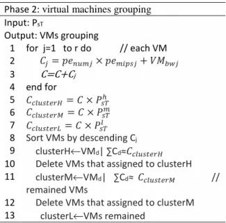
B. Phase 2: virtual machines grouping
After predicting the priority of input tasks, the grouping phase is started to group virtual machines corresponding to the action probability vector obtained from the previous step. In this phase, virtual machines are classified into three clusters, the first of which is for high priority tasks (clusterH), the second one for middle priority tasks (clusterM) and the third cluster for low priority tasks (clusterL). In the first phase, the action probability vector of AsT is changed based on the priority of the input tasks and the amount of rewards or penalties. Additionally, the arrival of only one task does not lead to significant changes in the action probability vector. Therefore the grouping phase is not repeated at the entry of each task and re-grouping is performed when a certain number of tasks enter. For example, after entering 10 tasks, the re-grouping is performed based on the new value of the action probability vector PsT, which can be determined by the cloud system. In this phase, virtual machines are grouped based on the action probability vector PsT. To perform grouping According to the characteristics of each virtual machine, the capacity of each machine [29] is first calculated by
S = A!BC f AC EF + GHIJ 5 Therefore, the capacity of all virtual machines in the cloud can be defined as:
S = h S X ic
6
After calculating the capacity of each virtual machine and the capacity of all virtual machines by Eq. (5) and Eq.(6) respectively, the capacity of each cluster is calculated according to the action probability vector PsT, which is defined as follows:
STUBFVWXY= S f ]FMe STUBFVWXZ= S f ]FMC
STUBFVWX[= S f ]FMU (7) ]FMe + ]FMC+ ]FMU = 1 , then S = STUBFVWXY+ STUBFVWXZ+ STUBFVWX[. After calculating the capacity of each cluster, virtual machines should be placed in the clusters accordingly. The clusterH is used for assigning high priority tasks with the highest priority. Thus the first virtual machines fall into cluster clusterH accordingly which is the same as STUBFVWXY .Thus the virtual machines are arranged in descending order according to their capacity. Virtual machines with the highest capacity are placed in the clusterH with a total capacitySTUBFVWXY . Then, these virtual machines are removed from the list of existing virtual machines, and those with the highest capacity and total capacity equal to STUBFVWXZ are selected among the remaining virtual machines to be placed in the clusterM. Finally, the remaining machines in the list are placed in clusterL. The aim in this phase, is to allocate machines with higher capability and lower queue length to the high priority tasks as well as reducing the waiting time for tasks with a middle and low priority. The pseudo code of phase 2 (virtual machines grouping) is shown in TABLE III.
TABLE III. THE PSEUDO CODE OF PHASE 2 IN LABST ALGORITHM
C. Phase 3: task scheduling on virtual machines in each cluster
After grouping virtual machines in the clusterH, clusterM, and clusterL, each task enters the cloud system and is sent to its corresponding cluster according to its priority. The learning automaton AsV is used to assign the task to the appropriate virtual machine in each cluster. This automaton has finite actions r, but the
number of actions may change at any time since the virtual machines in each cluster form the action-set of given automaton that is changed after grouping. Thus, the learning automation AsV is a Variable Action-set Learning Automaton.
First, all virtual machines in the VM list form the action-set of AsV, which is denoted by $F\= {$F\|∀GH ∈ GH}. In other words, each of the existing actions in the action-set of the automaton AsV represents one of the virtual machines in the VM list. The VM list has r virtual machines with the same initial selection probability. Thus, the action probability vector of AsV is defined as]F\= k]F\l∀GH ∈ GHm, where at the beginning of the cloud operation, the probability of each virtual machine is equal to cX . After grouping phase, virtual machines in each cluster form a subset from the action-set of AsV. Therefore, the subsets of the automaton AsV are A′cH, A′cM and A′cL, being the set of virtual machines for clusterH, clusterM, and clusterL, respectively, denoted by ′TY= {$TY|∀GH ∈ nopqrA s}, ′TZ = {$TZ|∀GH ∈ nopqrA H} and
′T[= {$T[,l∀GH,∈ nopqrA t}. Each of A′cH, A′cM and A′cL is a subset of $F\, with no elements in common because they are placed in different clusters in grouping phase, i.e. ′TY∩ ′TZ∩ ′T[= ∅. After determining the three subsets A′cH, A′cM and A′cL, the action probability vector in each subsetis calculated by Eq.(3) as follows:
]′ =∑ ] ]
)*w+′ , 8
Where P′i (k) is the probability of the action αi in the subset A′ at the instant k and Pi(k) is the action
probability ( ] = [$ = $ ] ) and
∑)*w+′ , ] is the sum of the probabilities of all actions in the subset A′.
P′cH, P′cM and P′cL are the updated action probability vectors calculated by Eq. (8) for subsets A′cH, A′cM and A′cL respectively which are defined as ]′TY= k]′TYl∀$ ∈ ′TYm, ]′TZ= k]′TZl∀$ ∈ ′TZm, and
]′T[= {]′T[, l∀$,∈ ′T[}. When a new task enters into each cluster according to its priority, all virtual machines in the corresponding cluster are a candidate to be assigned to the task. Thus, one of the actions in a given subset (which represents a virtual machine in the cluster) is selected based on the updated probability vector. If the queue length of the selected virtual machine is smaller or equal to the Laverage in the given cluster at current instant, the probability of the selected action and other actions in the subset is calculated by Eq. (1), which means receiving a reward related to the selected action and it assigned to the task, otherwise, the action probability vector is updated using Eq. (2), which means a penalty for the selected action and this phase continues. Laverage(k) shows the average queue length of VMs in the corresponding cluster at the instant k, which is computed as:
tyzWXy{W =∑ t
|+′ | ic
| ′ | , ∀$ | ′ 9
Phase 2: virtual machines grouping
Input: PsT
Output: VMs grouping
for j=1 to r do // each VM 1
S = A!BC f AC EF + GHIJ
2
C=C+Cj 3
end for 4
STUBFVWXY = S f ]FMe 5
STUBFVWXZ= S f ]FMC 6
STUBFVWX[ = S f ]FMU 7
Sort VMs by descending Cj 8
clusterH←VMd| ∑Cd≈STUBFVWXY 9
Delete VMs that assigned to clusterH
10
clusterM←VMd| ∑Cd≈ STUBFVWXZ //
remained VMs
11
Delete VMs that assigned to clusterM
12
clusterL←VMs remained
13
where A′ is one of the three subsets A′cH, A′cM and A′cL and A′ denotes the number of actions in the given subset. Li(k)is the queue length of each virtual machine in the action subset A′. After assigning the predefined number of input tasks to virtual machines, the grouping phase is required to be performed again because of changes in the action probabilities in the action probability vector of the automation AsT and changes in the arrival rate of tasks with different priorities. In this case, the action probability vectors must be calculated using Eq. (4) and the action vector of each action subset is updated once again after performing the grouping and determining the action subsets of each cluster. The pseudo code of phase 3 in LABST algorithm is shown in TABLE IV.
TABLE IV. THE PSEUDO CODE OF PHASE 3 IN LABST ALGORITHM
In the third phase of the proposed algorithm, the new task is sent to clusterH, clusterM and clusterL according to its priority High, Middle, and Low, respectively. In the first line of the pseudo-code, the value of the action vector of A′ is updated by Eq. (8) which takes place only after the grouping phase upon the determination of the action subsets. If there is no re-grouping, then there is no need to perform the first line because the subset of actions assigned to the cluster remains unchanged.
V. EXPERIMENT RESULTS
There are several issues such as network flow, virtual machine load balancing, scalability, management, etc. in a cloud system, so that theyhave been generally investigated in different extents. Additionally, the cloud systems provide software and hardware services on different scales by using resource providers. Therefore it's not possible to use the real cloud system to perform experiments by various criteria in the cloud system. Thus, it is essential to have a good simulator for testing and obtaining the results. One of these simulators is the cloudsim designed by the University of Melbourne, Australia in 2009 which is based on Java [49]. Cloudsim is a generalized simulator
allowing to model, simulate and test on cloud computing infrastructure and application services [50, 51]. There are four-layer architectures Simjava, gridsim, cloudsim and usercode first two of which are combined in a new architecture.
In this section, we analyze the efficiency of our proposed algorithm through simulation results performed by the cloudsim simulator in cloudsim-3.0.3 on a system with Intel corei5 processor, ram 6G and the windows 8.1 enterprise. Due to the importance of scalability, we consider the cloud system in three different sizes with different number of virtual machines. The small scale cloud system consists of 10 virtual machines, the medium scale cloud system consists of 25 virtual machines and a large-scale one has 50 VMs. In order to compare the LABTS algorithm with other algorithms, the number of tasks sent to each cloud systems by the user are 200, 600 and 1000.
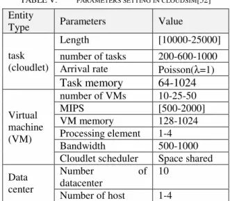
To validate the simulation, the instance types provided by Amazon Ec2, such as t2 and M5, are used. The simulation is performed on 10 data centers and the number of hosts for data centers varies from 1 to 4. These hosts are with different characteristics and the number of virtual machines per host is 3 and the number of PEs varies from 1 to 4. Virtual machines have a different processing power in the cloud environment, and MIPS (million instructions per second) ranges through [500-2000]. Priority of tasks are generated by a uniform distribution. The user’s task arrival distribution is Poisson with λ=1 indicating that the average number of tasks arrive to the cloud by user at each second is 1. To perform the test, tasks with different lengths are generated in the interval [10,000 - 25,000] by using a uniform distribution according to[52] . Tasks are independent of each other and the execution time of each task is not dependent on the previous or the next task. The simulation details are shown in TABLE V.
TABLE V. PARAMETERS SETTING IN CLOUDSIM[52]
To illustrate the effectiveness of the LABST scheduling algorithm, the values of makespan and the degree of imbalance obtained in simulation are compared with the results of some algorithms such as FCFS (First Come First Serve), Min-Min and HBB-LB [29].
Phase 3: task scheduling on virtual machines in each cluster
Input: Tnew , cluster Output: assign VM to Tnew
Update P′ with Eq.(8) //only after grouping phase
1
Select an action(VM) based on probability vector
2
if (VM(L(k))<=Laverage(k))
3
Assign selected VM to Tnew and update length of VM (L(k))
4
Update P′ with Eq. (1)
5
else 6
Update P′ with Eq. (2)
7
Go to 2
8
end if
9
Entity
Type Parameters Value
task (cloudlet)
Length [10000-25000]
number of tasks 200-600-1000
Arrival rate Poisson(λ=1)
Task memory
64-1024
Virtualmachine (VM)
number of VMs 10-25-50
MIPS [500-2000]
VM memory 128-1024
Processing element 1-4
Bandwidth 500-1000
Cloudlet scheduler Space shared Data
center
Number of
datacenter
10
Number of host 1-4
A. Makespan
Makespan is one of the important qualitative parameters in the cloud scheduling that shows the total length of the schedule (when all tasks have finished processing). In other words, makespan is the maximum value among the completion time of all tasks sent to the cloud. It is a basic parameter for evaluating scheduling algorithms that can be calculated according to Eq. (10).
H Aq ~ = H •∈VyF,F{€ ~ qℎ_r ƒA } 10 Where the finish_time denotes the end time of task i. Minimizing this parameter indicates that tasks are executed in the shortest possible time with no long waiting time.
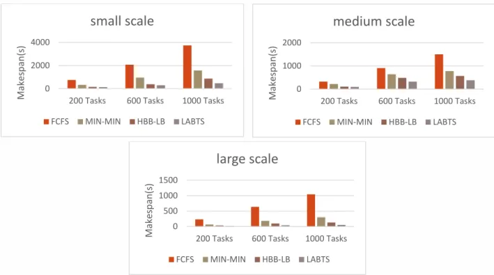
In order to calculate makespan, some scheduling algorithms, namely, FCFS, MIN-MIN, HBB-LB and LABTS are simulated through three scales: small scale with 10 VMs, medium scale with 25 VMs and large one with 50 VMs, with 200, 600 and 1000 tasks. In performing simulations, due to the use of random numbers for some parameters, each experiment is repeated 30 times and the final results are the average of 30 simulation runs. Fig. 3 illustrates the results of simulation for 200, 600, and 1000 tasks on small, medium, and large scale cloud systems. In the small scale, the number of virtual machines is low as compared to the user’s tasks with a Poisson arrival rate of λ=1. Thus its makespan is greater than other ones obtained at medium and large scales while the proposed algorithm has less makespan compared to the other scheduling methods. Because the algorithm uses the learning method to predict the type of tasks entering the cloud and assigning virtual machines to the tasks. By increasing the number of input tasks, the AsT learning algorithm will update the action probability vector, and thus more accurate predictions are made over time,
which also effects on the virtual machines grouping. Also, by updating the action probability vector of AsV, virtual machines with lower queue lengths are with larger probabilities more likely to be assigned to the tasks.
By comparing the methods FCFS, MIN-MIN, HBB-LB and the proposed algorithm LABTS in three scales small, medium, and large with 200, 600 and 1000 tasks shows that the makespan of the proposed method is significantly lower than other methods. In the LABTS method, it is expected that the makespan be lower than other methods because in LABTS, virtual machines are classified into clusters according to their capacity and capability, and tasks are sent to these clusters according to their priority type. On the other hand, grouping is performed in terms of predictions obtained by the learning automata. In the proposed approach, the migration of tasks is not required since by re-grouping and updating the probability vector of Learning Automaton AsV, tasks are assigned to the right virtual machines according to their priorities.
B. Degree of imbalance (DI)
Another important parameter in load balancing of virtual machines is the degree of imbalance (DI)[53], which is calculated in simulations to compare the LABTS with FCFS, MIN-MIN, and HBB-LB methods. DI, which shows the distribution of load balancing on virtual machines, is calculated by [29]
…† =‡Cyˆ‡− ‡C !
yz{ 11
where Tmax and Tmin are the maximum and minimum values of Ti among all virtual machines respectively and Tavg is the mean value of Ti in VMs.
Figure 3. Evaluating the makespan parameter resulting from the execution of 200, 600, and 1000 tasks in a cloud environment w ith small, medium and large scales
0 2000 4000
200 Tasks 600 Tasks 1000 Tasks
M
a
k
e
sp
a
n
(s
)
small scale
FCFS MIN-MIN HBB-LB LABTS
0 1000 2000
200 Tasks 600 Tasks 1000 Tasks
M
a
k
e
sp
a
n
(s
)
medium scale
FCFS MIN-MIN HBB-LB LABTS
0 500 1000 1500
200 Tasks 600 Tasks 1000 Tasks
M
a
k
e
sp
a
n
(s
)
large scale
FCFS MIN-MIN HBB-LB LABTS
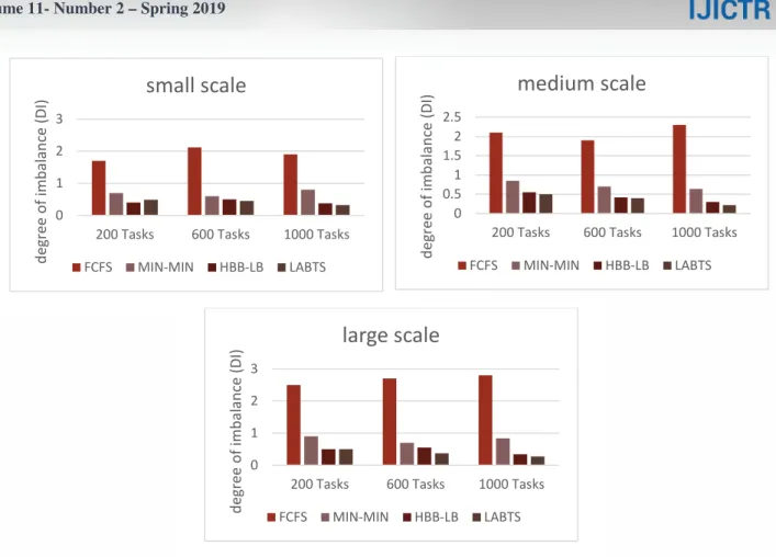
Figure 4. Evaluating the DI parameter resulting from the execution of 200, 600, and 1000 tasks in a cloud environment with small, medium and large scales
The value of Ti for each virtual machine is obtained by dividing the total length of assigned load to the machine by the machine's processing capacity, which indicates the required time of the virtual machine to perform its tasks. The value of DI parameter obtained from simulations in three cloud scales with 200, 600 and 1000 tasks is shown in Fig. 4. Using the learning automata, the proposed LABTS algorithm compared to FCFS, MIN-MIN, and HBB-LB methods provides more load balancing and is more efficient. Because there is no task migration between virtual machines in LABTS and the selection of appropriate virtual machines to be assigned to tasks is performed just by updating the action probability vector. Therefore, the more the number of tasks, the greater the learning. This increases the probability of accurate selection that helps to have a balanced distribution of tasks on virtual machines.
VI. CONCLUSION
In this paper, a learning automata-based task scheduling algorithm (LABTS) is presented for cloud environment. This algorithm not only performs the task scheduling on virtual machines, but also takes into account the priority of tasks in scheduling. Using predictive methods generally requires large memory location to store previous states along with taking more time to search between saved states, while a learning automaton predicts future states without storing previous states and just needs the probability vector be updated.In this paper, two learning automata are used for task scheduling on virtual machines. In the first phase, the first learning automaton is used to predict the priority of the tasks sent to the cloud, which has a fixed
action-set and the action probability vector is updated by receiving each task. In the second phase, the proposed algorithm divides virtual machines into three clusters in terms of the action probability vector. In the third phase, another learning automaton is used to assign each task to the appropriate virtual machine with variable action-set. To illustrate the efficiency of the LABTS algorithm, the simulations are performed in three scales small, medium, and large in cloudsim simulator. According to the numerical results obtained from the simulations, the proposed LABTS algorithm compared to FCFS, MIN-MIN, and HBB-LB algorithms performs significantly better in terms of makespan and DI.
REFERENCES
[1] R. Buyya, C.S. Yeo, S. Venugopal, J. Broberg, and I. Brandic, “Cloud computing and emerging IT platforms: Vision, hype, and reality for delivering computing as the 5th utility”, Future Generation Computer Systems, vol. 25, no. 6, pp. 599-616, 2009.
[2] P. Mell, and T. Grance, “The NIST definition of cloud computing”, Communications of the ACM, vol. 53, no. 6, pp. 50, 2010.
[3] S. Singh, and I. Chana, “QRSF: QoS-aware resource scheduling framework in cloud computing”, The Journal of Supercomputing, vol. 71, no. 1, pp. 241-292, 2015.
[4] L.F. Bittencourt, E.R. Madeira, and N.L. Da Fonseca, “Scheduling in hybrid clouds”, IEEE Communications Magazine, vol. 50, no. 9, 2012.
[5] J. Wu, X. Xu, P. Zhang, and C. Liu, “A novel multi-agent reinforcement learning approach for job scheduling in Grid computing”, Future Generation Computer Systems, vol. 27, no. 5, pp. 430-439, 2011.
[6] B.P. Rimal, A. Jukan, D. Katsaros, and Y. Goeleven, “Architectural requirements for cloud computing systems: an 0
1 2 3
200 Tasks 600 Tasks 1000 Tasks
d
e
g
re
e
o
f
im
b
a
la
n
ce
(
D
I)
small scale
FCFS MIN-MIN HBB-LB LABTS
0 0.5 1 1.5 2 2.5
200 Tasks 600 Tasks 1000 Tasks
d
e
g
re
e
o
f
im
b
a
la
n
ce
(
D
I)
medium scale
FCFS MIN-MIN HBB-LB LABTS
0 1 2 3
200 Tasks 600 Tasks 1000 Tasks
d
e
g
re
e
o
f
im
b
a
la
n
ce
(
D
I)
large scale
FCFS MIN-MIN HBB-LB LABTS
enterprise cloud approach”, Journal of Grid Computing, vol. 9, no. 1, pp. 3-26, 2011.
[7] F. Wu, Q. Wu, and Y. Tan, “Workflow scheduling in cloud: a survey”, The Journal of Supercomputing, vol. 71, no. 9, pp. 3373-3418, 2015.
[8] J. Yu, and R. Buyya, “A taxonomy of scientific workflow systems for grid computing”, ACM Sigmod Record, vol. 34, no. 3, pp. 44-49, 2005.
[9] O. Sonmez, N. Yigitbasi, S. Abrishami, A. Iosup, and D. Epema, “Performance analysis of dynamic workflow scheduling in multicluster grids”, Proceedings of the 19th ACM International Symposium on High Performance Distributed Computing, ACM, 2010, pp. 49-60.
[10] S. Smanchat, and K. Viriyapant, “Taxonomies of workflow scheduling problem and techniques in the cloud”, Future Generation Computer Systems, vol. 52, pp. 1-12, 2015. [11] L.F. Bittencourt, and E.R.M. Madeira, “HCOC: a cost
optimization algorithm for workflow scheduling in hybrid clouds”, Journal of Internet Services and Applications, vol. 2, no. 3, pp. 207-227, 2011.
[12] H.M. Fard, R. Prodan, J.J.D. Barrionuevo, and T. Fahringer, “A Multi-objective Approach for Workflow Scheduling in Heterogeneous Environments”, 12th IEEE/ACM International Symposium on Cluster, Cloud and Grid Computing (ccgrid 2012), 2012, pp. 300-309.
[13] M. Mezmaz, N. Melab, Y. Kessaci, Y.C. Lee, E.G. Talbi, A.Y. Zomaya, and D. Tuyttens, “A parallel bi-objective hybrid metaheuristic for energy-aware scheduling for cloud computing systems”, Journal of Parallel and Distributed Computing, vol. 71, no. 11, pp. 1497-1508, 2011.
[14] F. Tao, Y. Feng, L. Zhang, and T.W. Liao, “CLPS-GA: A case library and Pareto solution-based hybrid genetic algorithm for energy-aware cloud service scheduling”, Applied Soft Computing, vol. 19, pp. 264-279, 2014.
[15] X. Zuo, G. Zhang, and W. Tan, “Self-adaptive learning PSO-based deadline constrained task scheduling for hybrid IaaS cloud”, IEEE Transactions on Automation Science and Engineering, vol. 11, no. 2, pp. 564-573, 2014.
[16] Z. Wu, Z. Ni, L. Gu, and X. Liu, “A revised discrete particle swarm optimization for cloud workflow scheduling”, Computational Intelligence and Security (CIS), 2010 International Conference on, IEEE, 2010, pp. 184-188. [17] M.A. Tawfeek, A. El-Sisi, A.E. Keshk, and F.A. Torkey,
“Cloud task scheduling based on ant colony optimization”, 2013 8th International Conference on Computer Engineering & Systems (ICCES), 2013, pp. 64-69.
[18] P. Yi, H. Ding, and B. Ramamurthy, “A tabu search based heuristic for optimized joint resource allocation and task scheduling in grid/clouds”, Advanced Networks and Telecommuncations Systems (ANTS), IEEE International Conference on, IEEE, 2013, pp. 1-3.
[19] G.-n. Gan, T.-l. Huang, and S. Gao, “Genetic simulated annealing algorithm for task scheduling based on cloud computing environment”, Intelligent Computing and Integrated Systems (ICISS), International Conference on, IEEE, 2010, pp. 60-63.
[20] F. Palmieri, L. Buonanno, S. Venticinque, R. Aversa, and B. Di Martino, “A distributed scheduling framework based on selfish autonomous agents for federated cloud environments”, Future Generation Computer Systems, vol. 29, no. 6, pp. 1461-1472, 2013.
[21] J. Yu, R. Buyya, and K. Ramamohanarao, Workflow Scheduling Algorithms for Grid Computing, Springer Berlin Heidelberg, Berlin, Heidelberg, 2008.
[22] J. Yu, and R. Buyya, “Scheduling scientific workflow applications with deadline and budget constraints using genetic algorithms”, Scientific Programming, vol. 14, no. 3-4, pp. 217-230, Dec. 2006.
[23] F. Ramezani, J. Lu, and F. Hussain, “Task scheduling optimization in cloud computing applying multi-objective particle swarm optimization”, International Conference on Service-oriented computing, Springer, 2013, pp. 237-251. [24] N. Netjinda, B. Sirinaovakul, and T. Achalakul, “Cost optimal
scheduling in IaaS for dependent workload with particle swarm
optimization”, The Journal of Supercomputing, vol. 68, no. 3, pp. 1579-1603, 2014.
[25] S. Parthasarathy, and C.J. Venkateswaran, “Scheduling jobs using oppositional-GSO algorithm in cloud computing environment”, Wireless Networks, vol. 23, no. 8, pp. 2335-2345, 2017.
[26] L. Liu, H. Mei, and B. Xie, “Towards a multi-QoS human-centric cloud computing load balance resource allocation method”, The Journal of Supercomputing, vol. 72, no. 7, pp. 2488-2501, 2016.
[27] A. Salehan, H. Deldari, and S. Abrishami, “An online valuation-based sealed winner-bid auction game for resource allocation and pricing in clouds”, The Journal of Supercomputing, vol. 73, no. 11, pp. 4868-4905, 2017. [28] A. Nezarat, and G. Dastghaibyfard, “A game theoretical model
for profit maximization resource allocation in cloud environment with budget and deadline constraints”, The Journal of Supercomputing, vol. 72, no. 12, pp. 4737-4770, 2016.
[29] D.B. L.D, and P. Venkata Krishna, “Honey bee behavior inspired load balancing of tasks in cloud computing environments”, Applied Soft Computing, vol. 13, no. 5, pp. 2292-2303, 2013.
[30] D. Ergu, G. Kou, Y. Peng, Y. Shi, and Y. Shi, “The analytic hierarchy process: task scheduling and resource allocation in cloud computing environment”, The Journal of Supercomputing, vol. 64, no. 3, pp. 835-848, 2013.
[31] S.K. Mishra, D. Puthal, B. Sahoo, S.K. Jena, and M.S. Obaidat, “An adaptive task allocation technique for green cloud computing”, The Journal of Supercomputing, DOI, pp. 1-16, 2018.
[32] Z. Wang, and X. Su, “Dynamically hierarchical resource-allocation algorithm in cloud computing environment”, The Journal of Supercomputing, vol. 71, no. 7, pp. 2748-2766, 2015.
[33] A. Deldari, M. Naghibzadeh, and S. Abrishami, “CCA: a deadline-constrained workflow scheduling algorithm for multicore resources on the cloud”, The journal of Supercomputing, vol. 73, no. 2, pp. 756-781, 2017.
[34] A. Hanani, A.M. Rahmani, and A. Sahafi, “A multi-parameter scheduling method of dynamic workloads for big data calculation in cloud computing”, The Journal of Supercomputing, vol. 73, no. 11, pp. 4796-4822, 2017. [35] S. Singh, and I. Chana, “Resource provisioning and scheduling
in clouds: QoS perspective”, The Journal of Supercomputing, vol. 72, no. 3, pp. 926-960, 2016.
[36] D. Ding, X. Fan, and S. Luo, “User-oriented cloud resource scheduling with feedback integration”, The Journal of Supercomputing, vol. 72, no. 8, pp. 3114-3135, 2016. [37] J.A. Torkestani, “A new approach to the job scheduling
problem in computational grids”, Cluster Computing, vol. 15, no. 3, pp. 201-210, 2012.
[38] S. Sahoo, B. Sahoo, and A.K. Turuk, “An Energy-Efficient Scheduling Framework for Cloud Using Learning Automata”, 2018 9th International Conference on Computing, Communication and Networking Technologies (ICCCNT), IEEE, 2018, pp. 1-5.
[39] S. Sahoo, B. Sahoo, and A.K. Turuk, “A Learning Automata-based Scheduling for Deadline Sensitive Task in The Cloud”, IEEE Transactions on Services Computing, DOI, 2019. [40] S. Misra, P.V. Krishna, K. Kalaiselvan, V. Saritha, and M.S.
Obaidat, “Learning automata-based QoS framework for cloud IaaS”, IEEE Transactions on Network and Service Management, vol. 11, no. 1, pp. 15-24, 2014.
[41] M. Ranjbari, and J.A. Torkestani, “A learning automata-based algorithm for energy and SLA efficient consolidation of virtual machines in cloud data centers”, Journal of Parallel and Distributed Computing, vol. 113, pp. 55-62, 2018.
[42] A.A. Rahmanian, M. Ghobaei-Arani, and S. Tofighy, “A learning automata-based ensemble resource usage prediction algorithm for cloud computing environment”, Future Generation Computer Systems, vol. 79, pp. 54-71, 2018. [43] R.D. Venkataramana, and N. Ranganathan, “A learning
automata based framework for task assignment in heterogeneous computing systems”, Proceedings of the 1999
ACM symposium on Applied computing, Citeseer, pp. 541-547.
[44] K.S. Narendra, and M.A. Thathachar, Learning automata: an introduction, Courier Corporation2012.
[45] W. Jiang, C.-L. Zhao, S.-H. Li, and L. Chen, “A new learning automata based approach for online tracking of event patterns”, Neurocomputing, vol. 137, pp. 205-211, 2014.
[46] M.R. Meybodi, and H. Beigy, “New learning automata based algorithms for adaptation of backpropagation algorithm parameters”, International Journal of Neural Systems, vol. 12, no. 01, pp. 45-67, 2002.
[47] B. Johnoommen, “Absorbing and ergodic discretized two-action learning automata”, IEEE transtwo-actions on systems, man, and cybernetics, vol. 16, no. 2, pp. 282-293, 1986.
[48] M. Thathachar, and B.R. Harita, “Learning automata with changing number of actions”, IEEE transactions on systems, man, and cybernetics, vol. 17, no. 6, pp. 1095-1100, 1987. [49] T. Goyal, A. Singh, and A. Agrawal, “Cloudsim: simulator for
cloud computing infrastructure and modeling”, Procedia Engineering, vol. 38, pp. 3566-3572, 2012.
[50] R.N. Calheiros, R. Ranjan, A. Beloglazov, C.A. De Rose, and R. Buyya, “CloudSim: a toolkit for modeling and simulation of cloud computing environments and evaluation of resource provisioning algorithms”, Software: Practice and experience, vol. 41, no. 1, pp. 23-50, 2011.
[51] R.N. Calheiros, R. Ranjan, C.A. De Rose, and R. Buyya, “Cloudsim: A novel framework for modeling and simulation of cloud computing infrastructures and services”, arXiv preprint arXiv:0903.2525, DOI, 2009.
[52] N. Zekrizadeh, A. Khademzadeh, and M. Hosseinzadeh, “An Online Cost-Based Job Scheduling Method by Cellular Automata in Cloud Computing Environment”, Wireless Personal Communications, DOI, pp. 1-27, 2019.
[53] K. Li, G. Xu, G. Zhao, Y. Dong, and D. Wang, “Cloud task scheduling based on load balancing ant colony optimization”, Chinagrid Conference (ChinaGrid), Sixth Annual, IEEE, 2011, pp. 3-9.
Neda Zekrizadeh Received B.
Sc. degree in Software
Engineering from Islamic Azad University, Tabriz, IRAN in 2007. She also received her M.Sc. degree from Islamic Azad University, Tabriz, IRAN in 2010 in Computer Architecture Engineering. She is currently working toward the Ph.D. degree in Architecture Computer Engineering at the Science and Research Branch of Islamic Azad University, Tehran, IRAN (SRBIAU). Her current research interests include Distributed Systems, Scheduling and Resource Management in Cloud and Grid Networks.
Ahmad Khademzadeh was
born in Mashhad, Iran, in 1943. He received the B.Sc. degree in Applied Physics from Ferdowsi University, Mashhad, Iran, in 1969 and the M.Sc. and Ph.D. degrees respectively in Digital Communication and Information Theory and Error Control Coding from the University of Kent, Canterbury, UK. He is
currently a Full professor in ICT Research Institute (ITRC). He is a member of the Iranian Electrical Engineering Conference Permanent Committee. Dr. Khadem Zadeh has received four distinguished national and international awards including Kharazmi International Award, and has been selected as the national outstanding researcher of the Iran Ministry of Information and Communication Technology. His research interests include VLSI Design, Interconnection Network, Fault Tolerant and Computer Architectures.
Mehdi Hosseinzadeh received
his B.Sc. degree in Computer Hardware Engineering from Islamic Azad University, Dezful Branch, Iran in 2003. He also received the M.Sc. and Ph.D. degrees in Computer System Architecture from the Science and Research Branch, Islamic Azad University, Tehran, Iran in 2005 and 2008, respectively. He is currently an Associate Professor at Iran University of Medical Sciences, Tehran, Iran. His research interests are Information Technology, Data Mining, Big data Analytics, Commerce, E-Marketing and Social Networks.