45
A multi-objective resource-constrained project scheduling problem
with time lags and fuzzy activity durations
Alireza Eydi
1*, Mohsen Bakhshi
11Department of Industrial Engineering, University of Kurdistan, Sanandaj, Iran [email protected], [email protected]
Abstract
The resource-constrained project scheduling problem is to find a schedule that minimizes the project duration subject to precedence relations and resource constraints. To further account for economic aspects of the project, one may add an objective of cash nature to the problem. In addition, dynamic nature and variations in real world are known to introduce uncertainties into data. Therefore, this study is aimed at proposing a multi-objective model for resource-constrained project scheduling problem, with the model objectives being to minimize makespan, and maximize net present value of the project cash flows; the proposed model has activity times expressed in fuzzy numbers where the corresponding uncertainties are taken into account. The project environment is considered to be a multi-resource environment where more than one resource is needed for the execution of any activity. Also, the proposed model comes with time lags in precedence relations between activities. The proposed model is validated by using epsilon-constraint method. The α-cut approach as well as the expression of acceptable risk level by the project manager is used to defuzzificate fuzzy activity durations. Since the problem is NP-hard, a NSGA-II meta-heuristic algorithm is proposed to solve the problem. The algorithm performance has been evaluated in terms of different criteria.
Keywords: Resource-constrained project scheduling, fuzzy activity times, time lags,
cash flows, α-cut, NSGA-II evolutionary algorithm.1- Introduction
In project scheduling problems, on time and successful completion of the project is the most important objective to be considered in planning phase. Due to resource constraints and precedence relations, activities should be prioritized and planned in such a way to avoid any delay in the project completion. However, due to ambiguities and uncertainties in activity times, it is very difficult (and often impractical) to have them estimated precisely as such an estimation must well respond to different approaches and techniques in face of uncertainties; i.e., the estimation is to resolve uncertainties in such a way to not only prevent any delay in the project due date and excessive costs, but also to accelerate the project completion by setting optimal conditions.
Expressing time-related uncertainties and ambiguities in fuzzy numbers can somewhat resolve uncertain nature of the project time. Representing activity times in fuzzy numbers prevents the occurrence of unwanted delay risk which otherwise can lead the project to deviate from the developed implementation plan. Employing these numbers (and using α-cut to have the defuzzified subsequently) creates wider domain of starting times for different activities. The literature about scheduling under uncertainty indicates that use of fuzzy numbers is more preferred, compared to random variables (Herroelen and Leus, 2005).
*Corresponding author
ISSN: 1735-8272, Copyright c 2019 JISE. All rights reserved Journal of Industrial and Systems Engineering
Vol. 12, Special issue on Project Management and Control, pp. 45-71 Winter (January) 2019
46
The most important precedence relation in network diagram of activities is Finish-to-Start relationship. In many studies such as Kolisch and Hartmann (2006), it is considered to be zero, implying that any activity must be started immediately following the completion of its precedent activity. However, considering time lags in precedence relations between successive activities in the project network, one can come to a more realistic study of scheduling problems. With these lags considered in scheduling problems, an activity is not necessarily to start immediately following the completion of its precedent activity. Moreover, the lags can be used to prevent from violation from level of available resources. In total, it seems inevitable to apply these time lags between activities as, for instance, many equipment sets need some preparation and setup times to get ready for the execution of the next activity after the completion of the precedent one.
Primarily, in resource-constrained project scheduling problems (RCPSPs), the objective is to minimize the project makespan. However, this does not mean to ignore objectives related to cost and cash. Indeed, in order to strengthen economic aspects of the project, one may further takes into account objectives aiming at minimizing total costs while maximizing net present value (NPV) of project. This is the case with different types of resources including renewable and nonrenewable ones.
In this study, a new model is proposed to solve RCPSPs. The model is not only to minimize project duration, but also seeks to maximize the project NPV, representing a multi-objective problem. Herein, activity times are taken as fuzzy numbers with time lags considered between activities. The time lags are assumed to be closed intervals with their lower and upper bonds being the minimal and maximal time lags, respectively. Also, the project is considered to launch within a multi-resource environment.
Different solution approaches for multi-objective problems are classified into two classes: classic and evolutionary techniques. Classic or numerical methods go for converting a multi-objective problem into a set of single-objective ones via mathematical transformations. Evolutionary methods present a Pareto set of solutions and rely on an initial assumption that none of solutions in this set is absolutely better than the others. In fact, one solution is defined to dominate another one if, compared to the other solution, it is not worse in none of the objectives while being better in at least one of the objectives. In this study NSGA-II meta-heuristic is used and evolutionary algorithm which presents non-dominated solutions for achieving acceptable solutions within a reasonable time, with the results evaluated by a number of criteria and indicators.
Following with the paper, section 2 deals with a review on relevant literatures. Section 3 describes the mathematical model of the problem which is validated in Section 4. In section 5, the new approach is proposed and evaluated, with the computational results discussed in section 6. Finally, a summary of the paper together with a number of conclusions are provided in section 7.
2- Literature review
Project scheduling problems considering limited resources were first raised by Wiest (1962). Looking for the minimization of project completion time (as problem objective), Agarwal et al. (2007) presented a new approach to scheduling problems by planning and determining orders and priorities of activities based on resources constraints. In the following, the relevant researches are classified from four main characteristics.
2-1- Economic objective functions
Taking a multi-resource case including renewable and nonrenewable resources, for the first time, Nudtasomboon and Randhawa (1997) defined their problem objectives as minimizing the project completion time and cost as well as resource leveling. De Reyck and Herroelen (1998) studied RCPSPs with their aim being to maximize the project NPV, as the problem objective. Kazemi and Tavakkoli-Moghaddam (2011a) solved a model of RCPSP to minimize the project duration and maximize its NPV. Kalili et al. (2013) proposed a bi-objective scheduling problem wherein the project duration minimization along with NPV maximization was set as objectives. Leyman and Vanhoucke (2016) extended a new scheduling method and implemented within a genetic algorithm, which moves activities to improve the
47
project NPV. Moradi et al. (2018) studied a RCPSP based on the resource leveling problem. Results of the proposed model show that the subcontractors belong to a large-scale project can earn more profit by the cooperation.
2-2- Multi-objective scheduling model
Considering two objectives, namely minimizing total project time and maximizing surplus utilization of renewable sources, Davis et al. (1992) investigated approaches based on creating Pareto sets of solutions. In order to create Pareto fronts, Hapke, Jaszkiewicz, and Słowiński (1998) proposed a multi-criteria approach towards considering multiple objectives based on time, resources, and costs. Kazemi and Tavakkoli-Moghaddam (2011b) presented a multi-objective multi-mode RCPSP model based on minimal makespan and maximal NPV and had the model solved by NSGA-II algorithm. Vanucci et al. (2012) introduced a modified NSGA-II algorithm for obtaining solutions for a multi-objective RCPSP. Abello and Michalewicz (2014) investigated a dynamic version of the RCPSP where the number of tasks varies in time. Minimization of schedule cost and duration were the two objectives in their research. Ghamginzadeh et al. (2014) presented a multi-objective cuckoo algorithm to solve a multi-objective RCPSP with two objective functions: minimizing the project makespan and minimizing the project NPV. Berthaut et al. (2014) presented a model for the RCPSP with feasible overlapping modes. The makespan minimization and the gain maximization were objective functions in this research. Gomes et al. (2014) Studied the RCPS problem with precedence relations, and with two objective functions: minimizing the makespan and the total weighted start time of the activities. They proposed and analyzed five multi-objective metaheuristic algorithms to solve the problem. Xiao et al. (2016) extended an electromagnetism algorithm to solve a multi-objective RCPSP with two objective functions: optimizing the project makespan and the total tardiness.Maghsoudlou et al.(2016) studied a new multi-skill multi-mode RCPSP with three objectives: minimizing projects' makespan, minimizing total cost of allocating workers to skills, and maximizing total quality of processing activities. They developed multi-objective invasive weeds optimization algorithm (MOIWO) to solve the proposed problem. Elloumi et al. (2017) studied the multi-mode RCPSP with two objective functions: minimizing the project makespan and a disruption measures. Tritschler et al. (2017) proposed a metaheuristic based on a genetic algorithm for the RCPS problem with flexible resource profiles, and with minimizing the makespan. Tao and Dong (2018) considered multi-mode RCPS problem with alternative project structures. They developed a hybrid metaheuristic to solve a bi-objective linear programming, which minimizes the makespan and total cost. Wang and Zheng (2018) considered multi-skill RCPS problem. They developed a knowledge-guided multi-objective fruit fly optimization algorithm to solve a mixed-integer, bi-objective programming, which minimizes the makespan and total cost simultaneously.
In terms of solution approaches, different ranges of algorithms have been applied by various researchers. Moghal et al. (2016) developed a mixed-integer linear programming model for minimizing transportation costs and inventory of food grains in India, and also used a Chemical Reaction Optimization (CRO) algorithm for testing the model. Mogale et al. (2018) formulated a MINLP model for planning the food grain storage and movement from surplus states to deficit states considering the seasonal procurement, silo capacity, demand satisfaction, and vehicle capacity constraints. The formulated problem was solved by a Hybrid Particle-Chemical Reaction Optimization (HP-CRO) algorithm. Mogale et al. (2018) used Frank-Wolfe linearization technique along with Benders' decomposition method to solve the developed model. The decision making challenges in their model was whether to manufacture the common component centrally or locally. In another research, Mogale et al (2018) developed an integrated multi-objective, multi-modal and multi-period model for the grain silo location-allocation problem with dwell time. The formulated problem was solved by a Non-dominated Chemical Reaction Optimization (NCRO) algorithm.
2-3- Fuzzy scheduling model
Due to limited and insufficient availability of statistical data, it is difficult to apply probability theory to find an appropriate probability distribution for uncertainties in activity times. As of introducing the theory
48
of fuzzy sets by Zadeh in 1965, this issues was somewhat solved. Extending the studies by Zadeh, Dubois (1980) and Nahmias (1978) utilized fuzzy numbers theory as a useful tool to address associated uncertainties with data. Chanas and Zielinski (2001) undertook scheduling and determined critical path in project network by taking activity times as being fuzzy. Hapke, Jaszkiewicz, & Slowinski (1994) and Hapke and Slowinski (1996) were the first to present RCPSPs in fuzzy circumstances. Zhao et al. (2008) studied RCPSP using fuzzy numbers to represent activity times, introducing critical chain content for the first time. Atli and Kahraman (2014), not only considered different approaches to the execution of activities, proposed two separate models for activity times when taken as of determined and fuzzy natures, respectively. Hao et al. (2014) presented a stochastic multiple mode RCPSP with two objectives of minimizing the project completion time and maximizing the scheduling robustness. Palacio and Larrea (2016) presented a lexicographic approach based on two mixed-integer programming models to solve RCPSP. The first model aims to minimize makespan, while the second model maximizes the robustness the schedule. Habibi et al. (2017) proposed a multi-objective project scheduling model with time-varying resource requirements and capacities. They proposed two algorithms, NSGA-II and MOPSO, to solve the problem with the objective functions: minimizing the project makespan, maximizing the schedule robustness, and maximizing the NPV. Wieseman and Daniel (2015) reviewed the two major strands of literature on stochastic NPV maximization. Artigues et al. (2015) examined the RCPSP for the case when there is uncertainty in the activity durations.
2-4- precedence relationships with lags
Investigating different types of precedence relations between activities of the same project, Chassiakos and Sakellaropoulos (2005) considered time-cost tradeoffs in RCPSPs, so as to minimize time lags between activities. Demeulemeester and Herroelen (1996) further studied the application of minimum time lags for setup times of equipment. In addition to surveying RCPSPs with different modes for executing activities, Drexl et al. (2000) studied the dependency between minimum time lags and the different modes of activity implementation. Bartusch et al. (1988) investigated minimum time lags, considering maximum time lags between activities.
Ballestín (2007) developed a genetic metaheuristic algorithm for RCPSP with resource renting, in which minimum and maximum time lags were involved. Čapek et al. (2012) considered an extension of RCPS problem, in which one resource along with positive and negative time lags and sequence-dependent setup times was involved.
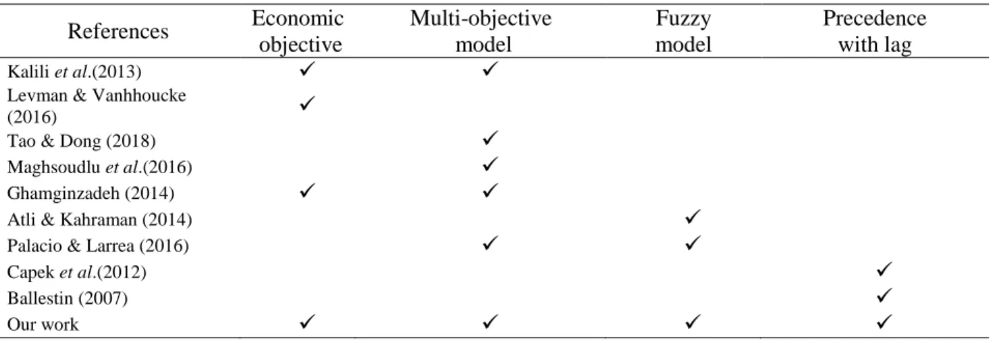
The literature and some characteristics related to the research problem on RCPSP were reviewed in the previous subsections. Some researches in this field are summarized in table 1 to present research gaps for this study.
Table 1. Findings of the literature RCPSP
References Economic
objective
Multi-objective model
Fuzzy model
Precedence with lag
Kalili et al.(2013)
Levman & Vanhhoucke
(2016)
Tao & Dong (2018)
Maghsoudlu et al.(2016)
Ghamginzadeh (2014)
Atli & Kahraman (2014)
Palacio & Larrea (2016)
Capek et al.(2012)
Ballestin (2007)
49
3- Problem definition and formulation
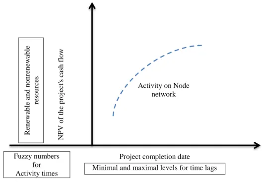
Here, the structure of the project is defined as an oriented graph of no loop, as represented by Activity on Node (AoN) network. The nodes represent project activities and the arcs serve as precedence relations between activities. Initial and final activities are dummy activities representing start and completion of the project, respectively. No activity starts immediately following the completion of its precedent, necessarily, and there exists minimal and maximal levels for time lags. The availability of a given resource will be fixed at a certain level for each period of the project horizon. The problem involves both renewable and nonrenewable resources. Activity times are expressed in triangular and trapezoidal fuzzy numbers. Project cash flows depend on start times of activities, with total cash inflows and outflows occurring at the start times. The idea of problem definition is depicted figure 1.
Fig. 1. The idea of problem definition
3-1- Parameters and decision variables
Sets and indicesi Index of activities 𝑖 = 1, 2, … , 𝑁
j Index of activities 𝑗 = 1, 2, … , 𝑁
P(i) Set of precedent activities of the ith activity
k Index of renewable resources 𝑘 = 1, 2, … , 𝐾
h Index of nonrenewable resources ℎ = 1, 2, … , 𝐻
Parameters
N number of activities CFi cash flow of the ith activity di duration time of the ith activity
ℓij minimum finish-to start time lag between activities i and j
NPV
o
f
th
e
p
ro
ject's c
ash
f
lo
w
R
en
ewa
b
le
an
d
n
o
n
ren
ewa
b
le
reso
u
rce
s
Activity on Node network
Project completion date
Minimal and maximal levels for time lags Fuzzy numbers
for Activity times
50 uij maximum finish-to start time lag between
activities i and j
rik the renewable resource requirement of activity i for resource k(𝑘 = 1, 2, … , 𝐾) rih the nonrenewable resource requirement of
activity i for resource h(ℎ = 1, 2, … , 𝐻) Rk availability of the kth renewable resource Rh availability of the hth nonrenewable
resource w discount rate Decision variables
Si start time of the ith activity
3-2- Problem formulation
The mathematical model can be expressed as follows:
(1)
Minimize𝑍1= 𝑆̃𝑁
(2)
Maximize 𝑍2= ∑𝑁𝑖=1𝐶𝐹𝑖𝑒−𝑤𝑆̃𝑖
Subject to
(3)
𝑆̃𝑖− 𝑆̃𝑗≥ 𝑑̃𝑗+ ℓ𝑖𝑗 ∀𝑗𝜖𝑃(𝑖), 𝑖 = 1,2, … , 𝑁
(4)
𝑆̃𝑖− 𝑆̃𝑗≤ 𝑑̃𝑗+ 𝑢𝒊𝒋 ∀𝑗𝜖𝑃(𝑖), 𝑖 = 1,2, … , 𝑁
(5)
∑ 𝑟𝑖𝑘 ∀𝑖𝜖𝑚(𝑡)
≤ 𝑅𝑘 𝑘 = 1,2, … , 𝐾, 𝑡 = 1,2, … , 𝑇
(6)
∑ 𝑟𝑖ℎ 𝑖
≤ 𝑅ℎ ℎ = 1,2, … , 𝐻
(7)
𝑆̃𝑖 ≥ 0 𝑖 = 1, 2, … , 𝑁
The objective function (1) minimizes the project makespan while the objective function (2) maximizes the project NPV. It should be noted, that there is a natural conflict between these objectives functions because the longer the makespan, the chance for the NPV maximization is higher and vice-versa. In that case, a trade-off will be present that the project manager will have to decide which objective is the most important. Constraints (3) and (4) enforce the precedence relations between activities considering minimum and maximum time lags. Constraint (5) guarantees that the resource availability is not violated at any time instant during the project horizon (T), the set m(t) denotes the set of activities that are in progress at time t. Constraint (6) is related to nonrenewable resources (these inequalities can be checked before starting an optimization algorithm). Finally, constraint (7) denotes the domain of the decision variables.
( ̃) accent specifies parameters expressed in terms of triangular and trapezoidal fuzzy numbers. Activities 1 and N are dummy activities representing the start and completion of the project, respectively.
4- Model example
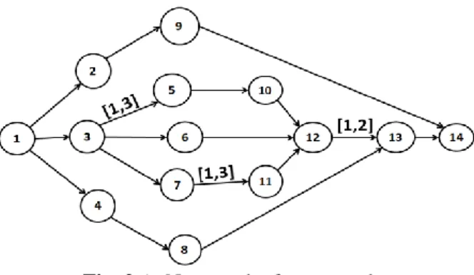
In this section, in order to evaluate and validate the proposed model, it was implemented on synthesized examples. The size of problem rely on the number of activities, number of precedence relations, and number of renewable resources required for the execution of activities. Figure 2 shows the structure of an example. This example has been drawn as AoN network and represents a project with 14 activities (where
51
nodes indicate activities and arcs refer to precedence relations between activities). Activities 1 and 14 are dummy activities with zero duration and zero resource requirements, expressing start and finish activities of the project, respectively.
Fig. 2 AoN network of an example
The values presented over some arcs denote the required time lags for starting the successor activity at the end of the arc, following the completion of the predecessor activity at the start of the arc. Indeed, the lower and upper bounds of the written intervals indicate the minimum and maximum required time following the completion of the predecessor activity before the successor activity can be started; i.e. one should select an integer value from the interval, after which value of time passed following the completion of the precedent activity, the successor activity is to be started. Such a selection process depends on the type of objective function. For example, if the problem objective is solely to minimize total project time, the lower bound of the allowed interval for lag should be chosen. For instance, the interval [1, 2] on the arc linking (precedence relationship) the activity 12 to the activity 13 expresses that, if in a selected sequence, activity 13 is to immediately launched after activity 12 with no activity in-between, 1 or 2 time units must be spent following the completion of activity 12 before activity 13 can be started. Detailed information on this example is reported in table 2.
Table 2. Information on the example
Cash flow Usage Resource2 Usage Resource1 Duration Activity 0 0 0 0 1 -50 15 7 (5,6,7) 2 200 8 1 (4,5,6,8) 3 -30 8 5 (2,3,5) 4 -100 15 6 1 5 20 13 1 (2,3,4) 6 -10 16 2 (1,2,3,4) 7 70 9 2 1 8 100 12 8 (2,4,6) 9 20 17 6 (2,3,5) 10 -50 10 2 1 11 50 5 6 (2,3,4) 12 -100 10 8 (3,5,7) 13 100 0 0 0 14
In this table, activity durations are considered to be various numbers including determined components along with triangular and trapezoidal fuzzy ones. In addition, resources 1 and 2 are renewable with their capacities being 10 and 20 units, respectively.
52
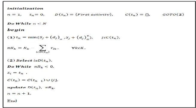
The presented algorithm in figure 3 was applied to obtain allowed domain for the starting time of each activity. If the start times of activities are determined, then we obtain the schedule. Various components of the algorithm are described as follows:
n = 1, … , N Number of steps in which all activities are planned
(dj)α
− Lower bound of α-cut of duration of the
ith activity
(dj)α
+ Upper bound of α-cut of duration of the ith activity πRk Remaining capacity of the kth renewable resource Rk Capacity of the kth renewable resource
rik The renewable resource requirement of activity i for resource k Si Start time of the ith activity
Pi Set of preceding activities of the ith activity C(t̃n) Set of activities scheduled by the time t̃n
D(t̃n) Set of activities not scheduled, but all of their predecessors are completed, by the
time t̃n
Beginning with the algorithm, the first activity, based on selected sequence, is fed into the process. The start time of this activity is set to zero, with the required resources for this activity to execute subtracted from total available resources. In the next step, the second activity comes into play. It also starts at zero time provided the remaining resources are sufficient to have it executed; otherwise, the second activity is delayed until the first activity comes to completion. Due to uncertain nature of the required time to have the first activity finished, its precise time of completion remains undetermined. However, following α-cut approach, one can obtain an interval within which the activity is most likely to be accomplished. At any integer value from this interval, the first activity can be taken as terminates, with the second activity started accordingly. This process continues until corresponding start times for all activities are determined.
Fig 3. Theapplied algorithm to determine domain of starting times of activities within each sequence
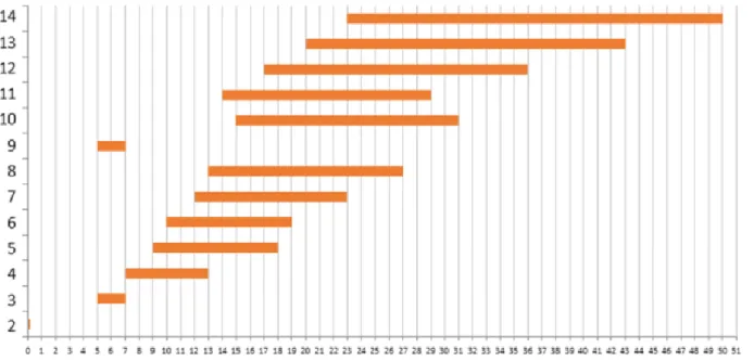
The obtained results for starting times of all activities are shown in figure 4. Note that, the smallest time unit in this study is day, so that, total time of project completion is expressed in days. Hence, out of
53
continuous intervals created by α-cut for fuzzy durations of activities, only integer values rendered acceptable.
Fig 4. Starting times of activities of the example
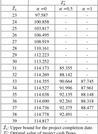
In figure 4, the horizontal axis represents the days past the project start time, while the vertical axis indicates different activities. As the duration of activities is assumed to be integer multiplications of the time unit, among the obtained values for starting times of activities, only integer values can be acceptable. Once allowed values for starting times of all activities were identified, epsilon − constraint method was applied with different values of alpha to establish total domain of starting times for each activity. Obtained using BARON solver in GAMS v.24.2.2, the results are reported in table 3 where the project’s optimum cash flows are obtained for each unit of the upper bound of termination time of the project from 23 to 39 (assuming a discount rate of 0.1).
54
Table 3. Optimal cash flows with bounded termination time for the project
𝑍2∗
𝛼 =1
𝛼 =0.5
𝛼 =0
𝑍̅1 - - 97.587 23 - - 100.858 24 - - 103.817 25 - - 106.495 26 - - 108.919 27 - - 110.161 28 - - 112.223 29 - - 113.252 30 - 85.355 114.173 31 - 88.142 114.269 32 87.745 90.664 114.355 33 87.961 91.996 114.527 34 88.148 92.135 114.638 35 88.318 92.261 114.690 36 88.477 92.375 114.736 37 - 92.491 114.778 38 - - 114.817 39
𝑍̅1: Upper bound for the project completion date.
𝑍2∗: Optimal value of project cash flows.
The blank cells in table 3 refer to failures to find solutions for cash flows considering the corresponding upper bounds and intended α-cut levels. Figure 5 demonstrates the obtained solutions by epsilon − constraint method, with α-cut level considered to be zero, where solid points present obtained Pareto sets of solutions. The horizontal and vertical axes in this diagram indicate the project completion date and NPV of the project's cash flows, respectively.
Fig 5. Pareto solutions for alpha = zero
From table 3 and figure 5, it is evident that, at any specified level of alpha, the NPV of the project cash flows increases with the project duration. That is, the farther the first objective (minimizing total project time) gets from optimal conditions, the closer the second objective (maximizing NPV) gets to optimal
96 98 100 102 104 106 108 110 112 114 116
55
point. Regarding different levels of alpha, it can be expressed that, the higher the alpha level (i.e. the higher the acceptable level of risk by the project manager), the lower the number of Pareto solutions; this is because of smaller intervals created by α-cut over fuzzy activity times, decreasing possible values for starting times of activities.
5- NSGA-II algorithm
When problem is of multi-objective nature, it may be case that no single solution can simultaneously optimize all objectives, so that solving algorithms present solutions on or close to optimum Pareto front, which are nevertheless of high practical value. In fact, the issue with multi-objective optimization is the sorting of solutions – the issue to be resolved by a non-dominated sorting genetic algorithm (NSGA). This algorithm employs a number of criteria to transform not-sorted domain of multi-objective optimization into a sorted domain. This algorithm is associated with some pitfalls, indeed. Deb et al. (2002) developed a mechanism wherein not only solution quality, but also diversity of optimal Pareto solutions were accounted for. Being very effective in the field of multi-objective optimization problems, this method is known as the second version of NGSA: NSGA-II.
Previous researches, as mentioned in section 2.2, prove the superiority of NSGA-II. This method, compared with similar techniques, has lower probability to be trapped in local optimum.The ability of NSGA-II to reach near-optimum solutions has increased its application in large problems. Also, nature of multi-objective resource-constrained project scheduling problem matches with NSGA-II, so this metheuristic algorithm is used to solve this problem. Those are why this algorithm is chosen from a pool of different solving approaches.
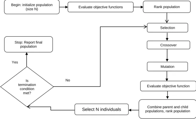
This algorithm addresses the solutions on the basis of two main criteria: quality of solutions and diversity of solutions. With its operators, this algorithm primarily seeks for solutions of the highest quality; however, in case where two (or more) solutions exhibit the same highest quality, the algorithm goes for solutions with larger diversity than the others. A step-by-step flowchart for the NSGA-II algorithm is shown in figure 6.
Fig 6. Flowchart of NSGA-II algorithm
Begin: initialize population
(size N) Evaluate objective functions
Selection
Crossover
Mutation
Evaluate objective function Is
termination condition
met? Yes
No
Rank population
Combine parent and child populations, rank population
Select N individuals
Stop: Report final population
56
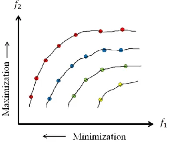
The algorithm proceeds in two main phases. The first phase addresses the quality of solutions, with the second phase addressing their diversities. The first phase sorts the solutions, identifying different fronts, as shown in Fig. 7. For this purpose, the value of two parameters are calculated, namely the number of times a solution dominated, and set of solutions been dominated by the intended solution.
Fig 7. Different solution fronts
In the second phase the crowding distance indicator is applied for expressing the distance among all coplanar solutions (the solutions in one front). The longer the crowding distance of neighboring solutions to a given solution (i.e. the further the solution falls within less populated areas), the larger this point contributes into diversity. Figure 8 represents the crowding distance indicator for the hypothetical solution x placed on the first front.
Fig 8. Crowding distance
When two solutions are compared, two outcomes are possible. First, of two solutions with different ranks, the solution with lower rank is chosen. Second, comparing two solutions on the same front, the one at further crowding distance is selected.
57
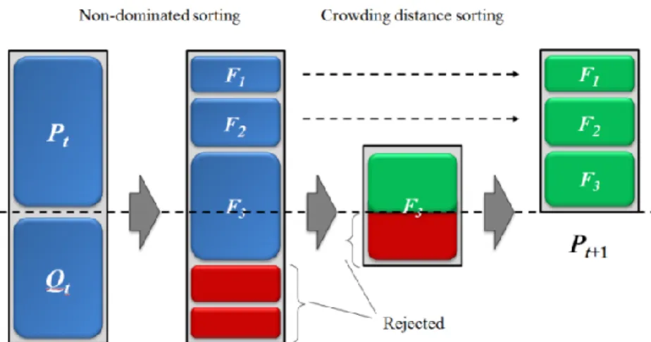
In NSGA-II algorithm, denoting the population of present generation and offspring generated by crossover and mutation operators by Pt and Qt, respectively, the next generation, Pt+1, is developed by,
first, merging Pt with Qt. The merged population is subsequently sorted. Finally, of all solutions currently
available in the set, the same number of solutions in the initial population is directly transferred into the next generation, with the rest of solutions removed. Figure 9 provides an overview of the approach via which the next generation is generated in NSGA-II algorithm.
Fig 9. General mechanism of NSGA-II algorithm in terms of generating the next generation
5-1- Solution encoding
The first step in developing a genetic algorithm is to fit the problem considered into the genetic algorithm structure; i.e. to create a communication bridge between the problem and solution environment before undertaking the evolution process. With an adequate deal of experience and knowledge on the intended problem, one can select an appropriately proportional solution representation to the problem circumstances. This step is one of the most important parts of the algorithm design.
In a RCPSP, the objective is to determine a schedule of activities, considering precedence relations and resource constraints, in such a way to minimize the project completion time. Accordingly, one should form a solution representation to present the priority and sequence of activities. The most appropriate kind of solution representation is an integer solution representation where a chromosome encompasses a set of integer numbers (gens) with their counts being equal to the number of project activities; each integer number is the identification number of the corresponding activity, with resources utilization priority being determined from left to right. Fig. 10 indicates a presentation of a solution for a problem with eight activities, where the activity 4 is prioritized to be the third activity to be executed.
Fig 10. Chromosome structure (activity list)
In the discussed problem in the present study, however, the aim is not only to minimize the project completion time, but also to maximize the net present value of cash flows; i.e. the problem is of multi-objective nature. Here, the two multi-objectives conflict one another, so that, in order to obtain the sequence which can minimize the project duration, one should ignore the second objective, and vice versa. In fact, the minimum time to complete the project is not necessarily associated with optimum cash flow and only when there exists a huge cash inflow for final activity of the project (the project completion), both objectives may deem to act along the same direction (i.e. the minimum project duration creates the maximum NPV). On the other hand, uncertainties in activity times and using fuzzy numbers to express these uncertainties lead starting times of activities to be undetermined in an assumed sequence. However,
58
by converting fuzzy numbers into crisp numbers, one can obtain total domain or set of possible values for starting times of activities in any selected sequence. Using this domain, one can determine starting times, improving the second objective (i.e. to maximize NPV) by examining the starting point of each activity according to the allowed domain of starting times, so as to obtain Pareto solutions. Using the algorithm described in Section 4, all possible dates of starting different activities are obtained for any of the created sequences. Therefore, each chromosome must contain information on starting times of activities. Furthermore, the intended chromosome not only contains starting times of activities, includes associated information with time lags. This means that, if, in a created sequence, two activities, with their precedence relation considered to involve a time lag, are planned to launch immediately following one another, the time lag is to be applied, so that, one should select an integer time lag value from the allowed range after which time lag past the termination of the predecessor activity, the successor activity can be started.
5-2- Fitness function
Different solutions are compared to one another and sorted based on the calculation of objective functions. In fact, based on domination law, a solution is preferable over another one if it is not worse than that when any of the objectives are concerned (completion time minimization and cash flow maximization), while being better in at least one of the objectives. For any given solution, completion time refers to the starting time of the final dummy activity, with the project cash flow NPV obtained by calculating sum of associated cash flows with all of activities at their starting times, considering the discount rate.
5-3- Crossover operator
Being a process where a new offspring solution is created by combining two parent solutions, crossover is the important feature of genetic algorithm, so that many researches have considered it as the main mechanism for promoting diversity. The aim of combining two parent chromosomes is to achieve a better chromosome, as parts of features in parent chromosomes transfer to the offspring.
Crossover operator is dependent on the solution representation, so that different operators should be applied for different solution representations. For the intended chromosomes, several crossover operators have been developed, among which the two most commonly used ones are employed in this study.
5-3-1- UX3 crossover
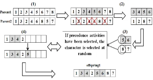
The UX3 crossover is used for chromosomes related to activity sequencing and prioritizing. The highlighted features of this type of crossover which have made it suitable for activity prioritizing tasks are that, it prevents from repeating each activity along the length of chromosome while considering the precedence relations between activities. The UX3 crossover operator performs the chromosome crossover by creating two exclusive substrings from parent strings and then randomly writing the characters in the created substrings to the offspring strings. While the characters are being written into the offspring strings, activity precedence relations are also taken into account. The procedure of UX3 is performed as follows: Step 1: two positions are randomly selected along the first string (i.e., Parent 1),
Step 2: considering the substring defined by the two positions from Parent 1, the characters already existing in substring are deleted from Parent 2.
Step 3: considering activity precedence relations, characters from the two substrings are randomly selected. If precedence activities of a selected activity are not selected yet, then the character selection is skipping.
Step 4: the characters are placed, from left to right, into unfixed positions of an offspring string.
Step 5: Steps 3 and 4 are repeated until the offspring chromosome is completed. Following similar approach, the second offspring is produced from the same parents.
59
Fig 11. Operation of UX3 crossover
5-3-2- Cyclic crossover
Another crossover operator used to prioritize different activities is cyclic crossover operator. This working mechanism of this operator begins with selecting a random number point across which the parent chromosomes will be cut, dividing them to two substrings. Accordingly, initially created substring from the first parent forms initial part of the first child. Then, the existing gens in this substring are removed from the second parent, with its remaining gens (with their sequence) forming the second part of the first child.
In order to create the second child, the same process is undertaken with the first and second parents replaced, i.e. the initial substring for the initial part of the second child is taken from the second parent and so on.
Figure 12 shows how this operator works for an example with 8 activities.
Fig 2. Operation of cyclic crossover
5-4- Mutation operator
Mutation refers to a genetic phenomenon rarely occurring in some chromosomes via which offspring gains features that belong to none of its parents. The mutation operator follows a random approach with its aim being to search more points across the solution space, so as to avoid early convergence. In mutation, a number of gens are randomly selected and their integer values are changed. Similar to crossover operator, mutation depends on solution representation, so that different mutation operators are
60
applied for different solution representations. In the following two types of applicable mutation operators are described for the intended chromosomes.
5-4-1- UM3 mutation
Being specific to activity prioritization chromosomes, this type of mutation ensures no repeated activity along the string while considering precedence relations between activities, in the course of mutation operation. The basics of UM3 mutation operator is similar to those of UX3 crossover, except for that, character alteration is undertaken within an individual chromosome. Accordingly, first, a substring is selected from a parent chromosome. Then, the characters in the substring are exchanged at random. When exchanging the characters, activity precedence relations are also taken into account. Continuing with the operation, the new substring is put back into the parent string in the same position to obtain an offspring chromosome for the next generation.
Figure 13 demonstrates how this operator works.
Fig 3. Operation of UM3 mutation
5-4-2- Random relocation mutation
This operator is only applied to chromosomes wherein the gens are integer numbers. In order to use this operator, it is necessary to define a real parameter, 𝛾, ranging from 0 to 1, so that, by multiplying this parameter by the number of gens in a chromosome and rounding up the result, one can end up with the number of gens to be selected randomly and moved along the length of the chromosome. Fig. 14 shows how random relocation mutation operator works.
61
5-5- Operator selection mechanism
A roulette wheel-based approach is used to select from mentioned crossover and mutation operators. For crossover operation, for example, the probability of choosing UX3 crossover operator is denoted by PrUX3, with that of cyclic cross over referred to by PrCC (where PrCC = 1-PrUX3); subsequently, roulette wheel approach - that follows a uniform probability distribution - is used to select the intended crossover operator. The same process is applied to mutation operators, so that, probabilities of selecting UM3 and random relocation mutation operators are denoted by PrUM3 and PrRRM, respectively.
Naturally, at any round of iteration along the algorithm, the method with higher probability is more likely to be selected by the roulette wheel. Also, as finding probabilities for each crossover and mutation approach plays a significant role in this regard, assigning optimal probability values may contribute to desirable solutions.
5-6- Parents selection mechanism
To select parents for crossover and mutation operations, binary tournament selection is used where chromosomes are compared to one another in a pairwise manner, and then ranked. Accordingly, the lower the rank, the superior the chromosome, i.e. the chromosome of the lower rank is selected. In cases where both chromosomes exhibit the same rank, the second criterion comes into play: crowding distance – the further the crowding distance, the superior the chromosome.
5-7- Initial population generation
Initial population refers to the initial set of chromosomes. Each chromosome represents a point in solution space of the problem, and so, the purpose of generating an initial population is to create a number of solutions for the problem. The genetic algorithm then starts with generating an initial population of chromosomes which is fed into the problem as an adjustable parameter. At the beginning, an initial population is randomly created; however, applying different operators of genetic algorithm, the next generations are generated.
5-8- Termination condition
Since genetic algorithm is a meta-heuristic approach working on the basis of solution generation and testing, the developed solutions may not be well-specified i.e. it is not determined which exact solution represents optimal solution, so as to define termination criterion based on finding the optimal solution. For this reason, other termination criterion was introduced into the proposed algorithm: number of iterations (number of times the main loop of the program was launched). Therefore, following a predefined number of iterations of the main loop, the program came to stop with the obtained solutions reported.
6- Computational results
6-1- Creating synthetic samples
In order to test the presented algorithm, a number of standard samples were used. With no relevant samples in related literatures, some samples of different sizes are synthesized in this section. The samples are acceptable from the perspective of logic of diagram, with their cash flows and activity times being logical and fully explainable. Each sample is taken from a different authentic reference with the missing required information addressed by introducing logical information aligned with the existing information. The samples were classified based on dimension and size, so that the samples with less than 10 activities were classed under small-scale problems, those with 10 to 30 activities were classed under medium-scale problems, and those with more than 30 activities were grouped into large-scale problems.
6-2- Adjustment of parameters
Meta-heuristic algorithms are sensitive to their parameters, such that a small change in parameters can considerably affect their performance. In general, the algorithm parameters include crossover rate,
62
mutation rate, and population size of any generation; these can strongly affect convergence behavior as well as quality and diversity of solutions.
In the proposed algorithm, other parameters such as number of iterations of the main loop, number of random selections from obtained values for starting times, probability of using various crossover and mutation operators, and used rate for random relocation mutation are added to the program. Once adjusted, these can enhance the algorithm performance to obtain better solutions.
The proposed algorithm was coded in MATLAB. Table 4 indicates parameter values as adjusted for the NSGA-II algorithm for problems of different sizes. In this table, n expresses the number of activities in respective problem. Parameters were adjusted according to sensitivity analysis where, keeping all other parameters constant, the increase in the number of non-dominated solutions by increasing each of the parameters was calculated, so as to increase the value of the parameter with the largest contribution into increased number of non-dominated solutions.
Table 4. Proposed values for parameter adjustment
Proposed values Adjustable parameters Large-scale problems Medium-scale problems Small-scale problems 3n 3n 4n Population size 10 20 40 Maximum number
of iterations of the main loop
5 20
10 Number of random
selection from starting times 0.4 0.5 0.7 Crossover rate 0.1 0.1 0.3 Mutation rate 0.5 0.5 0.5 Probability of UX3
crossover 0.5 0.5 0.5 Probability of cyclic crossover 0.5 0.5 0.5 Probability of UM3
mutation 0.5 0.5 0.5 Probability of random relocation mutation 0.01 0.01 0.01 Rate of random
relocation mutation
6-3- Validation of the proposed algorithm
The NSGA-II algorithm is likely to present logical and acceptable solutions if its components (e.g. initial population generation, crossover and mutation operators, etc.) are defined appropriately. Furthermore, to have the algorithm results closer to the Pareto front and also to have solution more appropriately distributed, performances of applied approaches in the algorithm components and validity of solutions must be evaluated. In table 5, three sample problems of different sizes are compared based on the number of obtained non-dominated solutions from the algorithm at different levels of alpha and execution time of the algorithm.
63
Table 5. The algorithm results for three different sample problems.
CPU time(s) Number of non-dominated
solutions Nu m b er o f ren ewa b le reso u rce s Nu m b er o f ac tiv ities Alpha 1 0.8 0.6 0.4 0.2 0 33 5 6 8 9 11 12 3 7 38 4 5 7 9 9 10 2 14 52 3 5 6 7 8 9 2 31
6-4- Evaluation criteria
Due to complexity of the raised problem, it cannot be solved by classic methods, so, generally, obtaining optimal Pareto solutions and comparing them with those returned by the algorithm is not an option. Alternatively, the relevance and quality of solutions of the proposed algorithm are assessed in terms of the following indicators and criteria:
Maximum spread (MS)
Generational distance (GD) Spacing metric (SM) Mean ideal distance (MID)
6-5- Computational results
In order to evaluate the algorithm in terms of the above criteria, the results of sample problems with different sizes are investigated.
6-5-1- Small-scale problems
Table 6 presents the solution of a small-scale sample problem as obtained from execution of the algorithm. In figure 15, the algorithm solutions are compared against exact solutions.
64
Table 6. Non-dominated solutions of a small-scale sample problem for alpha = zero
𝑍2
𝑍1
Starting times of activities Created sequences No n -d o m in ated so lu tio n s 78.830 25 [0,0,0,0,17,22,25] [1,2,4,3,6,5,7] 1 79.728 26 [0,0,0,0,17,23,26] [1,2,4,3,6,5,7] 2 82.462 27 [0,0,0,0,16,24,27] [1,2,4,3,6,5,7] 3 85.881 30 [0,0,0,0,15,26,30] [1,2,4,3,6,5,7] 4 106.944 35 [0,0,0,10,19,30,35] [1,2,4,5,3,6,7] 5 108.024 36 [0,0,0,11,17,29,36] [1,2,4,5,3,6,7] 6 111.227 37 [0,0,0,12,18,32,37] [1,2,4,5,3,6,7] 7 116.209 39 [0,0,0,14,18,33,39] [1,4,2,5,3,6,7] 8 127.060 40 [0,0,0,18,21,35,40] [1,2,4,5,3,6,7] 9 131.434 45 [0,0,0,21,25,39,45] [1,2,4,5,3,6,7] 10 134.554 49 [0,0,0,21,28,42,49] [1,2,4,5,3,6,7] 11 135.143 50 [0,0,0,20,29,44,50] [1,2,4,5,3,6,7] 12
Fig 55. A comparison between the algorithm solutions and exact solutions of a small-scale sample problem for alpha = zero
It is worth noting that, due to very small size of this sample problem, all of its possible sequences were surveyed and the exact solution was obtained, which, in general, is extremely difficult (almost impractical) to undertake for problems of average size.
65
6-5-2- Medium-scale problems
Table 7 shows the solutions of a medium-scale sample problem as obtained in a singly run of the algorithm. Fig. 16 presents the results of solving the problem by the algorithm at different levels.
Table 7. Non-dominated solutions of a medium-scale sample problem for alpha = zero
Difference percentage (errors) Exact values
of 𝑍2
Obtained values for 𝑍2
𝑍1 No n -d o m in ated so lu tio n s 3.74 202.050 194.502 27 1 0.04 206.363 206.281 28 2 1.24 218.797 216.086 30 3 0.05 217.896 217.782 32 4 0 218.061 218.061 33 5 1.35 222.361 219.360 34 6 1.15 223.132 220.561 37 7 1.25 223.650 220.859 39 8 0.87 223.863 221.916 40 9 0.48 223.044 221.963 42 10 0.03 223.278 223.205 43 11
Fig 16. Solutions of a medium-scale sample problem as obtained by the algorithm at different levels of alpha
6-5-3- Large-scale problems
Table 8 indicates the solutions of a large-scale sample problem as obtained from execution of the algorithm, while figure 17 demonstrates the results of solving the problem by the algorithm at different levels.
66
Table 8. Non-dominated solutions of a large-scale sample problem for alpha = zero
Difference percentage (errors) Exact
values of 𝑍2
Obtained values for 𝑍2 𝑍1 No n -d o m in ated so lu ti o n s 0.31 116.344 115.985 136 1 2.65 121.101 117.896 138 2 6.26 129.832 121.707 141 3 0 141.596 141.596 142 4 0.38 144.145 143.592 144 5 0.08 147.862 147.740 146 6 0.07 149.416 149.316 151 7 0.1 150.002 149.844 153 8 0.02 152.343 152.312 155 9 1.74 155.060 152.356 167 10
Fig 6. Solutions of a large-scale sample problem as obtained by the algorithm at different levels of alpha
6-5-4- Algorithm performance for problems with different sizes
Last but not the least; a comparison was made on the algorithm performance when dealing with problems of different scales. As dimensions of a problem increase, algorithm presents lower number of non-dominated solutions. However, when it comes to other evaluation criteria, one cannot provide a precise opinion. As such, comparing five sample problems of different sizes, one can end up with a more realistic and logical insight. Figure 18 shows the results of solving problems of different sizes by the algorithm.
67
Fig 78. The algorithm-obtained solutions for problems of different sizes for alpha = zero
As can be noticed from the figure, considering different criteria, the algorithm exhibits its highest performance in small-scale problems, and as problem dimensions increase, its performance decreases.
7- Conclusion
Scheduling problem is one of prominent and pervasive problems in the field of project control and management. Project scheduling is aimed at determining optimal project duration, and in case where the intended project is recourse-constrained, the objective is to determine optimum sequence of activities considering precedence relations and constraints in resources, so as to obtain minimum required time to bring the project to completion. In order to further account for economic aspects, it is necessary to add another objective to the problem to consider the project cash flows. Using fuzzy numbers to express uncertainties in activity times, not only brings the problem closer to real world, but also highly diversifies the solution set. Other concepts introduced to further adapt the problem to real world cases include multi-resource problem environment, and time lags in precedence relations between activities.
Resource-constrained project scheduling problems are NP-Hard, so that the required time to have them solved increases, exponentially, with increasing the problem dimensions. On the other hand, the assumptions taken in the present study further increased the problem complexity. Therefore, to achieve desirable solutions within an acceptable time span, it is necessary to employ meta-heuristic approaches. As a suggestion for future studies, uncertainties in other parameters of problem can be considered following a fuzzy logic approach. Moreover, one can use other meta-heuristic algorithms to solve the discussed problems.
68
References
Abello, M. B., & Michalewicz, Z.(2014). Multiobjective resource-constrained project scheduling with a time-varying number of tasks, The scientific world journal, Volume 2014, Article ID 420101.
Agarwal, R., Tiwari, M., & Mukherjee, S.(2007). Artificial immune system based approach for solving resource constraint project scheduling problem, The International Journal of Advanced Manufacturing Technology, 34, 584-593.
Artigues, C., Leus, R., Nobibon, F. , (2015). The stochastic time-constrained net present value problem, In: Schwindt, C., Zimmermann, J., editors. Handbook on Project Management and Scheduling Vol. 2. Springer, 875-908.
Atli, O. , & Kahraman, C.(2014). Resource-constrained project scheduling problem with multiple execution modes and fuzzy/crisp activity durations, Journal of Intelligent & Fuzzy Systems: Applications in Engineering and Technology, 26, 2001-2020.
Ballestín, F. (2007, April). A genetic algorithm for the resource renting problem with minimum and maximum time lags. In European Conference on Evolutionary Computation in Combinatorial Optimization (pp. 25-35). Springer Berlin Heidelberg.
Bartusch, M., Möhring, R. H., & Radermacher, F. J.(1988). Scheduling project networks with resource constraints and time windows, Annals of Operations Research, 16, 199-240.
Berthaut, F., Pellerin, R., Perrier, N. & Hajji, A.(2014). Time-cost trade-offs in resource-constraint project scheduling problems with overlapping modes. International Journal of Project Organisation and Management,6,215-236.
Čapek, R., Šůcha, P., & Hanzálek, Z. (2012). Production scheduling with alternative process plans. EuropeanJournal of Operational Research, 217(2), 300-311.
Chanas, S., & Zieliński, P.(2001).Critical path analysis in the network with fuzzy activity times, Fuzzy sets and systems, 122, 195-204.
Chassiakos, A. P., & Sakellaropoulos, S. P.(2005). Time-cost optimization of construction projects with generalized activity constraints, Journal of Construction Engineering and Management, 131, 1115-1124. Davis, K. R., Stam, A., & Grzybowski, R. A.(1992). Resource constrained project scheduling with multiple objectives: A decision support approach, Computers & Operations Research, 19, 657-669. De Reyck, B., & Herroelen, W.(1998). An optimal procedure for the resource-constrained project scheduling problem with discounted cash flows and generalized precedence relations, Computers & Operations Research, 25, 1-17.
Deb, K., Pratap, A. , Agarwal, S., & Meyarivan, T.(2002). A fast and elitist multiobjective genetic algorithm: NSGA-II, IEEE Transactions on Evolutionary Computation, 6, 182-197.
Demeulemeester, E. L., & Herroelen, W. S.(1996). Modelling setup times, process batches and transfer batches using activity network logic, European Journal of Operational Research, 89, 355-365.
69
Drexl, A., Nissen, R., Patterson, J. H., & Salewski, F. (2000). ProGen/πx–An instance generator for resource-constrained project scheduling problems with partially renewable resources and further extensions, European Journal of Operational Research, 125, 59-72.
Dubois, D. J.(1980). Fuzzy sets and systems: theory and applications vol. 144. Toulouse, France: Academic press.
Elloumi, S., Fortemps, P., & Loukil T.(2017). Multi-objective algorithms to multi-mode resource-constrained projects under mode change disruption. Computers & Industrial Engineeirg, 106, 161-173. Ghamginzadeh, A., Najafi, A.A., & Azimi, P.(2014). Solving a multi-objective resource-constrained project scheduling problem using a cuckoo optimization algorithm, Scientia Iranica, 21(6), 2419-2428. Gomes, H.C., Neves, F.A., Souza, M.J.F. (2014). Multi-objective metaheuristic algorithms for the resource-constrained project scheduling problem with precedence relations. Computers &Operations Research, 44, 92-104.
Habibi, F., Barzinpour, F., Sadjadi, S.J. (2017). A Multi-objective optimization model for project scheduling with time-varying resource requirements and capacities. Journal of Industrial and System Engineering, 10, 92-118.
Hao, X., Lin, L., & Gen, M. (2014). An effective multi-objective EDA for robust resource constrained project scheduling with uncertain durations. Procedia Computer Science, 36 , 571-578.
Hapke, M., & Slowinski, R.(1996). Fuzzy priority heuristics for project scheduling, Fuzzy sets and systems, 83, 291-299.
Hapke, M., Jaszkiewicz, A., & Slowinski, R.(1994). Fuzzy project scheduling system for software development, Fuzzy sets and systems, 67, 101-117.
Hapke, M., Jaszkiewicz, A., & Słowiński, R.(1998). Interactive analysis of multiple-criteria project scheduling problems, European Journal of Operational Research, 107, 315-324.
Herroelen, W., & Leus, R. (2005). Project scheduling under uncertainty: Survey and research potentials. European journal of operational research , 165 (2), 289-306.
Kazemi, F., & Tavakkoli-Moghaddam, R.(2011a). Solving a multi-objective multi-mode resource-constrained project scheduling problem with particle swarm optimization, International Journal of Academic Research, 3, 103-110.
Kazemi, F. , & Tavakkoli-Moghaddam, R.(2011b).Solving a multi-objective multimode resource-constrained project scheduling problem with discounted cash flows, 6th International Project Management Conference, vol. 3.
Khalili, S., Najafi, A. A., & Niaki, S. T. A.(2013). Bi-objective resource constrained project scheduling problem with makespan and net present value criteria: two meta-heuristic algorithms, The International Journal of Advanced Manufacturing Technology, 69, 617-626.
Kolisch, R., & Hartmann, S. (2006). Experimental investigation of heuristics for resource-constrained project scheduling: an update. European Journal of Operational Research, 174, 23–37.
70
Leyman, P. & Vanhoucke, M. (2016). Payment models and net present value optimization for resource- constrained project scheduling. Computers & Industrial Engineering, 91,139-153.
Maghsoudlou, H., Afshar-Nadjafi, B., & Akhavan Niaki, S.T. (2016). A multi-objective invasive weeds optimization algorithm for solving multi-skill resource constrained project scheduling problem. Computers & Chemical Engineering, 88, 157-169.
Mogale, D. G., Kumar, S. K., & Tiwari, M. K. (2016). Two-stage Indian food grain supply chain network transportation-allocation model. IFAC-PapersOnLine, 49(12), 1767-1772.
Mogale, D.G., Kumar, S.K., & Tiwari, M.K. (2018). An MINLP model to support the movement and storage decisions of the Indian food grain supply chain. Control Engineering Practice, 70, 98-113.
Mogale, D.G., Lahoti, G., Jha, S.B., Shukla, M., Kamath, N., & Tiwari, M.K. (2018). Dual market facility network design under bounded rationality. Algorithms, 11(54), 1-18.
Mogale, D.G., Kumar, M., Kumar, S.k., Tiwari, M.K. (2018). Grain silo location-allocation problem with dwell time for optimization of food grain supply chain network. Transportation Research Part E, 111, 40-69.
Moradi, M., Hafezalkotob, A., Ghezavati, V.R. (2018). The resource-constraint project scheduling problem of the project subcontractors in a cooperative environment: Highway construction case study. Journal of Industrial and System Engineering, 11(3). Published Online.
Nahmias, S.(1978). Fuzzy variables, Fuzzy sets and systems, 1, 97-110.
Nudtasomboon, N., & Randhawa, S. U.(1997). Resource-constrained project scheduling with renewable and non-renewable resources and time-resource tradeoffs, Computers & Industrial Engineering, 32, 227-242.
Palacio, J. D. & Larrea, O. L. (2017). A lexicographic approach to the robust resource-constrained project scheduling problem. International Transactions in Operational esearch, 24,143-157.
Tao, S. & Dong, Z.S. (2018). Multi-mode resource-constrained project scheduling problem with alternative project structures. Computers & Industrial Engineering, 125, 333-347.
Tritschler, M., Naber, A., Kolisch, R. (2017). A hybrid metaheuristic for resource-constrained project scheduling with flexible resource profiles. European Journal of Operational Research, 262(1), 262-273. Vanucci, S. C., Bicalho, R., Carrano, E. G., & Takahashi, R. H.(2012). A modified NSGA-II for the Multiobjective Multi-mode Resource-Constrained Project Scheduling Problem, IEEE Congress on Evolutionary Computation (CEC), pp. 1-7.
Wang, L., Zheng, X.-L. (2018). A knowledge-guided multi-objective fruit fly optimization algorithm for the multi-skill resource constrained project scheduling problem. Swarm and Evolutionary Computation, 38, 54-63.
71
Wieseman, W., Kuhn, D., (2015). The stochastic time-constrained net present value problem, In: Schwindt, C., Zimmermann, J., editors. Handbook on Project Management and Scheduling Vol. 2. Springer, 753-780.
Wiest, J. D. (1962). The scheduling of large projects with limited resources, Ph.D. dissertation, DTIC Document.
Xiao, J., Wu, Z., Hong, X. X., Tang, J. C., & Tang , Y. (2016). Integration of electromagnetism with multi-objective evolutionary algorithms for RCPSP. European Journal of Operational Research, 251(1), 22-35.
Zhao, Z. Y., You, W. Y., & Lv, Q. L.(2008). Applications of fuzzy critical chain method in project scheduling, in Natural ComputationI, Fourth International Conference on CNC'08., 473-477.