A chance-constrained multi-objective model for final assembly
scheduling in ATO systems under uncertainty in the subassembly
availabilities
Leila Izadkhah1, M. M. Lotfi1* 1
Department of Industrial Engineering, Faculty of Engineering, Yazd University, Yazd, Iran
[email protected], [email protected]
Abstract
In this paper a chance-constraint multi-objective model under uncertainty in the availability of subassemblies is proposed for scheduling in ATO systems. The on-time delivery of customer orders as well as reducing the company's cost is crucial; therefore, a three-objective model is proposed including the minimization of1) overtime, idletime, change-over, and setup costs, 2) total dispersion of items’ delivery times in customers’ orders, and 3) tardiness and earliness costs.In order to reduce the involved risk, the uncertainty in the subassembly availabilities is addressed via a chance-constrained programming. The lexicographic method is employed to solve the model. The performance and validity is then evaluated using the real data from an electrical company. Notably, the decision maker can draw the appropriate results by a priority establishment between the costs and delivery time objectives. Moreover, formulating the existing uncertainty in the subassembly availabilities helps avoiding delay in the orders’ completion dates. Finally, applying joint lot size policy leads to a more proper scheduling of assembly sequence.
Keywords: Assemble-to-order, final assembly schedule, joint lot size,
chance-constrained programming, multi-objective optimization
1- Introduction
Nowadays, according to the competitive conditions in the manufacturing industries, the assemble-to-order (ATO) systemsprovidinga various line of products with reasonable delivery timesare increasingly taken into account. Previous researchers’ studied ATO system in the industries like electronics and computers (Xiaoet al., 2010). Notably, an ATO strategy is used for the systems in which some types of variation in the final products’ demands exist (Elhafsi& Hamouda, 2015). In this strategy, the components and subassemblies are acquired or manufactured according to the forecasts while the final assembly is not scheduled until the detailed final product specifications are derived from the customer’s order (Wemmerlöv, 1984). Since 1990s, many companies, such as Dell, facing the ever-increasing competition and needing the mass customization, chose to adopt the ATO system in order to increase the product offering and to reduce the product’s life cycles (Wang, 2014).
*Corresponding author
ISSN: 1735-8272, Copyright c 2017 JISE. All rights reserved Journal of Industrial and Systems Engineering
Vol. 10, Special Issue on Scheduling, pp. 1-16 Autumn (November) 2017
Among the various manufacturing strategies, ATO is a popular one as it can reduce the delivery costs with high diversity products. In the ATO systems, fabricating the subassemblies are scheduled via the well-known Master Production Scheduling (MPS) process; then based upon, the assembly of end itemsordered and configured by the customers is conducted througha postponed schedule namely final assembly scheduling (FAS) (Olhager &Wikner, 1998). In fact, a well-established Final Assembly Scheduling (FAS) is an essential tool to reduce the related costs and delivery times of customer’s orders as well as the imposed penalties of earliness and tardiness. Hence, two consecutive schedules are usually needed in the ATO systems: MPS for subassemblies and fabricated components and FAS for the final products.This increases the efficiency of ATO systems and provides a better response to the customers. Despite their popularity, ATO systems are known to be difficult to analyze and manage. In practice, ATO systems are managed using heuristics or other ad hoc procedures whose effectiveness relative to optimal policies remains difficult to verify (El-Hafsi, 2009). ATO environments are often characterized by some significant uncertainty especially in the availability of sub assemblies and fabricated components. Sub assemblies are supplied inside the factory or outside via the suppliers; however, their appropriate quantities cannot certainly be determined for various reasons like incorrect forecasts, failure of equipment, lack of timely delivery from the suppliers and etc. Therefore, receiving the sub assemblies may not be on time and the delivery of orders is faced with tardiness. Firstly, in the most previous researches, the lead time of sub assemblies was considered to be uncertain; but, the more important uncertainty in the quantities of planned subassemblies (i.e., availability) was not addressed. While often, the required amounts of sub assemblies planned through the MPS do not reach in the scheduled time; this causes the incomplete and/or delayed delivery as well as the cost of tardiness. Moreover, the FAS is a multi-objective problem in nature. For instance, theutilization of assembly lines and efficient deliveries are also critical.
One of the most important applications of ATO manufacturing strategy is in electronic, computer and billboard industries. In such industries, the variety of products is high; hence, to improve the response to market requirements as well as to reduce the corresponding costs, they have tended to the ATO systems.This research, inspired by the scheduling problem of an electrical company,is conducted to make the more effective scheduling for such industries. In this paper, thus, supposing a given MPS at hand, a chance-constrained multi-objective FAS optimization in ATO systems is proposed for a cost-efficient and timely delivery of the customer’s orders. Due to the above-mentioned uncertainties originating from the internal and/or external environment which cause the random deviations of the actual available sub assemblies from the MPS quantities, we employ a chance-constraint in the proposed FAS model. Three objectives including the minimization of capacity-related costs, sum of the completion time dispersions for customer’s orders, and tardiness/earliness penalties. We implement our model for a real case of a panel manufacturing factory.
The rest of the paper is organized as follows. Section 2 elaborates the relevantresearch onthe scheduling in ATO systems. In section 3, the proposed model is presented and discussed.Analytical results for the case study are given in section 4. We conclude the advantages of the proposed model and future research directions in section 5.
2- Literature review
ATO systems have significantly been studied in the literature since 1980s. Two major researches are conducted on the analysis of performance measures (e.g., the optimal inventory policies) under the different environments, and understanding the impacts of alternative system designs (Xiao et al., 2010).The problems under investigation comprisedof the single or multiple products as well asthe single or multiple periods.
Among the issues related to the inventory management of components and sub assemblies in ATO systems, multi-stage optimal lot-sizing problems are extremely intractable. Chiu & Lin (1988) considered the case of one finished product. Applying the concepts of echelon stock and topology structure, they obtained the optimal solutions of multi-stage/series assembly systems by a dynamic programming algorithm. Song et al. (2002) studied a product due date assignment procedure developed for complex products with many stages of manufacturing and assembly in conditions of uncertainty in processing time. The proposed method systematically decomposed the complex product
structures of multistage assemblies into the two-stage sub systems. Chang et al. (2012) formulated a two-stage assembly system with imperfect processes, independent component processes, and variable assembly rates as a cost minimization model. Karaarslan et al. (2013) studied the inventory management and supply planning in an ATO system with one product and two sub assemblies each of which had the different review period. Their results suggested that the balanced base stock policy works better than the pure base stock policy under low service levels. Horn & Lin (2016) formulated a stochastic simulation optimization problem and a metaheuristic solution algorithm for an ATO system operating under a continuous-review base-stock policy. They applied it to a large system with 12 items on eight products.
The previous researches on the ATO systems considered the uncertainty in the parameters including lead times, demands and capacity.Yano (1987) studied the stochastic lead times in the two-level assembly systems with the objective of minimizing the sum of inventory holding costs and tardiness costs. Kumar (1989) studies the expected inventory holding time for each component in an ATO environment where the demand was known and there were fixed due dates; but the component procurement lead times were random. Chu et al. (1993) proposed a single-period model for the optimal values of planned lead times in a one-level assembly system with an arbitrary number of component types, fixed punctual finished product demands and random component procurement times. Dolgui et al. (1996) proposed a multi-product multi-period discrete model for the assembly planning under constant demand and random component procurement times for the lot-for-lot policy. They took the item holding and finished product backlogging costs into account. The approach was based on the coupling of an integer linear programming and simulation models. Proth et al. (1997) proposed a model for the supply and assembly planning under the constant demand for finished productsand random delivery times of the items for assembly. They determined the production scheduling according to a fixed policy.
Dolgui & Ould-Louly (2002) proposed a model for supply planning under lead time uncertainty which minimized the expected backlogging and holding costs. Tang et al. (2003) studied a two component assembly system with stochastic lead times (for components) and fixed finished product demand for a known due date. The objective was to minimize the total stock out and inventory holding costs. The Laplace transform procedure was used to capture the stochastic properties of lead times. Axsater (2005) considered a multi-level assembly system with operation times as independent random variables. The objective was to minimize the sum of expected holding and backlogging costs; an approximate decomposition technique was proposed. Hnaien et al. (2009) studied the supply planning for two-level assembly systems under lead time uncertainties. Considering the summation of holding and stock-out costs as the objective, they used genetic algorithm to solve the problem. In Hnaien et al. (2010), the same problem was studied with the objectives of minimizing the holding costs and the stock-out probability; two multi-objective genetic algorithms were applied to solve the problem.
In some researches, the uncertainty in the demands of finial products was considered. Gurnani et al. (1996) considered a problem with two components assuming that the components arrive in either the current or the next periods with given probabilities and the demands for final product were stochastic. The model optimized the orderquantity of each item for each supplier. De Croix et al. (2009) considered a multi-product ATO system; in addition to the stochastic demand for the final products, the system experienced the stochastic returns of subsets of components which can then be used to satisfy the subsequent demands. They presented a heuristic method for computing a base-stock policy. Cheng et al. (2011) studied the optimal production and inventory allocation of a single-product ATO system with multiple demand classes and lost sales. They used an exponential distribution to approximate the distribution of the total processing times and proposed two heuristic policies to address the problem. Elhafsi & Hamouda (2015) considered an ATO manufacturing system producing a single product assembled from some components, and serving an after sales market for individual components. The demands for the product occurred according to the independent Poisson streams. Production times were exponentially distributed with finite production rates. Components were produced in a make-to-stock fashion. In order to characterize the optimal production and inventory rationing policies, they formulated the problem as a Markov decision process.Wang et al. (2017) developed a multi-objective model and hybrid artificial bee colony algorithm for order scheduling and mixed-model sequencing in ATO systems in order to maximize net profits, minimize change-over times and level material usage.Table 1 provides a literature summary in terms of model description, involved uncertainty,
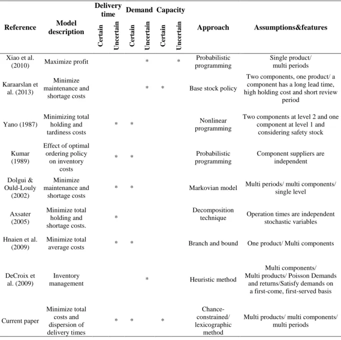
approach, assumptions and features. Most of the previous studies in the ATO systems focused on the inventory management for sub assemblies to reduce their costs, while they did not consider the uncertainty in the availability of sub assemblies. In reality, the available amounts of sub assemblies in each period faced uncertainty due to the existing internal/external uncertainties. Moreover, the literature mainly considered stock-out and carrying costs as the objective, while the capacity-related costs (i.e., those of idle time, over time, setup and change-over) as well as the efficient order deliveries are also of similar importance for decisions. Hence, in this paper, we develop a chance-constrained multi-objective optimization model for FAS in ATO systems taking the uncertainty in the availability of sub assemblies into consideration. In the first objective (i.e., minimization of capacity-related costs), we aim at improving the capacity utilization of the assembly lines. A customer may have several final product models in her order portfolio; hence, in order to deliver the order portfolio on time, all the corresponding final product models should be completed nearly. In the second objective (i.e., minimizing the sum of the completion time dispersions of final product models in the customers’ orders) we purpose to have efficient deliveries. In the third objective (i.e., minimization of tardiness/earliness penalties), the carrying and stock-out costs are tried to be addressed. Note worthily, no restriction in the type and number of sub assemblies and final products as well as the number of periods is imposed.
Table 1. Literature summary
Assumptions&features Approach Capacity Demand Delivery time Model description Reference U n ce rt a in C er ta in U n ce rt a in C er ta in U n ce rt a in C er ta in Single product/ multi periods Probabilistic programming * * Maximize profit
Xiao et al. (2010)
Two components, one product/ a component has a long lead time, high holding cost and short review
period Base stock policy
* * Minimize maintenance and shortage costs Karaarslan et al. (2013)
Two components at level 2 and one component at level 1 and
considering safety stock Nonlinear programming * * Minimizing total holding and tardiness costs Yano (1987)
Component suppliers are independent Probabilistic
programming *
* Effect of optimal
ordering policy on inventory
costs Kumar
(1989)
Multi periods/ multi components/ single level Markovian model * * Minimize maintenance and shortage costs Dolgui & Ould-Louly (2002)
Operation times are independent stochastic variables Decomposition technique * Minimize total holding and shortage costs. Axsater (2005)
One product/ Multi components Branch and bound
* * Minimize total
average costs Hnaien et al.
(2009)
Multi components/ Multi products/ Poisson Demands
and returns/Satisfy demands on a first-come, first-served basis Heuristic method * Inventory management DeCroix et al. (2009)
Multi products/ multi components/ multi periods Chance-constrained/ lexicographic method * * * Minimize total costs and dispersion of delivery times Current paper
3- Problem formulation
In bellow, a chance-constrained multi-objective optimization model addressing the uncertainty in the availability of sub assemblies is formulated for the multi-products, multi-periods FAS in the ATO systems.
3-1- Problem definition
Due to the importance of scheduling in ATO systems, this paper studies the multi-objective FAS problem for multiple products from a single family in an ATO environment.The considered ATO system is dynamic in nature; it means that the orders may be received at the beginning of each period (one day) during the time horizon (one week). Fortunately, the FAS time horizon is short enough and we could reasonably assume that the specifications of all the orders during the time horizon are known at the beginning. The final products’ demands (orders) and due dates are supposed to be known as usual. The customers place an order portfolio including various final product models with different quantities. Therefore, the considered problem is product, component and multi-period. The assembly lines work in parallel and each product on an assembly line remains up to the end of operation. For the maximum utilization of assembly lines, the similar product models in the different order portfolios may be assembled in the form of a joint lot size; but, the second objective helps efficient order delivery by completing the final product models in a given order portfolio nearly. The main assumptions are as follows:
1. The orders are assumed to be accepted with agreed delivery date and must be fulfilled. 2. The change-over times of assembly lines are sequence-dependent.
3. The transport times among the assembly line stations are involved in the processing times.
4. The waiting time in the bottleneck is considered as the average waiting time of each product before
bottleneck.
There is also uncertainty in the availability of subassemblies scheduled by the MPS; in fact, the amount of subassemblies may not be provided sometimes. As a result, the assembly of orders is not delivered on time and faces some delay. Notably, FAS taking multiple goals of reducing various costs as well as the dispersion ofitems’ delivery times in the order portfolios may enhance the system's efficiency and responsiveness simultaneously.
We try to provide an efficient schedule to assemble the customer’s orders considering the conditions and limitations of the ATO environment while establishing a trade-off between three conflicting objectives including the minimization of 1) capacity-related costs, 2) sum of the completion time dispersions of final product models in the order portfolios, and 3) tardiness/earliness penalties.
3-2- Model formulation
Indices
i,w: Final product model; , ∈ 1, … , j: Order portfolio; ∈ 1, … ,
m: Assembly line; ∈ 1, … ,
s: Sub assemblies and components; ∈ 1, … ,
k: Assembly sequence of final product models in order portfolio; ∈ 1, … , t: Period of time (in this paper, dayof week) ∈ 1, … ,
Parameters
Plj: Tardiness penalty per period for order portfolio j
Pej: Earliness penalty per period for order portfolio j ddj: Due date of order portfolio j
: Stock-out at the beginning of FAS horizon for final product model i : Capacity ofassembly line m in period t (in hours)
: Consumption rate of subassembly s in final product modeli
Est: Available quantity of sub assembly s in period t
CImt: Hourly idle time cost for assembly line m at period t
RTmt: Available regular time for assembly line m at period t (in hours)
: Waiting time of final product model iat the bottleneck of assembly line m in period t (in hours)
Oijt: Order quantity of final product modeli in order portfolio j at period t
Yijt: Binary parameter, 1 if final product model i is in order portfolio j in period t
! : Change-over time from model w to i on assembly line m in period t (in hours)
" : Per unit assembly time of final product modelionassembly line m in period t (in hours)
#ℎ! : Hourly change-over cost from model w to ion assembly line m in period t 1 − &: Confidence level for the availability of sub assemblies
Variables
"': Tardiness of order portfolio j (': Earliness of order portfolio j
)': Completion date of final product modelassembled in sequence k in order portfolio j ( ': Completion date of final product model i in order portfolio j
*': Completion date of order portfolio j
+ : Number of final product model i assembled on assembly line m in period t : Stock-out of final product modeli at the end of period t
, : Idle time in assembly line m in period t (in hours) * : Over time in assembly line m in period t (in hours)
- : Binary variable, 1 if assembly line m is setup/changed for final product model i at the beginning of period t
.! : Binary variable, 1 if assembly line m is changed from model w to i at period t
/)': Binary variable, 1 if final product model i is assembled in sequence kof order portfolio j The proposed chance-constrained multi-objective MIP model is as follows:
Min 34= 6 6 6 6 #ℎ! . .!
8 94 :
94 ; 94 ; !94
+ 6 6 . ,
8 94 :
94
+ 6 6 * . *
8 94 :
94
(2)
Min 3== 6 > ?'− 6 6@ . /4'. A' B
8 94 ; 94
C
D '94
(3) Min 3E = 6 F"'. "'
D '94
+ 6 F('. ('
D '94
s.t.
, ≥ H − ∑ " . J;94 − ∑;!94∑ ;94 ! . .! − ∑;94 . J ∀ ,
* = ∑ " . J;94 + ∑;!94∑ ;94 ! . .! + ∑;94 . J − H ∀ ,
* ≤ − H ∀ , F/(6( . 6 J
: 94
) ≤ O )
; 94
≥ 1 − & ∀ , 6 J
;
94 ≤ ∑ ";94 + ∑;94 + ∑;!94∑ ;94 !
∀ , (8)
(1)
(6) (2)
(3)
(4)
(5)
(7)
J ≤ 6 P' D '94
. >6 .! Q !94
+ - C ∀ , , ≥ 2
(9) J ≤ S6 P' D '94 + T . >6 .! Q !94 + - C ∀ , , = 1 (10) - + 6 .! Q !94 = - , U4+ 6 .! Q !94 ∀ , , ≤ − 1 (11) 6 6 .! ; 94 ; !94 ≤ 1 ∀ , (12)
6 -; 94 = 1 ∀ , (13)
6 P' D '94 + , V4− = 6 J : 94 ∀ , ≥ 2 (14) 6 P' D '94 + − = 6 J : 94 ∀ , = 1 (15) = 0 ∀ , = (16)
X'≥ *'− ,,' ∀ (17)
('≥ ,,'− *' ∀ (18)
*'≥ )' ∀ , (19)
( '≥" . P' + ∑ ! ; !94 . .! + . P' + @ . A ' B ∀ , , , (20) )' ≥ /)'. ( ' ∀ , , (21)
)V4,' ≤ )' ∀ , (22)
6 /)' ; 94 = 1 ∀ , (23)
6 /)' ? )94 = 1 ∀ , (24)
"', (', )', ( ', *', J , - , ≥ 0 & Z ([(/ ∀ , , , , (25)
.! , /! ∈ 1,0 ∀ , , , (26) The model has three objectives; (1) is to minimize the overtime, idle time, change-over, and setup costs, (2) is for minimizing sum of the completion time dispersions of final product models in customers’ orders, and (3) is to minimize the tardiness/earliness penalties. Constraints (4)-(5) denote the idle time and overtime at each assembly line; constraints (6) ensure that the regular time and over time donot exceed the limited capacity. Constraints (7) express that the consumption of subassemblies
does not exceed their planned quantities. Due to the internal/external variabilities, the availability of subassembliesin every period is considered to be uncertain; hence, it is expressed in the form of a chance-constraint. Constraints (8) represent the restriction on the amount of possible assembly due to the available capacity. Constraints (9)-(10) ensure that the assembly quantity for each final product model doesnot exceed its order quantity in the same period if an assembly line is set up or changed for the model. Constraints (11) establish the relationship between the setup and change-over variables at the first of each period. Constraints (12) guarantee that at most one change-over may be done at each assembly line and period. Constraints (13) show that each assembly line is set up for one product at the beginning of each period. Constraints (14)-(15) state the balance between the quantities assembled, ordered, and stocked-out at the beginning of each period. Constraints (16) guarantee that there is no stock-outat the end of time horizon. Constraints (17)-(18) are used to determine the tardiness/earliness of each order portfolio. Constraints (19) ensure that the completion date of each order portfolio occurs after the completion dates of its corresponding final product models. Constraints (20) determine the completion date of each product model from the order portfolio. Constraints (21) determine the completion date of each product model according to the sequence in the order portfolio. Constraints (22) ensure that the product sequenceis done correctly. Constraints (23)-(24) show that each sequence in the order portfolio refers to one final product model and each product in the order portfolio has a unique sequence. Constraints (25)-(26) define the different kinds of variables.
In the production system studied in this research, components and sub assemblies can be provided by the external suppliers or may be produced internallybased on the MPS schedule. Notably, the amount of sub assemblies received in each period cannot be determined with certainty. This is for the reasons like incorrect predictions, breakdown of equipment and machinery, delay indelivery times by external supplier and/or etc. In this situation, the actual amount of each sub assembly in each period is considered to be probabilistic using the historical data. If α in chance-constraint (7) is a predetermined
confidence level desired by the decision maker, we can transform it to the equivalent deterministic constraint (27) if O\ is assumed to be a normal random variable.
6 > . 6 J
: 94
C ≤ ]^\V4_`(&)∀ , (27) ;
94
Where ]V4(&) is the reverse cumulative distribution function of O\ for the probability&. 3-3- Solution procedure
Multi-objective optimization is often associated with trade-offs between the performances of the available alternative solutions under the considered objectives. There are different ways to solve suchproblems; one of them is lexicographic method (Mokhtari et al., 2010) in which the objective functions are arranged in the order of importance. Then, the following optimization problems are solved one at a time:
Z ] (J) s.t:
]'(J) ≤ ]'@J'∗B, = 1, 2, … , − 1, > 1, = 1, 2, … ,
Here, i represents an objective’s position in the preferred sequence, and ]'@J'∗B represents the optimum of
jth objective found in jth iteration. In our case, the first and third objectives minimize the costs; there were targeted at a single objective by assigning a specific weight to each one. This objective places in the first priority. Thereafter, the second objective is given the second priority.
4- Case study
The proposed model is evaluated using the data from a company making electrical panel for different industries like oil and gas, water and thermal power plants, transportation industry, cement factories, food industry and etc. In this company, products are assembled fully according to the customers’ orders. Most of the subassemblies are manufactured in the different sections of company, whereas a small
portion of them are provided by the suppliers. Each customer places an order portfolio comprised ofsomefinal product models. The planning horizon for scheduling (FAS) the accepted orders is one week; subassemblies are produced or procured based on the forecast. This company produces four different final products with various currents and voltages: 1) Low voltage panels in two types, 2) MCC panels in two models, 3) MV switchgears in two models, and 4) Automatic voltage regulator panels (AVR).
The regular time in this company is 8 hours and if needed, the over-time up to 10 hours is possible; so, the total available capacity is 18 hours per day. Hourly over time and idle time costsare 5.5 and 9, respectively. Sometimes orders are received through a tender and sometimes directly from a customer.The orders at the beginning of the scheduling horizon is certainly known. The accepted order portfolios during a given horizon are shown in table 2.
Table2. Accepted order portfolios during a given scheduling horizon Day-Order portfolio
Final product models
7-10 6-9 5-8 5-7 4-6 3-5 2-4 2-3 1-2 1-1 1 1 1 2 2 1 MCC 2 1 3 1 1 1 1 LV 4 1 2 1 1 1 1 1 1 MV 2 1 1 1 AVR
Each product model consumes a number of subassemblies, some of which are common and the others are only used in one product. Totally, 30 types of subassemblies are used; the consumption coefficients of each subassembly in various productsare different.To estimate the availability distribution function of sub assemblies in each period, the related data for 10 similar weeks in the past was used. We used Chi-square test and Q-Q plot in MINITAB software to test the normality of data.The results show that the data follow a normal distribution.The tardiness/earliness penaltiesas well asthe due date of each order portfolio aregiven in table3.
Table3.Tardiness/earliness penalties and due dates of order portfolios Order portfolio 10 9 8 7 6 5 4 3 2 1 90 150 85 165 130 160 120 135 85 110 Per day tardiness penalty
30 65 30 60 65 55 50 45 30 50 Per day earliness penalty
8 7 6 6 5 5 4 3 2 3 Due date (day)
The final product’s assembly times were specified via a time study at the company; the average waiting time for each product in the bottlenecks is supposed to be 15% of the product’s assembly time. Sequence-dependent change-over times were also obtained by the time study. Change-over costs are achieved based on an estimate of the tool depreciation costsas well as the corresponding worker times.
After formulating the chance-constrained multi-objective optimization model for the case, it was solved by GAMS software using the two-level lexicographic method; the first and third objectives (i.e., (1) and (3)) with the weights of 0.7 and 0.3, respectively, specified by the decision maker, are placed at the first levelof lexicographic hierarchy while the second objective (2) is considered on the second level.The minimum confidence level for the chance-constraint to be satisfied is assumed to be 90%, based on the management’s opinion.
For each order portfolio, the resulting delivery scheduleas well as the corresponding earliness/tardiness are presented in Table4. As observed, only the ninth order portfolio faces one day
delay and none of them face the earliness. In table5, the capacity utilization of each assembly line in each period in the forms of over time is presented; as shown, the regular time capacity always is fully utilized andthe needed overtimesare different. Notably, no idle time is scheduled on the assembly lines.
Table4.The results for the order portfolios Order portfolio
1 2 3 4 5 6 7 8 9 10
Completion date (day) 3 2 3 4 5 5 6 6 8 8
Tardiness (day) 0 0 0 0 0 0 0 0 1 1
Earliness(day) 0 0 0 0 0 0 0 0 0 0
Table5.Assembly line’s capacity utilization Assembly line
Period
1 2 3 4 5 6 7
Over time (hours) 1 8.5 8.4 5.1 4.1 8.5 6.2 5.8
2 7.3 7.3 6.1 8.7 7.5 6.2 8.6
In table 6, the detailed assembly schedule of all the product models on each assembly line and period is presented. As seen, for each type of product models, the total quantity assembled during the scheduling horizon is equal to the total quantity ordered plus the necessary compensation at the beginning of the scheduling horizon.
Note worthily, the objective function value for the first level of lexicographic hierarchy is equal to 492.86. The first level objective function values equal to 639.8 and 150, respectively. The value of second objective function, as the total completion time dispersions of product models in each customer’s order, equals to 14 days.
Table6. Assembled products schedule
Quantity of assembled products Period-assembly line
1-1 1-2 2-1 2-2 3-1 3-2 4-1 4-2 5-1 5-2 6-1 6-2 7-1 7-2
P
ro
d
u
ct
s
MCC 0 2 0 2 0 2 0 0 0 0 1 1 0 1
LV 0 1 0 1 1 0 2 2 0 1 0 0 0 2
MV 2 0 2 0 0 1 0 1 2 2 2 2 0 0
AVR 1 0 1 0 1 0 0 0 1 0 0 0 2 0
If the model is solved for deterministic case, some changes in the assembly program are resulted as given in table 7. Because in the deterministic case, more number of sub assemblies is available in some periods, it is possible to assemble more final products that cause slight decrement in overtime costs. However, it is not the fact since uncertainty exists in the reality, and due to the decreased availability to sub assemblies, the inefficient order completion, poor capacity utilization as well as tardiness/earliness may occurs.
Table 7. Comparing the assembly schedule in deterministic and probabilistic cases Probabilistic Deterministic 7 6 5 4 3 2 1 7 6 5 4 3 2 1 Product 1 2 0 0 2 2 2 0 2 0 0 2 2 3 MCC 2 0 1 4 1 1 1 2 0 1 4 1 1 1 LV 0 4 4 1 1 2 2 0 3 5 2 1 2 1 MV 2 0 1 0 1 1 2 2 0 1 0 1 1 1 AVR
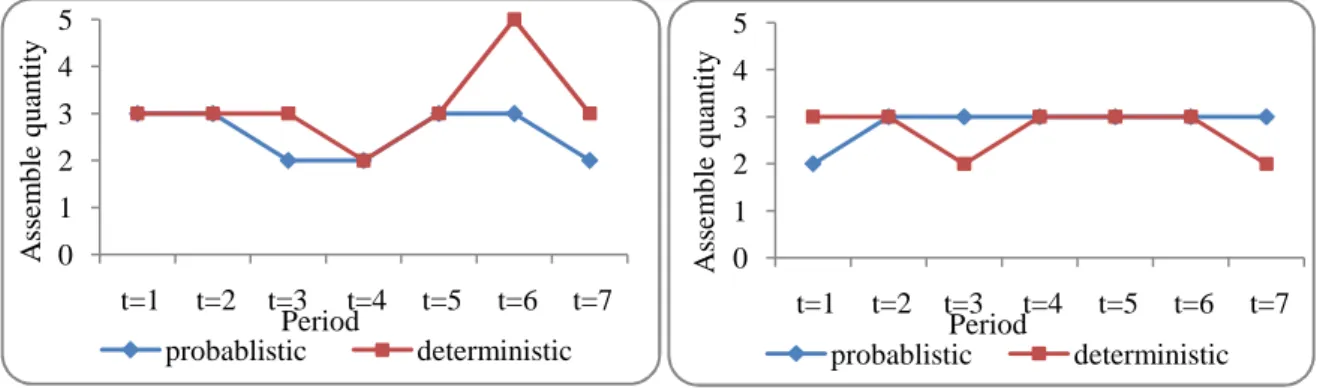
Figure 1 shows that the coefficient of variations for the assembly quantities in different periods on both lines in deterministic case is 28.6% and 18.0%, respectively. The corresponding values in probabilistic case are 18.0% and 13.2%, respectively. This means that the scheduling stability on both assembly lines is better in probabilistic case.
(a) Assembly line 1(b) Assembly line 2
Fig 1. Comparing the schedule of assembly lines in two cases.
Now, the effect of confidence level for the availability of sub assemblies (1-α) on the objective function is analyzed. As seen in table 8, by increasing the confidence level from 80% to 90%, the total costs go higher since more overtime is needed. However, as the confidence level becomes higher, the risk related to the lack of availability to the subassemblies is reduced.
Table 8. Objective function values in different confidence levels Confidence level
80% 85% 90%
First level O.F. 489.57 491.04 492.86
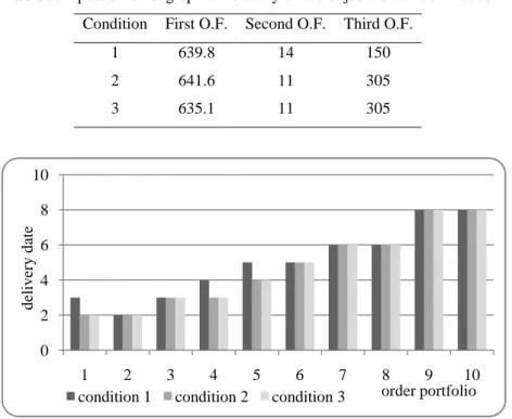
To examine the impact of lexicographic hierarchy on the objective function values, we consider the following three conditions: 1) current status, 2) second objective function is in level one while first and third ones are in level two, and 3) the objective functions are in different levels, respectively. In table 9, the objective function values are reported in each condition. Notably, first objective function (capacity-related costs) with nearly 1% reduction from 641.6 to 635.1 is not sensitive to the priority level. In contrast, the second and third ones are very sensitive to the hierarchy sincethey decrease as 27.2% and 50.8%, respectively. Figure 2 shows the impact of lexicographic hierarchy on the completion date of order portfolios.
0 1 2 3 4 5
t=1 t=2 t=3 t=4 t=5 t=6 t=7
A ss em b le q u an ti ty Period probablistic deterministic 0 1 2 3 4 5
t=1 t=2 t=3 t=4 t=5 t=6 t=7
A ss em b le q u an ti ty Period probablistic deterministic
Table 9.Impact of lexicographic hierarchy on the objective function values Third O.F.
Second O.F. First O.F.
Condition
150 14
639.8 1
305 11
641.6 2
305 11
635.1 3
Fig 2. Impact of lexicographic hierarchy on the tardiness/earliness of order portfolios
In order to address the effect of the proposed objective functions, we establish the following cases:
A: a single objective model of minimizing the capacity-related costs (First objective function)
B: a single objective model of minimizing the completion time dispersions of product models in order
portfolios (Second objective function)
C: a single objective model of minimizing the tardiness/earliness penalties (Third objective function) D: the proposed model in current status of lexicographic hierarchy.
The objective function values for the above four cases are given in table 10. The first and second objective function values increase in the multi-objective model compared to the single objective one. The value of second objective increase 27%, that’s because it conflicts with two other functions, that when these two functions impose as a constraint takes away from optimal value. But because of the importance of goals, decision maker prefers to consider model as multi objective. Table 11 gives the early/tardy order portfolios in different cases (as a measure of customer satisfaction).
Table 10. The objective function values for the single and multi-objective models Third O.F.
Second O.F.
First O.F.
Case
-635.1 A
-11
-B
150
-C
150 14
639.8 D
According to tables10 and 11, taking the multi-objective model into account is better because none of the order portfolios faced earliness. And also taking into account the multi objective model leads that don’t ignore any of the objectives of decision maker and the values of objective functions will improve.
0 2 4 6 8 10
1 2 3 4 5 6 7 8 9 10
d
el
iv
er
y
d
at
e
order portfolio
Table 11.Early/Tardy order portfolios in different cases D C B A Case -1,4,5 1,4,5 Early order portfolios
9 9 9 9 Tardy order portfolios
In the proposed model, we employ the concept of joint lot sizing. This means that for the economic considerations, a given lot size of an assembly line may be comprised of the order quantities of a given final product model in several order portfolios.
Tables12and 13, respectively, show the current assembly scheduling of company and the assembly scheduling of proposed model. Notably, the current assembly scheduling of company does not consider to the joint lot size and tries to assemble the same as the order size in any period (except for the first period which also compensates the initial shortage). For example, because of the lack of capacity in the first period, the initial shortage of AVR is not compensated; this trendalso continues in periods 2 and 3, and the shortage is transferred to period 4. This causes significant shortage costs in periods 1 to 3 and overtime cost in period 4. Also, one unit of MV product is not assembled in period 5 and moved to period 6; therefore, the order portfolio 8 is delivered one day late.Moreover, the current assembly scheduling employs the greater capacity in periods 1, 4 and 6 compared to the proposed model. The above considerations confirm that to make better use of the capacity, timely compensation of shortages, and to prevent any tardiness in the order deliveries, it is better to consider the joint lot size for the assembly of products.
Table 12. Current assembly scheduling of company
Table13. Assembly scheduling of proposed model
In bellow, we summarize the main findings and managerial insights which can be presented based on the proposed model and case study.
• It is better to be considered multiple objectives simultaneously for assembly schedule, because compared to the single objective model; none of the order portfolios face the earliness.
•Also multi objective model helps decision maker to not ignore any of the objectives.
Period Assembled products (units)
7 6 5 4 3 2 1 1 1 1 0 2 2 2 MCC
Product LV 2 1 1 3 1 0 2
0 5 2 1 1 2 3 MV 2 0 1 1 1 1 0 AVR Period Assembled products (units)
7 6 5 4 3 2 1 1 2 0 0 2 2 2 MCC
Product LV 1 1 1 4 1 0 2
0 4 4 1 1 2 2 MV 2 0 1 0 1 1 1 AVR
• Given the priority of the objective functions, if all the related costs place in the first priority level and delivery time in the second one, none of the order portfoliosfacethe earliness and a greater reduction in total costs is resulted.
•Considering the uncertainty in the access to components causes no delay in the orders’ completion dates.
•Studying joint lot size in the assembly of products leads to a more proper scheduling of assembly sequence, and on time compensate of the beginning shortage.
5- Conclusion
This paper presents a chance-constrained multi-objective model for ATO systems under the uncertainty in the subassembly availabilities. To solve the model, the lexicographic method was used. In order to validate the proposed method, the real data from an electrical company was employed. The results showed that establishing the three objectives simultaneously, helps the company achieving a proper and practical schedule with less costs.We considered order portfolio for each customer to better coordinate the orders with the assembly scheduling tasks and the order portfolio can be delivered with the lowest delay. Also, considering the earliness and tardiness penalties caused to have timely order deliveries whileinvolving the uncertainty in the sub assembly availabilities resulted in a more stable schedule. Finally, concerning joint assembly lot size was also effective because it better uses the capacity. Future extensions may be to formulate the failure of machinery in the proposed model.
Acknowledgement
The authors would thank the Editor-in-Chief and the anonymous referees for their valuable comments to greatly improve the quality of this presentation
References
Axsäter, S. (2005). Planning order releases for an assembly system with random operation times.OR
Spectrum, 27(2-3), 459-470.
Chang, H-J., Su, R-H., Yang, C-T., & Weng, M. W. (2012). An economic manufacturing quantity model for a two-stage assembly system with imperfect processes and variable production rate.Computers & Industrial Engineering, 63(1): 285-293.
Cheng, T. C. E., Gao, C., & Shen, h.(2011).Production planning and inventory allocation of a single-product assemble-to-order system with failure-prone machines. International Journal of Production Economics, 131(2): 604-617.
Chu, C., Proth, J-M., & Xie, X. (1993). Supply management in assembly systems. Naval Research Logistics,40(7):933-949.
Cniu, H. N., & Lin, T. M. (1988). An optimal lot-sizing model for multi-stage series/assembly systems.Computers & operations research, 15(5): 403-415.
DeCroix, G. A., Song, J-S.,& Zipkin, P. H. 2009. Managing an assemble-to-order system with returns.Manufacturing & service operations management, 11(1): 144-159.
Dolgui, A., & Ould-Louly, M-A. (2002). A model for supply planning under lead time uncertainty.International Journal of Production Economics, 78(2): 145-152.
Dolgui, A. B., Portmann, M. C., &Proth, J. M. (1996). A control model for assembly manufacturing systems.System Modelling and Optimization, 519-526.
DeCroix, G.A., & Zipkin, P. H.(2005). Inventory management for an assembly system with product or component returns.Management Science, 51(8): 1250-1265.
Elhafsi, M. (2009). Optimal integrated production and inventory control of an assemble-to-order system with multiple non-unitary demand classes. European Journal of Operational Research, 194(1): 127-142.
Elhafsi,M.,& Hamouda, E. (2015). Managing an assemble-to-order system with after sales market for components.European Journal of Operational Research, 242(3): 828-841.
Gurnani, H., Ram, A., & Lehoczky, J. (1996). Optimal order policies in assembly systems with random demand and random supplier delivery.IIE transactions,28(11): 865-878.
Hnaien, F., Delorme, X., & Dolgui, A. (2010). Multi-objective optimization for inventory control in two-level assembly systems under uncertainty of lead times.Computers & operations research, 37(11): 1835-1843.
Hnaien, F., Delorme, X., & Dolgui, A. (2009). Genetic algorithm for supply planning in two-level assembly systems with random lead times.Engineering Applications of Artificial Intelligence, 22(6): 906-915.
Horng, S-C., & Lin, S-S. (2017). Ordinal optimization based metaheuristic algorithm for optimal inventory policy of assemble-to-order systems.Applied Mathematical Modelling,42: 43-57.
Karaarslan, A. G., Kiesmüller, G. P., & De Kok, A. G. (2013). Analysis of an assemble-to-order system with different review periods.International Journal of Production Economics, 143(2): 335-341.
Kumar, A.(1989). Component inventory costs in an assembly problem with uncertain supplier lead-times.IIE transactions,21(2): 112-121.
Mokhtari, S., Madani, K., & Chang, N-B. (2012). Multi-criteria decision making under uncertainty: application to the California’s Sacramento-San Joaquin Delta problem.World Environmental and Water Resources Congress.
Olhager,J., and Wikner,J. (1998). A framework for integrated material and capacity based master scheduling.In Beyond Manufacturing Resource Planning (MRP II),3-20.
Proth, J. M., Mauroy, G., Wardi, Y., Chu, C., & Xie, X. L. (1997). Supply management for cost minimization in assembly systems with random component yield times.Journal of Intelligent Manufacturing, 8(5): 385-403.
Song, D. P., Hicks, C., & Earl, C. F. (2002). Product due date assignment for complex assemblies.International Journal of Production Economics, 76(3): 243-256.
Tang, O., & Grubbström, R. W.(2003). The detailed coordination problem in a two-level assembly system with stochastic lead times.International journal of production economics, 81-82(11): 415-429. Wang,X.J. (2014). On Assemble-to-order Systems", PhD Thesis, McMaster University.
Wemmerlöv,U. (1984). Assemble-to-order manufacturing: implications for materials
management.Journal of Operations Management,4(4): 347-368.
Xiao, Y., Chen, J., & Lee, C-Y. (2010). Optimal decisions for assemble-to-order systems with uncertain assembly capacity.International Journal of Production Economics, 123(1): 155-165.
Yano, C. A. (1987). Stochastic leadtimes in two-level assembly systems.IIE transactions, 19(4): 371-378.