Model synthesis

(1)

Model Synthesis

Paul C. Merrell

A dissertation submitted to the faculty of the University of North Carolina at Chapel Hill in partial fulfillment of the requirements for the degree of Doctor of Philosophy in the Department of Computer Science.

Chapel Hill 2009

Approved by:

Dinesh Manocha, Advisor

Jack Snoeyink, Reader

Benjamin Watson, Reader

Anselmo A. Lastra, Committee Member

(2)

(3)

Abstract

Paul C. Merrell: Model Synthesis. (Under the direction of Dinesh Manocha.)

Three-dimensional models are extensively used in nearly all types of computer graphics applications. The demand for 3D models is large and growing. However, despite extensive work in modeling for over four decades, model generation remains a labor-intensive and difficult process even with the best available tools.

We present a new procedural modeling technique called model synthesis that is designed to generate many classes of objects. Model synthesis is inspired by developments in texture synthesis. Model synthesis is designed to automatically generate a large model that resembles a small example model provided by the user. Every small part of the generated model is identical to a small part of the example model. By altering the example model, a wide variety of objects can be produced.

(4)

Acknowledgments

Writing this thesis has been a long, but satisfying journey full of facinating,

perplex-ing, and sometimes terribly frustrating problems. Through it all, I knew I could count

on the support of friends and colleagues to boost my spirits.

I’m indebted first and foremost to my advisor Dinesh Manocha. I’m grateful for his

steadfast support and for the many nights he helped me frantically finish papers before

the deadline. More than anything, I’m grateful for the confidence he placed in me. Early

on, there were so many reasons he could have doubted me and questioned the value of

my work, but he believed in me and offered me the freedom to explore a subject that

I’m most passionate about.

I’m thankful to Ming Lin, Ben Watson, Anselmo Lastra, and Jack Snoeyink for

serving on the committee. Thanks to Anselmo for his abundant kindness and words of

advice. Thanks to Ben for his procedural modeling expertise and for letting me renege

on a promise I made to become his student at NC State. Thanks to Jack for his deep

mathematical insights and for giving me lots of feedback.

Special thanks goes to Jess Martin who was the first person to show real enthusiasm

and encouragement for my work. Thanks to Peter Wonka, Jeremy Wendt, and Phillipos

Morodhai for reading some of my papers and suggesting revisions. Thanks to Vivek

Kwatra for interesting conversations about texture synthesis and for providing Figure

2.10(c). Thanks to my officemates David Gallup, Brian Clipp, and Christian Lauterbach

for being welcome distractions from the daily grind. Thanks to all the faculty, staff, and

students at UNC for making my time here pleasant and fulfilling.

I’m deeply grateful to Mom, Dad, Brian, Christine, Douglas, Shannon, and Amy

(5)

papers they read through them just to fix my grammatical and punctuational mistakes.

I’m especially grateful to Dad for always being willing to listen to my ideas even the

bizzare and incomprehensible ones. Thanks to Douglas for writing a powerful graphing

program that I used in Figure 3.8.

Thanks to many friends especially in the Durham Third Ward for making life in

Chapel Hill exciting and memorable.

This work was supported in part by W911NF-04-1-0088, NSF award 0636208, DARPA

/ RDECOM Contracts N61339-04-C-0043 and WR91CRB-08-C-0137, Intel, and

(6)

List of Tables

3.1 The model sizes, number of labels k, and computation times for each generated model. . . 65

(11)

List of Figures

1.1 Self-Similarity Occurs in Natural and Man-Made Objects . . . 2

1.2 Texture Synthesis Example . . . 3

1.3 Model Synthesis Input and Output . . . 4

1.4 Model Pieces, Consistent and Inconsistent Models . . . 6

1.5 Example illustrating the model synthesis algorithm. . . 7

1.6 Continuous Model Synthesis Overview . . . 9

1.7 Examples of the Variety of Shapes Model Synthesis can Produce . . . 10

2.1 Procedurally Generated Buildings by M¨uller et al. [40] . . . 13

2.2 Illustration of Efros and Leung’s Algorithm . . . 16

2.3 Illustration of Patch-Based Texture Synthesis . . . 17

2.4 Results from several methods that extend texture synthesis into modeling 20 2.5 Model Pieces . . . 21

2.6 Typical Shapes used in Modeling . . . 22

2.7 Typical Textures used in Texture Synthesis . . . 23

2.8 Texture Synthesis Failure Case . . . 24

2.9 Texture Synthesis Results on Triangle and Rectangle . . . 25

2.10 Texture Synthesis Results on a Cross-Shaped Input . . . 26

2.11 Failure of Patch-Based Texture Synthesis . . . 26

3.1 Examples of two-dimensional models . . . 30

(12)

3.4 Example illustrating the model synthesis algorithm. . . 38

3.5 Model Synthesis Failure Case . . . 43

3.6 Model Synthesis Delayed Failure Case . . . 44

3.7 An Example of a Planar 3-SAT Problem Reduced to a Model Synthesis Problem . . . 46

3.8 The success rate for various model sizes and different example models. . . 48

3.9 Example illustrating how parts of the model are modified. . . 50

3.10 Example demonstrating that some consistent models cannot be produced with a small block size. . . 53

3.11 Example illustrating the problems that may occur at the boundaries of the model . . . 54

3.12 Line Example Model, E . . . 58

3.13 Every possible consistent region with three or fewer labels. . . 59

3.14 No matter what is added to aR9 region, none of the neighboring catalogs become empty. . . 59

3.15 An Infallible Model Similar to a Fallible Model . . . 62

3.16 An Infallible Model Similar to another Fallible Model . . . 63

3.17 Parliament Building Result . . . 66

3.18 Castle Result . . . 67

3.19 Escheresque Result . . . 68

3.20 City Result . . . 69

3.21 Canyon Result . . . 70

3.22 Tree Result . . . 71

3.23 Given a few rotating gears (a), model synthesis generates complex ma-chinery (b). . . 72

3.24 Building Exterior and Interior Result . . . 73

(13)

3.26 Constrained Models . . . 77

3.27 A Time-Varying Model . . . 79

4.1 Discrete Model Synthesis Assumes that Models are Aligned to a Grid . . 81

4.2 Discrete Model Synthesis Assumes the Objects are Spaced according to the Grid . . . 82

4.3 Using a Smaller Grid may Improve the Results . . . 83

4.4 The Continuous Adjacency Constraint . . . 84

4.5 Problems with using Only Point-Sized Model Pieces . . . 86

4.6 A 1D Consistent Model . . . 89

4.7 A 2D Continuous Example Model . . . 91

4.8 Example Model of Two Discrete Objects . . . 96

4.9 ComputingCMt . . . 97

4.10 Overview of the Continuous Model Synthesis Algorithm . . . 104

4.11 Overview of the Algorithm with a Different Input Shape . . . 105

4.12 Vertex Figures of Various Points on a Triangle . . . 107

4.13 Vertex figure of a concave vertex. . . 107

4.14 Boolean expressions with two different object types . . . 108

4.15 Possible labels of a horizontal edge . . . 109

4.16 Possible labels of a vertex . . . 110

4.17 Various Neighborhoods Described using Boolean Expressions . . . 111

4.18 A Complex Vertex Described using a Boolean Expression . . . 112

4.19 Parallel Planes Created in the 3D Case . . . 113

4.20 The possible labels of a 3D vertex found in the input model. . . 114

(14)

4.22 The evolution of the list of possible labels CMt over time. . . 119

4.23 A model can be created by modifying only part of it at once . . . 120

4.24 Examples of neighborhoods that involve more than four half-spaces . . . 121

4.25 Dimensional Constraint . . . 125

4.26 Large-Scale Constraints . . . 127

4.27 Bounding Volumes used to Simplify a Complex Shape . . . 128

4.28 Skyscaper Results . . . 130

4.29 Fractal Results . . . 131

4.30 Landscape Results . . . 132

4.31 Arches Results . . . 133

4.32 House Results . . . 134

4.33 From the input model (a), stairs are automatically generated (b). . . 135

4.34 Pentagon-Shaped Building Results . . . 136

4.35 Oil Platform Results . . . 137

4.36 Result with Non-Trihedral Vertices . . . 138

4.37 Spaceship Results . . . 139

4.38 Road Network Results . . . 140

4.39 Plumbing Results . . . 141

4.40 Roller Coaster Result . . . 142

5.1 Comparison of Texture Synthesis and Model Synthesis Results . . . 146

5.2 Comparison of Texture Synthesis and Model Synthesis Results . . . 146

5.3 Examples of Grammars used in Modeling . . . 150

5.4 Converting a 3D Model into a 1D string . . . 151

(15)

5.6 An Example of a Closed Path . . . 158

5.7 An Example of a Closed Path Generated by a Grammar. . . 160

(16)

List of Symbols

E Input Example Model

M Generated Output Model

nx×ny ×nz The length, width, and height of M

n0_x×n0_y ×n0_z The length, width, and height of E K The set of Possible Labels

k The number of elements in K

ˆı,ˆ,kˆ Unit vectors in the x,y, and z directions

Tx, Ty, Tz The Transition Matrices

DE(nx, ny, nz) The number of solutions for a given size

C?

Mt The ideal catalog of possible labels

CMt The imperfect catalog of possible labels

∃ There exists

∀ For all

⇒ implies that

u List of positions to update

(17)

mx×my×mz The size of the block to modify

Ri The i-th possible region inM

⊕ Minkowski Sum

Vi The extent of object i

vf The vertex figure

m The number of distinct normals

n The number of planes for each normal

h1, h2, . . . hm The set of half-spaces or half-planes

s1, s2, . . . sm The plane spacings

n1,n2, . . .nm The face normals

hC

i The complement of hi

(18)

Chapter 1 Introduction

Three-dimensional geometric models are used to represent the shape and design of

objects in nearly every type of computer graphics application including virtual

envi-ronments, CAD/CAM, computer gaming, animated movies, and medical simulations.

These applications require complex 3D models to be realistic and compelling. The

de-mand for detailed 3D models is large and expanding. However, satisfying the dede-mand

for models is difficult. Realistic models often contain very complex and widely varying

shapes and styles. Modeling can be tremendously time-consuming. For example, the

urban models created for the movie Superman Returns took 15 man years to complete

[40].

Modeling is a creative and artistic process. The objects being modeled may not be

based upon real objects, but purely on an artist’s imagination. Modeling involves many

artistic and high-level design decisions. Decisions about the style and purpose of each

object must be made to produce compelling models. Even though creative decisions are

an integral part of modeling, in practice, users spend more effort on routine and tedious

tasks.

Despite extensive work in geometric modeling for over four decades, it remains a

labor-intensive and difficult process even with the best available tools. Current modeling

(19)

and even when the tools are mastered creating complex models is still difficult. With

state of the art 3D CAD and modeling tools such as Autodesk’s 3D Studio Max and

Maya, the user can create simple geometric primitives and modify them using various

transformations and geometric operations. Modeling complex environments such as

cities or a landscapes requires creating and manipulating a huge number of primitives

and can take many hours or days [40].

Fortunately, there are many reasons to believe that the modeling process can be

greatly simplified and automated. Modeling involves many routine and repetitive tasks.

Many of the objects in games, movies, and virtual environments contain repetitive and

self-similar structures. Self-similarity is common in man-made objects and natural

ob-jects [38] (Figure 1.1). Self-similarity is often used to simplify and automate the

mod-eling process. Automation is the goal of procedural modeling techniques. In procedural

modeling, automatic procedures are used to generate models.

(a) Photograph of a Fern (b) Photograph of Prague

Figure 1.1: Objects with repetitive or self-similar structures tend to be procedurally modeled more easily. Self-similarity is a common feature of both man-made and natural objects.

This thesis explores a new procedural modeling technique that is designed to apply

broadly to many classes of objects. It is inspired by recent developments in the texture

synthesis literature [15, 74]. Textures are loosely defined as images containing some

(20)

that resembles an example texture. For example, from the small example in Figure

1.2(a) a texture synthesis algorithm would generate the large texture in Figure 1.2(b).

Texture synthesis is based upon the user specifying what the algorithm should generate

by providing an example. Texture synthesis is one of many techniques which use this

example-based principle. Example-based techniques are also used for generating high

resolution images from low resolution images [18], for filtering images so they resemble a

particular painting or drawing [24], for skinning [56], and for generating curves [25]. By

using an example, the user can often specify what kind of results should be produced

more easily and more intuitively. Example-based techniques often apply more generally

to a wider variety of models than other methods [74]. For example, texture synthesis

methods which use examples can generate a wider variety of textures than other methods

such as Perlin noise [47]. Even though example-based techniques have been applied to

many areas of graphics, their use in modeling has been limited [19].

(a) Exam-ple Input Texture

(b) Output Texture

Figure 1.2: Texture synthesis algorithms take a small input example texture (a) and produce a new texture (b) that resembles it.

In an example-based modeling technique, the user would provide a small example

model (Figure 1.3(a)) and then the algorithm would generate a larger model that

(21)

because it is similar to texture synthesis. Designing this type of algorithm for 3D models

is the central goal of this thesis.

(a) Example Input Model (b) Synthesized Output Model

Figure 1.3: Model Synthesis Input and Output

1.1 Thesis Statement

We introduce an procedural modeling algorithm that allows a 3D modeler to generate

a variety of complex and rich environments relatively quickly and easily by using

exam-ple. Our model synthesis algorithm can efficiently generate large models containing flat

polyhedral shapes common in architecture.

1.2 Thesis Goals

The thesis has four main goals:

(22)

• To analyze the strengths and limitations of such algorithms including their time and memory requirements.

• To demonstrate of the generality of these algorithms by modeling many diverse complex objects and environments.

• To impose several additional user-defined constraints on the generated model.

This thesis focuses on one central problem of generating a new 3D model that

resem-bles a given input model. Models may resemble one another for a variety of reasons, so

the notion of resemblance needs to be defined more precisely. A similar issue is

encoun-tered in the texture synthesis literature: many texture synthesis algorithms are based

on the principle that two textures resemble one another if the patches of texture they

contain are similar. More precisely, two textures resemble one another if every small

patch in one texture is similar or identical to a small patch in the other. The same

principle could be applied to 3D models. Models resemble one another if every small

part of one model is identical to some part of the other.

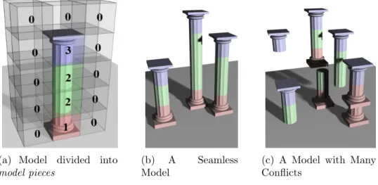
We consider two different model synthesis approaches: discrete model synthesis and

continuous model synthesis. In discrete model synthesis, the user divides an input

model into discrete building blocks called model pieces shown in Figure 1.4(a). The

model pieces are also called labels, since every point in a 3D array is labeled according

to which model piece occupies it. Discrete model synthesis is simpler than continuous

model synthesis and is discussed first.

The goal of model synthesis is to generate a new model in which each pair of adjacent

labels exactly matches a pair of adjacent labels in the input model. This is called the

adjacency constraint. The effect of the constraint is illustrated in Figure 1.4. Figure

1.4(b) satisfies the constraint, but Figure 1.4(c) violates it. The adjacency constraint

(23)

(a) Model divided into

model pieces

(b) A Seamless Model

(c) A Model with Many Conflicts

Figure 1.4: In discrete model synthesis, the user divides the model into model pieces (a). The goal is to generate a new model whose pieces fit seamlessly (b). If the pieces do not fit together, the model (c) does not resemble the input.

resembles the input. By always satisfying this constraint, model synthesis improves

upon texture synthesis. Current texture synthesis algorithms do not always satisfy

the constraint. They may generate textures containing parts that do not fit together

properly and conflict with each other. These conflicts occur because existing texture

synthesis algorithms check only the local neighborhood around a pixel when it is added.

The model synthesis algorithm searches for possible conflicts globally, so it can find and

avoid conflicts between the labels more effectively. This global search is particularly

valuable for model synthesis, but it is also useful for texture synthesis. The search is

performed using a catalog of possible labels that could be added. An example of this

catalog is shown in Figure 1.5. Each label corresponds to a model piece. Labels are

removed from the catalog, if they conflicts with the current model. Each removal may

cause other adjacent labels to be removed. The removals may propagate through the

array. So a possible conflict in one of the locations may cause labels to be removed in

a distant location. When labels are added into the model, they are selected from the

(24)

(a) Example Model,E (b) Incomplete ModelM (c) Catalog of labels to add, CM

Figure 1.5: For the example model E (a) and the incomplete modelM(b), a catalog of possible assignments is computed (c).

However, this global search may not be able to detect every conflict. In fact, detecting

all conflicts when generating a large model can be extremely difficult. To show this, we

present an NP-completeness proof in Theorem 3.3.5. An undetected conflict can cause

the catalog to become empty. This is a serious problem since then there would no

labels to choose from and the adjacency constraint would be violated. If the catalog

becomes empty, the algorithm in its initial form fails. To handle failures, we introduce a

second algorithm. The second algorithm is based upon the observation that the initial

algorithm succeeds much more frequently when generating small models. The second

algorithm creates large models in small parts. If a failure occurs when creating one of

the small parts, the algorithm backtracks slightly and continues.

In summary, model synthesis improves upon texture synthesis in two key ways. First,

it uses a global search to find and avoid conflicts and second, it creates the model in

parts. With these improvements, it can generate models where all of the model pieces

fit together seamlessly.

The discrete and the continuous model synthesis problems are both solved by using a

global search and by modifying in parts. The key difference between them is that discrete

model synthesis represents the models as an array of labels as shown in Figures 1.4(b)

(25)

that has been decomposed into discrete model pieces that fit on a grid. The algorithm

works well if it is given a good example model. But providing the example model can

be difficult since many models do not fit naturally onto a grid. If the model does not fit

well on a grid, then model synthesis cannot generate interesting new variations similar

to the input. The algorithm generates only exact copies of the input. This problem is

caused by using discrete model pieces. An algorithm that does not use discrete model

pieces could overcome this problem. Rather than trying to assign labels to every discrete

point on a grid, a better goal would be to assign labels to every point in 3D space i.e.

continuous model synthesis. The goal is still to assign labels that satisfy an adjacency

constraint, but the points are now in the continuous domain. Discrete and continuous

model synthesis share many of the same concepts. Both methods use a catalog of possible

labels, but the catalog is much more difficult to compute in the continuous case. The

continuous domain includes an infinite number of points, so the catalog may contain an

infinite number of possible assignments and the catalog is recorded geometrically rather

than in an array. We propose several different ways of computing this catalog, but some

of them are too difficult to implement. One way to greatly simplify the continuous

problem is to assume that the faces of the output lie on a set of planes parallel to the

input. This assumption imposes an additional constraint on the output which can limit

the range of possible results in some cases.

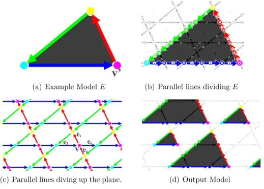
An overview of the continuous model synthesis algorithm is shown in Figure 4.10.

Starting with the input example shape shown in Figure 1.6(a), we create sets of lines

parallel to the edges of the input as shown in Figure 1.6(c). These lines divide the

plane into an arrangement of faces, edges, and vertices. Each face, edge, and vertex is

associated with a set of acceptable neighborhoods or labels that satisfy the adjacency

constraint. The set of possible labels could be computed by dividing the input model

along parallel lines as shown in Figure 1.6(b). The remaining steps of the algorithm

(26)

to search globally for potential conflicts and the model can be modified in parts. The

algorithm generates an output model satisfying the adjacency constraint such as Figure

1.6(d).

(a) Example ModelE (b) Parallel lines dividing E

(c) Parallel lines diving up the plane. (d) Output Model

Figure 1.6: Continuous Model Synthesis Overview. Lines parallel to the input shape (a), divide the plane into faces, edges, and vertices (c). The output shape (d) is formed within the parallel lines. The set of acceptable vertex and edges labels in the output (d) can be found by dividing the input along parallel lines (b).

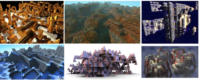
Overall, model synthesis offers many benefits. Most other procedural modeling

tech-niques are targeted to a specific type of object, but model synthesis can generate a wide

variety of objects and environments including cities, landscapes, plants, fractal

struc-tures, castles, cathedrals, spaceships, roller coasters, oil platforms, building interiors and

more. A few examples are shown in Figure 1.7. In each case, the only user input is a

simple example model.

The primary goal of both discrete and continuous model synthesis is to satisfy the

adjacency constraint, but many additional user-defined constraints should be used to

create more realistic models. The user might have a floor plan or a general idea of what

(27)

Figure 1.7: Examples of the wide variety of shapes that our model synthesis algorithm can generate including machinery, landscapes, spaceships, castles, fractals, and oil plat-forms.

that are symmetric. These constraints and many others can be imposed on the models

with our framework.

1.3 Chapter Overview

The rest of the thesis is organized as follows. Chapter 2 surveys related work in

proce-dural modeling and texture synthesis. Section 2.3 discusses differences between textures

and 3D models that explain why texture synthesis techniques generate 3D models less

effectively.

Chapter 3 discusses discrete model synthesis. The problem is formally described in

Section 3.1. It is shown that the number of possible solutions may grow exponentially

with the output size. An algorithm for finding solutions is described in Section 3.3 and its

time complexity is analyzed. Unfortunately, this algorithm fails to complete properly

in some cases. The catalog may become empty and the algorithm cannot continue.

Section 3.3.5 shows with an NP-completeness proof that in some cases these failures are

(28)

if they occur.

Chapter 4 discusses continuous model synthesis. Section 4.1 explains why

continu-ous model synthesis is needed by discussing the limitations of discrete model synthesis.

Several different approaches are introduced. Sections 4.3 and 4.4 describe two different

approaches that could be used, but these approaches have several serious

implementa-tion issues. For example, one approach has not been implemented because it requires

exact and robust 3D Boolean operations and 3D Minkowski sum computations. Section

4.5 describes a more practical approach that is much simpler to implement because it

assumes that the models are generated on sets of parallel planes. This parallel plane

as-sumption introduces some limitations which are also discussed. Also, other constraints

beyond the adjacency constraint are described for controlling the output more effectively.

Model synthesis is compared with texture synthesis in Section 5.1 and with other

procedural modeling techniques in Section 5.2. Model synthesis is also compared with

formal grammar and a close relationship between them is established.

Chapter 6 summarizes the main points of the thesis and discusses exciting

(29)

Chapter 2 Related Work and Background

This chapter discusses work related to model synthesis in the fields of procedural

mod-eling and texture synthesis. Section 2.3 discusses differences between texture synthesis

and model synthesis and how texture synthesis might be extended to 3D modeling and

why a new algorithm is needed for model synthesis.

2.1 Procedural Modeling

Many procedural modeling techniques have been developed over the last few decades.

These techniques as a group have a great amount of variety in the approach they take.

Most techniques are targeted at modeling a specific type of object or environment. Early

techniques based on fractal geometry achieved some success modeling natural landscapes

[17]. A connection between landscapes and fractal geometry was observed in the 70s

[38]. Mandelbrot observed that a record of Brownian motion over time resembles an

outline of jagged mountain peaks. Models of landscapes can be further improved by

considering how landscapes erode over time [42].

There also is a long history of modeling plants procedurally. Many plant modeling

techniques use a formal grammar call an L-system. L-systems were proposed by

Lin-denmayer as a general framework for describing plant growth and plant models [35, 52].

(30)

how plants interact with their environment as they grow [39]. Many techniques also

use information supplied by the user to influence the shape of the plant models such as

positional information [53], sketches of plants [6], or photographs [54, 61].

Many techniques are designed targeted specifically for modeling urban models

proce-durally [69, 65]. Like many plant modeling techniques, some urban modeling techniques

use L-systems. L-systems have been used to generate road networks from elevation and

population density data and to generate buildings on parcels of land between the roads

[44]. Other grammars have been introduced specifically for modeling architecture. The

architect, Stiny [1971] introduced shape grammars as a tool for analyzing and designing

architecture. Shape grammars remained largely a conceptual tool [59, 16] until Wonka

and others introduced a related group of grammars called split grammars [75]. Split

grammars operate by splitting shapes into smaller components and can generate highly

detailed models of architecture. Split grammars were further developed by M¨uller et al.

[40] who include shape operations for mass modeling and for aligning many parts of a

building’s design together. Their method can generate both the large-scale layout of a

city as well as many geometric details within each building to produce a highly complex

and realistic city. Tools have also been developed to edit these grammars visually using

a GUI [36] and for deriving grammars automatically from images of facades [41]. A

method developed by Aliaga et al. [1] constructs grammars from photographs with the

user guiding the creation and subdivision of an initial 3D model.

(31)

Another group of techniques focuses more heavily on the 2D layouts of cities than

on the 3D shapes of the buildings. Chen et al. [5] allow users to edit a city’s street

layout interactively using tensor fields. Aliaga et al. [2] generate street layouts using an

example-based method. This is particularly relevant as their method combines elements

of texture synthesis and procedural modeling. The streets are generated like other

pro-cedural modeling techniques and then an image of the city seen from above is generated

like a texture using texture synthesis. A related area of research is urban simulation.

Much of the research into urban simulation is conducted outside of computer graphics

where the purpose is not to model and render cities, but to understand how various

factors influence a cities development and growth over time [63, 67]. However, this area

of research is certainly relevant to computer graphics and several authors have

incorpo-rated aspects of urban simulation into their methods to produce more realistic models

of cities [70, 33]. Their methods simulate part of a city’s economy and generate street

layouts and zone the land area for different economic activities.

There are also other techniques designed to model much smaller structures than

cities. Legakis et al. [34] propose a method for automatically embellishing 3D surfaces

with various cellular textures including bricks, stones and tiles. Cutler et al. [11]

de-veloped a method for modeling layered, solid models with an internal structure. Their

method can modify models by simulating various physical processes such as erosion and

fractures. Another method has been developed to model truss structures by optimizing

the locations and strengths of beams and joints that support bridges, tower platforms,

and other objects [58]. Pottmann et al. [49, 50] have developed algorithms based on

discrete differential geometry that determine how to arrange beams and glass panels so

they form in the shape of a given freeform surface and satisfy various geometric and

physical constraints.

Another way to model objects is to combine together parts of existing models

(32)

to find a desired part, then cut the part out from the model, and stitch various parts

together to create a new object.

2.2 Texture Synthesis

Although model synthesis is designed for procedural modeling, the algorithm itself has

more in common with texture synthesis. The field of texture synthesis has seen many

exciting new developments over the past decade. This section surveys these

develop-ments and explain their relationship to model synthesis. A more detailed survey is given

in [74].

2.2.1 Markov Random Fields

Textures are often described as Markov Random Fields [15, Zhu et al., 48, 43, 74].

Markov Random Fields have a set of random variables Xi. In this case, each random

variable represents the color of a pixel. Each pixel i has a set of neighbors surrounding it called Ni. It is often assumed that only the neighbors of pixel i determines its value.

This assumption is called the Markov locality property. Stated more formally, the color

of pixel i is conditionally independent of the pixel colors outside Ni, given the pixel

colors insideNi. This means the probability of Xi having the color xi has the following

property ∀x1, x2, . . .

P[Xi =xi | ∀j 6=i, Xj =xj] =P[Xi =xi | ∀j ∈Ni, j 6=i, Xj =xj] (2.1)

(33)

2.2.2 Texture Synthesis Algorithms

Over the past decade, the field of texture synthesis has seen a proliferation of new

algorithms and new ideas. Many of these algorithms were influenced by a seminal paper

written by Efros and Leung [1999]. Their algorithm is remarkably simple and produces

good results. Their algorithm generates textures by adding pixels individually. To

determine which pixel should be added at a given point, a small neighborhood around

the point is compared against every neighborhood in the example texture. The purpose

of the comparisons is to find which neighborhood matches the neighborhood around

the insertion point the closest. The quality of each match is evaluated using a sum of

squared differences. Figure 2.2 shows a set of close matches for a given neighborhood.

A neighborhood is a close match if it matches to within a certain percentage of the

closest match. From among every close neighborhood, one is randomly selected and its

central pixel is added into the new texture. Every pixel of the texture is added this way.

Efros and Leung’s method [1999] is one of the simplest texture synthesis algorithms. It

generally produces good results, but it does have some failure cases. The algorithm is

slow because computing an exhaustive nearest neighborhood search is expensive.

(a) Input Example Texture (b) Synthesizing a Pixel

Figure 2.2: Illustration of Efros and Leung’s Algorithm [1999]. To determine which pixel to insert at a given point, the neighborhood around the point is compared against other neighborhoods in the example texture. The pixel to insert is randomly selected from among the closely matching neighborhoods.

(34)

the center and adding pixels going out in concentric rings. However, by adding pixels in

a different order, the speed of the algorithm can be improved as shown by Wei and Levoy

[2000]. They developed a similar algorithm that adds the pixels in scan line order. Using

this order, the method can be accelerated using tree-structured vector quantization.

There are several other ways to accelerate texture synthesis. Several acceleration

techniques are based on the observation that groups of neighboring pixels in the input

are likely to be grouped together in the output. This is known as coherence.

Coher-ence is used in several methods to improve the performance [62, 3]. CoherCoher-ence can be

used to compute approximate nearest-neighborhood matches very quickly to be used in

interactive editing tools [3]. Another acceleration strategy is instead of adding pixels

individually, they can be added in large groups or patches. Patches of texture rarely fit

together seamlessly, but an optimal cut can be made between the patches so they fit

together without any noticeable seams as shown in Figure 2.3. The cuts can be made

either by using dynamic programming [14] or by using graph cuts [29]. Another

ap-proach to texture synthesis is to optimize a global energy function using an expectation

maximization algorithm [30].

(a) Patches Overlap (b) Patches are Stitched Together

Figure 2.3: In patch-based texture synthesis, different patches are copied and overlapped slightly. An optimal cut is computed between the two patches.

Textures are primarily used for texture mapping 3D models. Ordinarily, textures

are synthesized onto a flat texture map which is then applied to a curved surface, but

(35)

onto the curved surfaces. This can be accomplished with an orientation field covering

the surface [64, 72]. The orientation field specifies the direction of the texture and plays

the same role as the rows and columns of an array of pixels.

Several methods have extended texture synthesis into three dimensions. Some

meth-ods use a third temporal dimension to textures so that they move and change over time

[71, 29]. This is especially useful for creating moving images of fire, smoke, and running

water. These dynamic textures could also be described using linear dynamical systems

[12].

Another reason to extend texture synthesis into three dimensions is to create solid

textures [45, 46]. Solid textures are an alternative to 2D texture maps. They describe

many natural materials such as wood and stone more accurately than 2D texture maps

and they avoid the task of parameterizing the object’s surface which can be difficult.

Until recently, solid textures were created only with user specified procedure, but now

texture synthesis can be used [23, 28]. Solid texture synthesis starts like ordinary texture

synthesis from an input of a 2D texture, but the goal is to produce a 3D solid texture

which certain properties. It should be possible to slice the solid texture open to reveal

a pattern on the slice that resembles the input texture. Such a solid texture could be

generated by optimizing a global energy function [28] like some 2D texture synthesis

algorithms [30].

Texture synthesis has also been used to generate what are called geometric textures

[4, Zhou et al.] which are a combination of texture mapping and modeling. They are

used like texture maps to apply patterns to objects, but these patterns actually change

the shape of the object itself. This is useful for creating objects with bumps or dimples

(Figure 2.4(a)) or objects that are made out of chain mail (Figure 2.4(b)). Texture

synthesis has also been used to generate hair in different styles [68] and to create 3D

models of terrain using real elevation data as the example [76]. Texture synthesis has also

(36)

of objects [26].

Lagae, Dumont, and Dutr´e [2005] developed a method called geometry synthesis

which resembles model synthesis in some ways. Their method also extends texture

syn-thesis into three dimensions for procedural modeling. Their algorithm takes an input

model and computes a 3D array of signed distance values. This array is used as the

example and a new array is generated using a standard texture synthesis technique.

However, texture synthesis methods have difficulty with many inputs common to

mod-eling including very basic shapes as discussed in Section 2.3. The geometry synthesis

method is applied to models that have regular patterns as shown in Figures 2.4(c) and

2.4(d).

Some texture synthesis techniques use tiles to accelerate the algorithm. Tiles are

particularly relevant to model synthesis since model pieces are essentially 3D tiles. Most

of these methods use Wang tiles. Wang tiles were studied initially by mathematicians

interested in aperiodic tiling [10], but they have also been applied to texture mapping

and texture synthesis [Stam, 8, 31]. The 3D counterpart of a Wang tile is a Wang

cube. Wang cubes have been used to model asteroid fields [57] and render volume data

[37]. However, we show that it is often difficult to apply Wang tiles and Wang cubes to

modeling later in Section 5.1.1.

A few other advancements in texture synthesis should be mentioned. A multiscale

algorithm has been used to generate extremely high resolution textures [21]. The texture

synthesis process can be inverted to find a small representative example texture from a

large texture [73]. Texture synthesis can also be used to complete a missing part of an

image [9, 13, 60, 22]. This is especially useful for removing objects from images without

leaving holes. A few of the image-completion techniques change choosing the order in

which the pixels are added to improve the results [9, 60].

A related technique called context-based surface completion [55] completes models

(37)

(a) Geometric Textures (b) Mesh Quilting

(c) Chain Mail (d) Grid

Figure 2.4: Result from Geometric Textures (a) [4], Mesh Quilting (b) [Zhou et al.] and Geometry Synthesis (c & d) [32]. Each method extends texture synthesis in some way to generate models. The models have patterns that resemble textures. Geometry synthesis generates models from examples. The examples are shown in the insets (c & d).

in any missing regions with surfaces that resemble the rest of the model. In this case,

the rest of the model effectively acts as the example.

2.3 Differences between Textures and Models

Texture synthesis and model synthesis have similar goals. However, textures and models

differ in several important ways that affect how they are generated. An obvious difference

is that textures have two spatial dimensions while models have three, but most texture

(38)

texture synthesis algorithms have frequently been used to create three-dimensional solid

textures [28] or textures with a temporal dimension [71, 12, 29].

Textures are typically represented as arrays of pixels which store red, green, and blue

color values. Models are typically represented using geometric shapes such as polygonal

meshes or NURBS. Texture synthesis methods could be directly used for modeling if

the models were represented in an array. The elements of the array would be small

building blocks calledmodel pieces. Each model piece would contain textured geometric

shapes within a cubic volume of space as shown in Figure 2.5. Model pieces are similar

to texture patches or to tiles that some texture synthesis methods use [7]. The model

pieces are created by the user. The user could break an existing model down into model

pieces or could start by creating the model pieces and then build the model up with

them. Most model pieces should be in the model multiple times. Otherwise, the model

is not self-similar and the algorithm may not create interesting new variations off the

original model. However, it can sometimes be difficult to create the model so that the

model pieces repeat. These difficulties are described in Section 4.1. To overcome them,

we introduce continuous model synthesis which does not use model pieces in Chapter 4.

Figure 2.5: Model constructed out of model pieces.

Each model piece corresponds to a label. Labels are assigned to every point in a 3D

(39)

Model synthesis differs from texture synthesis because model pieces differ from pixel

colors in several ways. First, colors can easily be blended together. Mixing red and

yellow, produces orange. But model pieces are not so easily blended. The top of a

pyramid cannot easily be blended with the bottom of a sphere. Averaging the labels

1 and 3 does not produce the label 2. Another difference is that colors can easily be

positioned in a color space where similar colors are grouped together in the space. But

model pieces are different. The label 1 is not necessarily closer to label 2 than to label 15.

Model synthesis is in some sense stricter than texture synthesis. In texture synthesis, if

a color is close to the right value that often is good enough, but in model synthesis, that

is not good enough. For example, suppose some model pieces contain flat squares. The

model pieces fit together perfectly, if both squares are at exactly the same height, but

if one square is slightly higher then there is a noticeable hole in between them. Minor

changes to the model pieces can produce large errors.

There are other important differences between textures and models that go beyond

differences in the number of dimensions they use or between pixels and model pieces.

We demonstrate these other differences by running texture synthesis algorithms on 2D

shapes commonly found in models. Let us consider as an input two of the simplest

shapes: a triangle and a rectangle (Figure 2.6).

Figure 2.6: Typical Shapes used in Modeling

These shapes are common in geometric models. They could represent the floor plan of

(40)

can be used as an input into a texture synthesis algorithm, but surprisingly, texture

synthesis algorithms have difficulty even with these simple shapes. Although the shapes

in Figure 2.6 are typically used in modeling, they differ from typical textures used in

texture mapping or texture synthesis. A few representative examples of textures used in

texture synthesis are shown in Figure 2.7 for comparison. Each texture was generated

using a texture synthesis method by Kwatra et al. [2005].

(a) (b) (c) (d)

Figure 2.7: A few representative textures typically used in texture synthesis.

One difference between a typical textures and a typical shape used in modeling is

they have different types of boundaries. 3D models typically represent objects with a

few sharp well-defined boundaries between their interior and exterior. (One possible

exception might be a puff of smoke.) On the other hand, a texture has soft or hard

boundaries where its image intensity changes. The change could be soft and gradual or

a hard edge. Textures typically have many edges rather than a few prominent ones. For

example, Figure 2.6 only has seven edges, while Figure 2.7(d) has many more.

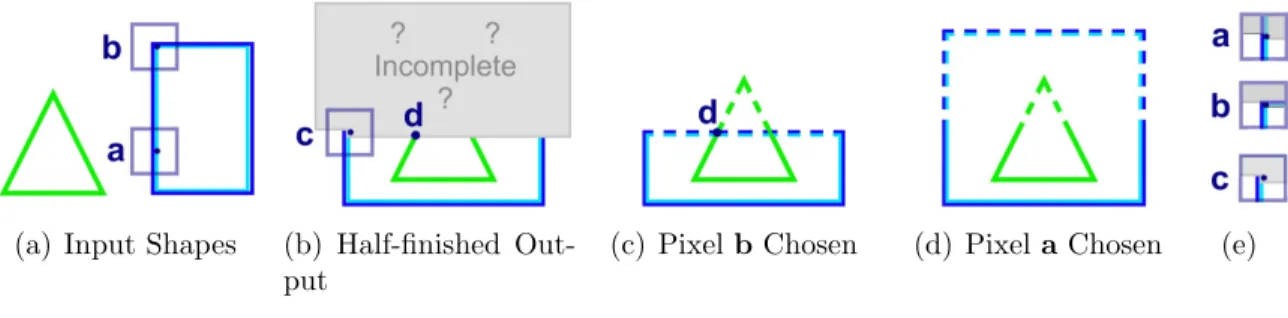
In order to better understand why texture synthesis algorithms have trouble with the

shapes in Figure 2.6, let us examine the synthesis process of a typical texture synthesis

algorithm. Let us examine Efros and Leung’s method [1999]. Suppose that about

halfway through the algorithm, it has produced a half-finished result as shown in Figure

2.8(b). The bottom half is finished, but the upper half has not been determined. The

(41)

by finding pixels with neighborhoods similar to pixels in the input in Figure 2.8(a). Let

us examine two of the alternatives: pixel aor pixel b.

(a) Input Shapes (b) Half-finished Out-put

(c) PixelbChosen (d) Pixela Chosen (e)

Figure 2.8: Some texture synthesis methods have difficulty with input (a). After half of the texture has been created (b), a decision is being considered at pixel c. If pixel

b from the input is used, the texture can not be completely properly (c). If pixel a is used, it can be completed (d). The bottom halves of the neighborhoods around pixels

a, b, and care the same (e).

Each alternative looks equally suitable if we examine only the neighborhood

sur-rounding pixel c. In fact, the neighborhoods around pixels a, b, and c have identical bottom halves (Figure 2.8(e)). Since Figure 2.8(b) is unfinished, we have no information

about what is above or directly to the right of pixel c. Locally, both choices appear to be equally good, but in practice, they are not. If pixel b is chosen, the algorithm will eventually fail. Once pixel b is chosen, the texture cannot be completed by using neighborhoods from the input (Figure 2.8(a)). There is only one way to complete the

rectangle which is shown in Figure 2.8(c), but the rectangle is bound to intersect the

triangle’s edge at pixeld. Edges should not intersect, because the input in Figure 2.8(a) does not contain any intersecting edges. If pixel a is chosen, the texture can be com-pleted successfully as shown in Figure 2.8(d). But there is no way of knowing that ais a better choice than b by only looking at local neighborhoods.

The choice of inserting the value atb into pixelcis unacceptable because of the tri-angle’s edge at pixeld. The value at pixeld influences the value at pixelc, even though these pixels are far from one another. In fact, even if Figure 2.8(b) were scaled up a

(42)

distance. This example demonstrates a problem common to many texture synthesis

al-gorithms which only examine local neighborhoods when making their decisions. At first

glance, the fact that pixeld influences pixelc while it is outside the local neighborhood of cmight appear to violate the locality assumption in Equation 2.1. But Equation 2.1 assumes the entire neighborhood Nc surround pixel c is known, but in Figure 2.8(b),

the values of the pixels directly above pixelc are unknown. So the locality assumption is not violated.

Figure 2.8 illustrates a single error that a texture synthesis algorithm could make,

but there are many more chances to make errors when synthesizing a large texture or

model as shown in Figure 2.9. Results from a different input shape are shown in Figure

2.10 in which numerous shapes fail to close.

(a) Input Shape

(b) Efros and Leung, 1999

Figure 2.9: Texture synthesis methods have difficulty with the triangle and rectangle input (a). Results from a texture synthesis method is shown (b).

Other texture synthesis techniques operate on patches of texture instead of

indi-vidual pixels. Similar problems occur when using patch-based methods. Patch-based

methods copy patches of texture together with some overlap and then cut and stitch the

overlapping parts together. An optimal cut is computed using dynamic programming

(43)

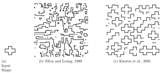
(a) Input Shape

(b) Efros and Leung, 1999 (c) Kwatra et al., 2005

Figure 2.10: Texture synthesis methods have difficulty with a cross-shaped input (a). Results from two different texture synthesis methods are shown (b,c).

2.3, but work poorly for an input like Figure 2.6. Two patches are copied from Figure

2.6 and placed into Figure 2.11 which shows the two patches cannot be stitched together.

Most patches copied from Figure 2.6 would have the same problem.

(a) Patches are Stitched Together

(b) Overlapping Patches

Figure 2.11: In patch-based texture synthesis, different patches are copied and over-lapped slightly. A optimal cut is supposed to be made, but none of the cuts are good.

Patch-based methods work on typical textures, because the textures can be stitched

together without great difficulty. This means that a pixel’s value has little influence on

the values of pixel in distant locations, since there is always a way to stitch the patches

together so the distant pixel values fit together. So the same assumption lies beneath

(44)

methods assume that each pixel value only has a local influence. This assumption is

valid for many textures, but not valid for many shapes used into modeling as shown in

2.9(b), 2.10(b), and 2.11. So texture synthesis algorithms can not easily be extended

to work on 3D models, not because they are three-dimensional, but because models are

structured differently from textures.

Model synthesis is focused on a slightly different problem from texture synthesis.

Both methods attempt to generate an output that resembles an input, but the goal of

model synthesis is concentrated more on the local structure. At first, this may seem

counter-intuitive. While the goal of model synthesis is more local than texture synthesis,

the algorithm itself introduces a global search for conflicts. However, this seeming

contradiction is explained by Figure 2.8 which demonstrates that it is necessary to look

outside the local neighborhood even to satisfy a local constraint. Model synthesis is

focused on ensuring that each model piece fit together seamlessly with its immediate

(45)

Chapter 3 Discrete Model Synthesis

In this chapter, we first given a formal definition of the model synthesis problem in

Section 3.1. Then we analyze the problem and discuss how many solutions exist in

Section 3.2. In Section 3.3, we introduce an algorithm for solving the problem. In

Section 3.4, we show results from the algorithm and in Section 3.5, we discuss related

problems that can be solved with the algorithm.

3.1 Problem Definition

Model Definition Discrete models are represented as three-dimensional arrays of labels where each label corresponds to a model piece. The algorithm uses two discrete

models: the input example modelE and the output model M. Each model has a finite length, width, and height. Letnx×ny×nz be the size of the outputM and n0x×n

0 y×n

0 z

be the size of the input E. Every point within the bounds of the model maps to a particular label. Each label is represented by an integer. Let K be the set of possible labels in the input and output models and k be the number of labels in K, k = |K|. The set K typically consists of every integer from 0 to k −1. The input and output models are mappings between a point within their bounds to a label E, M : _Z3 → K. The models are functions that return which set of objects are located at each point.

(46)

Consistency Definition The model M is consistent with E, if for all points x∈_Z3

within M and for all axis-aligned unit vectors ˆd∈ {ˆı,ˆ,ˆk}, there exists a point x0 ∈_Z3

within E such that

M(x) = E(x0)

M(x+ ˆd) = E(x0+ ˆd). (3.1)

The primary goal of model synthesis is to generate a model M is consistent withE. For a given input E, this set of equations 3.1 acts as a constraint on M and is called the adjacency constraint.

The adjacency constraint can be expressed in a slightly different form that is often

more convenient. This expression uses three binaryk×k matrices Tx, Ty,and Tz which

are called transition matrices. Let b and c be two labels, 0 ≤ b, c < k. The transition matrices Tx, Ty, and Tz are defined as

Tx[b, c] =

  

 

1, ∃x0_|_E₍_x0_{) =}_b _and _E₍_x0 _{+ ˆ}_ı_{) =}_c

0, otherwise

Ty[b, c] =

  

 

1, ∃x0_|_E₍_x0_{) =}_b _and _E₍_x0_{+ ˆ}__{) =}_c

0, otherwise

(3.2)

Tz[b, c] =

  

 

1, ∃x0_|_E₍_x0_{) =}_b _and _E₍_x0_{+ ˆ}_k_{) =}_c

0, otherwise

The adjacency constraint is equivalent to the statement that for all points x ∈ _Z3

(47)

Tx[M(x), M(x+ ˆı)] = 1

∧Ty[M(x), M(x+ ˆ)] = 1 (3.3)

∧Tz[M(x), M(x+ ˆk)] = 1.

These equations assume that the models are three-dimensional, but nearly the same

set of equations could be applied to two-dimensional models. With 2D models, the z

coordinate can be ignored and we can set nz = 1. A few examples of 2D models are

illustrations in Figure 3.1. 2D models are easier to illustrate and visualize on paper,

so 2D models are often used to illustrate properties of full 3D model synthesis.

For-tunately, many of the properties of model synthesis are identical for two, three, and

higher-dimensions. However, one-dimensional model synthesis is often the exceptional

case. One-dimensional model synthesis does not share many of the properties of

higher-dimensional version as discussed in Sections 3.3.5 and 5.2.

(a) Empty Space Model,E0

(b) Checkerboard Model,E1

(c) Line Model,E2 (d) Non-Self Similar

Model,E3

(48)

3.2 Bounds on the Number of Consistent Solutions

Definition For a given input modelE, letDE(nx, ny, nz) be the total number of models

M consistent withE of size nx×ny ×nz.

This section discusses how DE(nx, ny, nz) varies with nx, ny,andnz. Many examples

are given in 2D. In these cases, we assume that nz = 1.

The function DE(nx, ny, nz) could be zero. If the input model E3 in Figure 3.1(d) is

used, DE3(5,5,1) = 0. No consistent models larger than E3 exist because none of the labels inE3 repeat. The input modelE3 is not self-similar at all. This demonstrates why

self-similarity is so important to model synthesis. Without self-similar input models, no

consistent solution except the original model exists. The modelE3 is an unusual model

because it does not contain any empty space. Models typically contain large regions of

empty space. Empty space labels are adjacent to themselves in all directions. If the

label 0 represents empty space, then Tx(0,0) =Ty(0,0) =Tz(0,0) = 1. If E contains a

labels that is adjacent to itself in all directions, then DE(nx, ny, nz) >0 since a model

that contains only this label is consistent.

SometimesDE(nx, ny, nz) is a constant nonzero value that does not depend onnx, ny,

andnz. For example, the empty space modelE0 in Figure 3.1(a), is consistent with only

onenx×ny model which only contains empty space, soDE0(nx, ny,1) = 1 for allnx and

ny. The checkboard model E1 in Figure 3.1(b), is consistent only with two models, i.e.

DE1(nx, ny,1) = 2.

For many input models, DE(nx, ny, nz) increases exponentially with nx, ny, and nz.

Suppose that E contains some empty space that is labeled zero. A set of points H is

enclosed by empty space if every point adjacent to H, but not insideH is labeled zero. There are sets of points enclosed by empty space in Figures 3.1(c) and 3.2.

(49)

Figure 3.2: A set of pointsH is enclosed by empty space. Every point adjacent to H is labeled zero and the zero label is adjacent to itself in all directionsTx(0,0) =Ty(0,0) = 1.

Ω 2 nxny nz hxhy hz .

Proof. A completely empty model that contains only empty space is consistent. If the

model is empty except for a copy of the set H copied, it is also consistent. H could be copied into an otherwise empty model many times. As long as the copies do not

overlap or touch, the generated model is consistent. A pair of copies needs only one

row or one column of empty space separating them. An nx ×ny ×nz model M can

contain b nx

hx+1cb

ny

hy+1cb

nz

hz+1c copies of H. If some of these copies were excluded fromM

as shown in Figure 3.3, M would still be consistent. In fact, M is consistent whether or not each copy is included M. Therefore, simply by including or excluding partic-ular copies, 2bhxnx+1cb

ny hy+1cb

nz

hz+1c _{different models consistent with} _E _{can be constructed.}

DE(nx, ny, nz) = Ω

2 nxny nz hxhy hz .

Remark: For the purposes of this proof, a set of points was copied and pasted in dif-ferent ways to create difdif-ferent consistent models. But it would be a mistake to conclude

that this is the only way that the output models can vary. The output models can

(50)

Figure 3.3: A model that satisfies the adjacency constraint can be created by copying and pasting a set of points H enclosed by empty space. Each copy can be included or excluded independently. This model is large enough to contain 8 copies, so at least 28 = 256 model consistent with Figure 3.2 exist.

3.2.1.

Theorem 3.2.2. DE(nx, ny, nz)≤knxnynz.

(51)

3.3 The Discrete Model Synthesis Algorithm

3.3.1 Overview

The goal of model synthesis is to generate a model M that is consistent with E. In our algorithm,M is generated by assigning a label to each point individually. Anassignment

is a pairing (x, b) of a point xand a labelb. The generated model M changes over time as these assignments are added. Let Mtbe the modelM at a given time stept. At each

time step, a single assignment is added to M. For example, if the label b was assigned to the point x0 at time t, then M would change from Mt(x0) = −1 to Mt+1(x0) =b.

Initially, every point in M is unlabeled. Ifxis an unlabeled point, thenM(x) = −1. So initially, M0(x) = −1 for every point x. Labels are assigned until every point is

labeled. When every point is labeled M is complete. A complete model is consistent with E, if it satisfies the adjacency constraint in Equation 3.3. An incomplete model is consistent, if it can be completed so that it satisfies the adjacency constraint. More

formally, an incomplete modelM is consistent if there exists a consistent and complete model M0 such that for every point x, M(x)6=−1⇒M(x) =M0(x).

Every time a label is assigned, there is a risk that the assignment may cause Mt to

become inconsistent. This risk could be eliminated if we could construct a catalog of

possible assignments to add toM. The catalogC?

M is a catalog that stores exactly which

labels can be assigned to M without causing M to become inconsistent. We defineC?

as

C_M?_t(x, b) =                 

0, Mt(x) is unassigned and ifMt+1(x) is set to b, Mt+1 is inconsistent

1, Mt(x) is unassigned and ifMt+1(x) is set to b, Mt+1 is consistent

0, Mt(x) is assigned and Mt+1(x)6=b or Mt is inconsistent

1, Mt(x) is assigned and Mt+1(x) =b and Mt is consistent

(52)

The assignment (x, b) is in the catalog ifC?

Mt(x, b) = 1. If we assign only labels that

are in the catalogC?

Mt, thenMt will remain consistent until it has been completed. Each

time a label is assigned the catalog may need to be updated. So the overall strategy of

our algorithm is to pick a point, assign the point a label from the catalog, then update

the catalog, and repeat until M is complete. The algorithm is described in more detail in Algorithm 3.1.

Algorithm 3.1 begins by counting the number of distinct labels k in the input E in the function FindK and by computing the transition matrices according to Equation 3.3

in the function FindTransitionMatrices. The catalog initially contains every possible

assignment (x, b), so lines 3-5 set every value in the catalog to 1. The main loop (lines 6-18) goes through every point in M, selects a label b from the catalog (line 9), assigns

b to the output M (line 13), and then updates the catalog (line 14).

Unfortunately, for some inputsEcomputingC?is NP-hard. This is shown in Section 3.3.5. Therefore, it is not always possible to compute C? in polynomial time unless

P =N P. So we introduce in Section 3.3.2 an alternative catalog calledC. The catalog

C can be computed more easily thanC? _{(Section 3.3.3), but the catalog}_C _{is imperfect.}

It may or may not be equal to the ideal catalogC?_{. Several cases where they are equal are}

discussed in Section 3.3.7 and several cases where they are not are discussed in Section

3.3.4. If C is not equal to the ideal catalog C?_{, there is a chance that}_M

t may become

inconsistent. IfMt is inconsistent, eventuallyC will be become empty,CMt(x, b) = 0 for

all assignments (x, b), and the failure case will be returned (line 11). In order to handle the possible failure cases, we introduce several changes to the algorithm in Section 3.3.6.

3.3.2 The Catalog

C

(53)

Algorithm 3.1 Discrete Model Synthesis Algorithm

Input: An Example Model, E, and an output size nx×ny ×nz

Output: A synthesized model M satisfying the adjacency constraint

1: k ←FindK(E) // Count the number of labels

2: T ←FindTransitionMatrices(E) // Compute the Transition Matrices

3: for all points p and labels b do // Include all assignments in the catalog

4: C[p, b]←1

5: end for

6: for px = 1 tonx do // Loop through every point

7: for py = 1 tony do

8: for pz = 1 to nz do

9: if C[p, b] = 0 for all b then // Check if the catalog is empty

10: return failure

11: else

12: Select any value of b for which C[p, b] = 1 at random

13: M[p]←b

14: C ← UpdateC(C,p, b, T, k) // UpdateC is described in Algorithm 3.2

15: end if

16: end for

17: end for

18: end for

19: return M

problem. The model synthesis problem is similar to many well-known problems such as

Boolean satisfiability and Sudoku. These problems are often solved by assigning values

to some of the variables, quickly testing if is possible to complete the solution, and then

backtracking if necessary. Model synthesis is solved similarly by assigning values to

some points in M and then quickly testing if it is possible to complete M by checking if the catalogCM is empty. Some limited backtracking may be necessary as is discussed

in Section 3.3.6.

Each point has neighbors in the positive and negative x, y, and z directions, ±ˆı,±ˆ,

and ±kˆ which makes six neighbors in total. The adjacency constraint applies to all six neighbors. Given a set of possible labels at any point x, our goal is to determine which labels could be assigned to its neighbor x+d where d ∈ {±ˆı,±ˆ,±kˆ}. Suppose that

(54)

satisfy the adjacency constraint, one of the transition matrices is used. The constraint

is satisfied if T[b, c] = 1 where T is the appropriate transition matrix based on the direction d. If d = ˆı, then T = Tx. If d = −ˆı, then T = TxT since when the matrix is

transposed the roles of b and c are switched. If d is equal to ˆ,−,ˆk,ˆ or −ˆk, then T is equal to Ty, TyT, Tz, or TzT respectively.

The catalog C contains a list of acceptable labels at each point. The label c is only acceptable at x+d, if there exists a label b that is acceptable at point x meaning

CMt(x, b) = 1 and that can be adjacent to c meaning T[b, c] = 1.

CMt(x+d, c) = 1 ⇒ ∃b|CMt(x, b) = 1 and T[b, c] = 1 (3.5)

This equation is used to update C. Its contrapositive is given as:

@b|CMt(x, b) = 1 and T[b, c] = 1⇒CMt(x+d, c) = 0. (3.6)

Additionally, we know that only one label may occupy a given point:

Mt(x) =b and c6=b ⇒CMt(x, c) = 0. (3.7)

Statement 3.6 is a direct consequence of the adjacency constraint and Statement 3.7

ex-presses an occupancy constraint. The catalogCMt(x, b) is defined as the binary function

that maximizes P

x

P

bCMt(x, b) while satisfying Statements 3.6 and 3.7. Statements

3.6 and 3.7 are also true for the ideal catalog C?_.

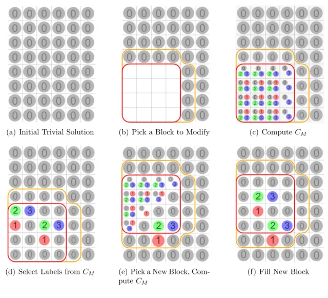
Algorithm 3.2 describes in detail how C is computed. Figure 3.4 shows an example of this computation. Figure 3.4(a) shows the example model. Suppose the size of M

is nx ×ny = 4×4. Initially, M0 is empty and CM0 contains all four possible labels in each of the 4×4 positions. Suppose that a 1’ label is assigned to a point in M as shown in Figure 3.4(b). That point is now reserved exclusively for the 1’ label. No