ffc61a547a76d602a882561b6967f39f8311841c.pdf

(1)

FIVE PLANETS TRANSITING A NINTH MAGNITUDE STAR

Andrew Vanderburg1,11, Juliette C. Becker2,11, Martti H. Kristiansen3,4, Allyson Bieryla1, Dmitry A. Duev5, Rebecca Jensen-Clem5, Timothy D. Morton6, David W. Latham1, Fred C. Adams2,7, Christoph Baranec8,

Perry Berlind1, Michael L. Calkins1, Gilbert A. Esquerdo1, Shrinivas Kulkarni5, Nicholas M. Law9, Reed Riddle5, Maïssa Salama10, and Allan R. Schmitt12

1

Harvard–Smithsonian Center for Astrophysics, 60 Garden Street, Cambridge, MA 02138, USA;[email protected]

2

Astronomy Department, University of Michigan, Ann Arbor, 48109, USA

3_{DTU Space, National Space Institute, Technical University of Denmark, Elektrovej 327, DK-2800 Lyngby, Denmark} 4

Brorfelde Observatory, Observator Gyldenkernes Vej 7, DK-4340 Tølløse, Denmark

5

California Institute of Technology, Pasadena, CA, 91125, USA

6

Department of Astrophysical Sciences, 4 Ivy Lane, Peyton Hall, Princeton University, Princeton, NJ 08544, USA

7

Physics Department, University of Michigan, Ann Arbor, 48109, USA

8

University of Hawai‘i at Mānoa, Hilo, HI 96720, USA

9

University of North Carolina at Chapel Hill, Chapel Hill, NC, 27599, USA

10

University of Hawai‘i at Mānoa, Honolulu, HI 96822, USA

Received 2016 May 2; accepted 2016 June 27; published 2016 August 4

ABSTRACT

TheKeplermission has revealed a great diversity of planetary systems and architectures, but most of the planets discovered byKepler orbit faint stars. Using new data from the K2 mission, we present the discovery of aﬁ ve-planet system transiting a bright(V=8.9,K=7.7)star called HIP41378. HIP41378 is a slightly metal-poor late F-type star with moderate rotation(vsini;7km s-1₎_{and lies at a distance of 116}__±__{18 pc from Earth. We}_ﬁ_nd

that HIP41378 hosts two sub-Neptune-sized planets orbiting 3.5% outside a 2:1 period commensurability in 15.6 and 31.7 day orbits. In addition, we detect three planets that each transit once during the 75 days spanned by K2 observations. One planet is Neptune-sized in a likely∼160 day orbit, one is sub-Saturn-sized, likely in a∼130 day orbit, and one is a Jupiter-sized planet in a likely∼1 year orbit. We show that these estimates for the orbital periods can be made more precise by taking into account dynamical stability considerations. We also calculate the distribution of stellar reﬂex velocities expected for this system, and show that it provides a good target for future radial velocity observations. If a precise orbital period can be determined for the outer Jovian planets through future observations, this system will be an excellent candidate for follow-up transit observations to study its atmosphere and measure its oblateness.

Key words:planets and satellites: detection– planets and satellites: gaseous planets

1. INTRODUCTION

The Kepler spacecraft (launched in 2009) has been a tremendously successful planet hunter (Borucki et al. 2010,2011; Koch et al.2010). Over the course of its original mission, which lasted four years,Keplerdiscovered thousands of planetary candidates around distant stars (Coughlin et al. 2016), demonstrating the diversity and prevalence of planetary systems (e.g., Muirhead et al. 2012; Orosz et al. 2012; Fabrycky et al. 2014; Morton & Swift2014).Kepler’s contributions include measuring the size distribution of exoplanets (Howard et al. 2012; Fressin et al.2013; Petigura et al. 2013b), understanding the composition of planets intermediate in size between the Earth and Neptune (Weiss & Marcy2014; Wolfgang et al.2016), measuring the prevalence of rocky planets in their host stars’habitable zones(Dressing & Charbonneau 2013, 2015; Petigura et al. 2013a; Foreman-Mackey et al. 2014; Burke et al. 2015), and uncovering the wide range of orbital architectures, such as tightly packed planetary systems (Campante et al. 2015), and planets in and

(more commonly) near low-order mean motion resonances

(MMRs; Carter et al.2012; Steffen & Hwang2015).

While Kepler’s discoveries have been illuminating, many questions about these systems still remain, and are difﬁcult to

answer because Kepler planet host stars are typically faint.

Kepler observed a single 110 square degreeﬁeld for 4 years, and that deep survey strategy produced many candidates that are too faint for intensive follow-up observations. Because of this limitation, our understanding of the properties of Kepler

planets is incomplete. For instance, radial velocity(RV) follow-ups of the brightest planet candidates on short period orbits have found that planets smaller than about 1.5 Earth radii are typically rocky(Dressing et al.2015; Rogers2015), but masses measured from the inversion of transit-timing variations

(TTVs) show a population of low-density planets orbiting farther from their host stars than most transiting planets with RV measurements (Steffen 2016). There are few planets with masses measured from TTVs transiting stars bright enough for RV follow-up, and in the few cases where both types of measurements are possible, there is not always perfect agreement (e.g., KOI 94: Masuda et al. 2013; Weiss et al. 2013).Keplerhas also discovered giant planets transiting stars on long-period orbits (Kipping et al. 2014, 2016) whose atmospheres could be studied via transmission spectroscopy

(Dalba et al. 2015), but these planets orbit stars fainter than most stars hosting planets with well-characterized atmospheres

(e.g., Deming et al.2013; Kreidberg et al.2014).

The end of the original Kepler mission in 2013 due to a mechanical failure has led to new opportunities for theKepler

spacecraft to discover planets orbiting brighter stars than

11

NSF Graduate Research Fellow.

12

(2)

before. In its new K2 extended mission (Howell et al. 2014),

Kepler observes manyﬁelds along the ecliptic plane for up to 80 days. Over the course of the K2 mission, Kepler could survey up to 20 times the sky area as it did in its original mission, greatly increasing the number of bright stars and other rare objects observed. The K2 mission has already yielded transiting planets and candidates around(for example)stars as bright as 8th magnitude (Vanderburg et al. 2016), nearby M-dwarfs (Crossﬁeld et al.2015; Petigura et al.2015; Hirano et al. 2016; Schlieder et al. 2016), and stars in nearby open clusters(Mann et al.2016).

Because it only observes stars for about 80 days before moving onto new ﬁelds, K2 is not as sensitive to planetary systems with complex architectures as the original Kepler

mission. While Kepler detected systems with up to seven transiting planets(Cabrera et al.2014; Schmitt et al.2014),K2

has not yet discovered any systems with more than three transiting planet candidates13(Sinukoff et al.2015; Vanderburg et al.2016).

In this paper, we report the discovery of a system of ﬁve transiting planets using K2 data. The host star is one of the brightest planet host stars from eitherKeplerorK2, with a V-magnitude of 8.9 and a K V-magnitude of 7.7, and has a trigonometric parallax-based distance of 116±18 pc. The planetary system displays a rich architecture, with two sub-Neptunes slightly outside of MMR and three larger planets in longer period orbits. The outer planet is a gas giant on an approximately 325 day orbit(detected by a single transit in the 80 days of K2 data), and if a precise orbital period can be recovered, it will be a favorable target for follow-up observations. In Section 2 we describe both the K2 observa-tions and our follow-up observaobserva-tions taken to characterize the system and rule out false positive scenarios. Section3presents our analysis and a determination of planet parameters, our statistical validation of the transit signals as genuine planets, and includes dynamical constraints requiring system stability. A discussion of our results is presented in Section4, followed by a summary in Section 5.

2. OBSERVATIONS

2.1. K2 Light Curve

HIP41378, also known as EPIC 211311380 and K2-93, was observed by theKeplerspace telescope during Campaign 5 of its extendedK2mission for a period of about 75 days between 2015 April 27 and 2015 July 10. We downloaded the calibrated target pixelﬁles for HIP41378 from the Mikulski Archive for Space Telescopes, and processed the light curve following Vanderburg & Johnson(2014)and Vanderburg et al.(2016)to produce a photometric light curve and remove systematic effects from the light curve caused by the K2 mission’s unstable pointing. Visual inspection of the K2 light curve by one of us (M.H.K.) revealed the presence of nine individual transit events at high conﬁdence. A Box Least Squares periodogram search (Kovács et al. 2002) of the light curve revealed that four of the nine individual transits occur periodically every 15.57 days. Two other transits are also consistent in shape, duration, and depth and occur approxi-mately 31.7 days apart, suggesting two planets near the 2:1 MMR. The remaining three transit events seen in the K2light

curve are not consistent with one another and each have longer durations than the repeating transits, suggesting orbital periods that are longer than the 75 days of K2 observations. We designateﬁve planet candidates around HIP41378; we refer to the inner two candidates as HIP41378b and HIP41378c, in order of increasing orbital period, and we refer to the outer three planet candidates as HIP41378d, HIP41378e, and HIP41378f, in order of increasing transit duration.

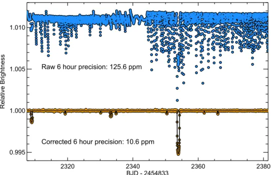
After identifying transits in the light curve, we reprocessed theK2 data by simultaneously ﬁtting the transits with theK2

roll systematics and the long-term variability in the star’s light curve, as described in Vanderburg et al.(2016). The resulting light curve has a precision of 10.6 parts per million(ppm)per six hours or 38 ppm per 30 minute long cadence exposure and is shown in Figure 1 along with the raw uncorrected light curve.

The photometric aperture we used to extract the K2 light curve is large due to HIP41378’s brightness. We inspected archival imaging from the Palomar Observatory Sky Survey and found that another nearby star that was about ﬁve magnitudes fainter than HIP41378 falls inside our photometric aperture. We checked that the transit signals are in fact centered on HIP41378 by extracting a light curve from smaller photometric apertures that exclude the nearby star. Although the photometric precision of the light curves from smaller apertures is signiﬁcantly worse than the photometric precision of our original large aperture, we detect all nine transits at the same depths as the original light curve. We therefore conclude that the transits are not centered on the fainter star.

2.2. High Resolution Spectroscopy

We observed HIP41378 with the Tillinghast Reﬂector Echelle Spectrograph(TRES)on the 1.5 m telescope at Fred L. Whipple Observatory on Mt. Hopkins, Arizona. We obtained spectra on four different nights in 2016 January and February. The spectra were obtained at a spectral resolving power of

λ/Δλ=44,000, and exposures of 360–450 s yielded spectra with signal-to-noise ratios of 90 to 110 per resolution element. We see no evidence for chromospheric calcium II emission from the H-line at 396.85 nm. We cross-correlated the four spectra with a model spectrum and inspected the resulting cross-correlation functions(CCFs). There is no evidence in the CCFs for additional, second sets of stellar lines. We measure an absolute RV for HIP41378 of 50.7km s-1_{, and the four}

individual spectra show no evidence for high-amplitude RV variations. We measured relative radial velocities by cross-correlating each observation with the strongest observation and found no evidence for RV variations greater than TRES’s intrinsic RV precision of 15m s-1_.

2.3. Adaptive Optics Imaging

We observed HIP41378 with the Robo-AO adaptive optics

(AO)system on the 2.1 m telescope at the Kitt Peak National Observatory(Baranec et al.2014; Law et al.2014; Riddle et al. 2016). Robo-AO is a robotic laser guide star adaptive optics system, which has recently moved to the 2.1 m telescope at Kitt Peak from the 1.5 m telescope at Palomar Observatory. We obtained an image on 2016 April 2 with ani′-bandﬁlter. The observation consisted of a series of exposures taken at a frequency of 8.6 Hz, which were then shifted and added using

13_{The WASP-47 system hosts four planets, only three of which are known to}

(3)

HIP41378 as the tip–tilt guide star. The total integration time was 120 s.

The resulting image showed no evidence for any compa-nions to HIP41378 within the 36″×36″ Robo-AO ﬁeld of view; the nearby star discussed in Section2.1falls outside the

ﬁeld of view. The AO observations allow us to exclude the presence of companion stars two magnitudes fainter than HIP41378 at a distance of 0 25, and stars four magnitudes fainter at a distance of 0 7 with 5σ conﬁdence.

3. ANALYSIS

3.1. Spectroscopic and Stellar Properties

We measured spectroscopic properties from each of the four TRES observations using the Stellar Parameter Classiﬁcation

(SPC, Buchhave et al. 2012, 2014) method. SPC cross-correlates observed spectra with a suite of synthetic spectra based on Kurucz (1992) atmosphere models, and interpolates the CCFs to determine the stellar effective temperature, metallicity, surface gravity, and projected rotational velocity. The four exposures yield consistent spectroscopic parameters, which are summarized in Table2. HIP41378 appears to be a slightly evolved late F-type star with a temperature of 6199±50 K, a surface gravity of loggcgs,SPC=4.13±0.1,

a metallicity[M/H]of−0.11±0.08, and a projected rotation velocity of 7.13±0.5km s-1_.

We determined the mass and radius of HIP41378 using an online interface14 to interpolate the star’s temperature, metallicity, V-band magnitude, and Hippacos parallax onto Padova stellar evolution tracks, as described by da Silva et al.

(2006). We ﬁnd that HIP41378 has a mass of 1.15±0.064M_e and a radius of 1.4±0.19R_e. The models predict a slightly stronger surface gravity of loggcgs=4.18±0.1 than the spectroscopic measurement of

4.13±0.1, but the surface gravities are consistent at the 1σ level. The consistency between the spectroscopic and model surface gravities provide an independent check that our stellar parameters are reasonable.

3.2. Transit Analysis

We analyzed theK2light curve by simultaneouslyﬁtting the

five transiting planet candidates and a model for low-frequency variability using a Markov Chain Monte Carlo algorithm with an affine invariant ensemble sampler (Goodman & Weare 2010). Wefit thefive transiting planet candidates with Mandel & Agol (2002) transit models, and we modeled the low frequency variations with a basis spline. For the two inner candidates, wefit for the orbital period, time of transit, scaled semimajor axis (a/R_å), orbital inclination, and planet-to-star radius ratio (RP/Rå). For the three outer candidates with only

one transit, wefit for the transit time, duration(from thefirst to fourth contact), transit impact parameter, and planet-to-star radius ratio. Wefit for quadratic limb darkening coefficients for all five transits simultaneously, using the the q1 and q2

parametrization from Kipping(2013a). We imposed no priors on these parameters other than requiring that impact parameters be positive. We accounted for the effects of the Kepler long cadence exposure time by oversampling each model data point by a factor of 30 and performing a trapezoidal numerical integration. We did not account for any asymmetry in the transit light curve due to eccentricity—this effect scales with

(a/R_å)−3and is too small to detect for long-period planets like these(Winn2010). We note that our choice to parameterize the orbits by their inclinations is an approximation—although orbits are uniformly distributed incosi, noti, the difference is negligible for nearly edge-on orbits like those of the planets transiting HIP41378. We performed a Monte Carlo calculation and found that the different parameterizations only change our Figure 1.RawK2light curve(blue, top), and systematic corrected light curve(orange, bottom). The best-fit transit model is shown as a black line over the orange systematics-corrected light curve. We haveflattened the light curve by removing our best-fit long term trend from the simultaneous transit/systematicfit. The three deepest transits are single-events, and are highly inconsistent with each other in terms of depth and duration. The systematics correction improves the photometric precision to a level of 10 ppm per six hours—comparable to the best light curves from the originalKeplermission.

14

(4)

ﬁnal measured inclinations by roughly 10−4degrees, much less than our measured uncertainties in inclination.

We sampled the parameter space using 150 walkers evolved through 40,000 links, and removed theﬁrst 20,000 links during which time the chains were“burning-in”to a converged state. This yielded a total of 3,000,000 individual samples. We tested the convergence of the MCMC chains by calculating the Gelman-Rubin statistic (Gelman & Rubin 1992). For each parameter, the Gelman-Rubin statistic was below 1.04, indicating our MCMC ﬁts wereconverged.

We plot the transit light curves for each planet and the

best-ﬁtting transit model in Figure2.

3.3. Statistical Validation

The transit signals in theK2 light curve of HIP41378 that we attribute to transiting planets could in principle have a non-planetary astrophysical origin. In this subsection, we argue that astrophysical false positive scenarios are unlikely in the case of the HIP41378 system, and a planetary interpretation of the transit signals is well justiﬁed.

We began by calculating the false positive probability(FPP) of the inner two planet candidates, which both have precisely measured orbital periods from multiple transits in the K2light curve, using the vespa software package (Morton 2012, 2015).Vespatakes information about the transit shape, orbital period, host star parameters, location in the sky, and observational constraints and calculates the likelihood that a given transit signal has an astrophysical origin other than a transiting planet. We used vespa to calculate the FPP of HIP41378b and HIP41378c given constraints on the depth

of any secondary eclipse from theK2light curve and limits on any nearby companion stars in theK2aperture from Robo-AO. We also used the fact that our RV measurements of HIP41378 show no variations greater than about 15m s-1_{to exclude all}

foreground eclipsing binary false positive scenarios. Given these constraints, we calculate that the FPP for HIP41378b is very small, of order 2×10−6, and the FPP of HIP41378c is 3×10−3, somewhat larger but still quite low. These FPPs do not take into account the fact that we detect ﬁve different candidate transit signals toward HIP41378 and that the vast majority ofKepler multi-transiting candidate systems are real planetary systems(Latham et al. 2011; Lissauer et al. 2012). Lissauer et al.(2012)estimate that being in a system of three or more candidates increases the likelihood of a given transit signal being real by a factor of ∼50–100. Taking this multiplicity argument into account, the FPP for HIP41378b decreases to roughly 10−7 and the FPP for HIP41378c decreases to roughly 10−4. We therefore consider HIP41378b and HIP41378c to be validated as genuine planets.

It is more difﬁcult to calculate the FPP for the outer planet candidates. Because the orbital period is unconstrained, a

(5)

periods. Lissauer et al.(2012)give expressions for estimating the likelihood of false positive signals in multiple planet systems. Using these expressions with numbers from the recent Data Release 24 Kepler planet candidate catalog (Coughlin et al.2016), wefind that the probability of a given target having two planets and three false positives is roughly 10−12, the probability of the target having three planets and two false positives is roughly 10−9, and the probability of the target having four planets and one false positive is roughly 5×10−7. From the observed number of systems with five or more transiting planets discovered byKepler, the probability of a star hosting such a system is roughly 18/198646 or 10−4. When we compare these probabilities, we find that, a priori, it is 108 times more likely that HIP41378 hosts five transiting planets than two planets and three false positives, 105times more likely that HIP41378 hostsfive transiting planets than three planets and two false positives, and about 200 times more likely that HIP41378 hosts five transiting planets than four planets and one false positive. When this information is combined with the fact that the transits are u-shaped(consistent with small planets) rather than v-shaped (consistent with a background false positive), and our adaptive optics imaging rules out many possible background contaminants, we have high confidence that all five candidates in the HIP41378 system are genuine planets.

3.4. Dynamics

The richness of the HIP41378 planetary system gives rise to questions about its dynamics and architecture. In this section, we aim to address and place constraints on the dynamical stability of the system and the resonance state of the inner two planets. The dynamical stability arguments we make in this section are useful for constraining the orbital periods of the outer two planets (which we do in Section3.5).

3.4.1. Inner Planets

Weﬁrst considered the two inner planets, which both show multiple transit events in theK2light curve and therefore have precisely measured orbital periods. The ratio of the orbital periods of the two inner planets is just 3.57% larger than 2:1, so we tested whether the two planets orbit in a 2:1 MMR.

We assessed the resonant state of the inner two planets by conducting 10,000 numerical simulations of the orbits of the inner two planets over 100,000 years using theMercury6N -body integrator (Chambers1999). For each trial, we drew the orbital elements of each planet from the posterior probability distribution from the MCMC transit ﬁt (Section 3.2). We assigned masses to the planets using the the methodology of Becker & Adams(2016)—to summarize, given the planet radii, we draw masses from several published mass–radius relations: the Weiss & Marcy (2014) relation for planets with

Rp<1.5R⊕, the Wolfgang et al. (2016) relation for planets with 4R_⊕>Rp>1.5R⊕, and for planets larger than 4R⊕we solve for mass by drawing the mean planetary density from a normal distribution centered at ρ=1.3±0.5 g cm−3, taking the hot Jupiter radius anomaly into account using the relation from Laughlin et al.(2011).

We tested each of the 10,000 realizations of the system for resonant behavior. The condition for resonance is more stringent than that of a period commensurability: for a pair of planets to be resonant, they must have oscillating(rather than

circulating)resonance angles, which means that the longitude of conjunction(the location where the the planets pass closest together)has an approximately stable location. Resonances are sometimes referred to as a“bound states”because planets can be trapped in the energetically favorable conﬁguration where the resonance angles oscillate back and forth in a potential well, like a pendulum with an energy low enough to swing back and forth rather than swing 360°over the top(Ketchum et al.2013). At the same time, a pair of planets can have a period ratio slightly out of an integer ratio and still be in resonance. We examined the resonance argument of the inner two planets,j, which is deﬁned as:

( ) ( )

j= p +q linner -plouter -qvouter, 1

wherep/(p+q)is the order of the resonance(which is 2:1, so

p=1 and q=1 for these planets), ϖ is the longitude of pericenter, andλis the angular location in orbit.

Out of the 10,000 system realizations that we tested, none of them were in resonance (all had circulating rather than oscillating resonant arguments). Therefore, we conclude that the inner two planets orbiting HIP41378 do not orbit in a MMR. This conclusion is not surprising—the sample of multi-planet systems fromKeplershows that planets more often orbit near, but not in, MMRs (Veras & Ford 2012). The fact that these planets orbit slightly outside of MMR is also reminiscent of trends seen inKeplermulti-planet systems. Fabrycky et al.

(2014)found that period ratios slightly larger than 2:1(as is the case for these two planets) are overrepresented in the population of observed systems, and slightly smaller ratios are underrepresented. Thus, there is no evidence to suggest that these planets are in resonance, but they are a part of the overabundance of planets that pile up slightly outside the 2:1 MMR.

We note that in this analysis, we have examined only the behavior of the two inner planets. The three outer planets in the system contribute additional terms in Equation (1), which we have ignored because of their poorly constrained orbits, but which could presumably alter the resonant behavior of the inner two planets. However, we believe that it is unlikely that the outer planets would signiﬁcantly affect the inner planets’ resonant state. The periods of the outer three planets are likely signiﬁcantly longer (by an order of magnitude or so, see Section 3.5)than the periods of the inner two planets, so the outer planets will act like distant static perturbers.

3.4.2. Outer Planets

We performed a separate dynamical analysis to study possible orbits and conﬁgurations of the outer three planets in the HIP41378 system. The outer three planets only transited HIP41378 once during the 75 days ofK2observations, so their orbital periods are not uniquely determined from the light curve. We do, however, measure the transit duration, radius ratio, and impact parameter of the three single-transit events, and our follow-up spectroscopy and analysis measures the mean stellar density, which allows us to estimate the semimajor axes and orbital periods of the three outer planets(see Table2 for the best-ﬁt values for each parameter).

(6)

We estimated the outer singly transiting planets’ orbital periods (and therefore semimajor axes) from the transit and stellar parameters using an analytical expression (e.g., Seager & Mallén-Ornelas 2003) with a correction for nonzero eccentricity(as in Ford et al.2008):

( )

( ) ( ) ] ( )

*

* *

p p

v

= +

´ + - ´

-+

-⎡

⎣ ⎢ ⎢ ⎛ ⎝

⎜ ⎞

⎠ ⎟

t P G M m P

R R b R e

e arcsin

4

1

1 cos , 2

d i

i p i i

P i i

i

i i

,

, 2

2

1 3

, 2 2 2

2

where td,iis the transit duration of theith planet(fromﬁrst to fourth contact), Pi is its period (for which we would like to solve), mp,i is the mass of the ith planet, ei is the orbital eccentricity, ϖiis the argument of periastron, bi is the impact parameter,M_*is the stellar mass,R_*is the stellar radius, andG

is the gravitational constant.

We solved Equation (2) numerically 4000 times for each outer planets’ orbital period (which we then converted to semimajor axis). For each of the 4000 realizations, we drew the quantities td,i, Pi,RP,i, and bi from the light curve posterior probability distributions from the MCMC transit ﬁts. We generated the planet massesmp,ifrom the measured planet radii using the same piecewise mass–radius relation as was used in 3.4.1. Values for M_* and R_* were drawn from the posterior probability distributions generated in Section 3.1, and values for e were drawn from a beta distribution with shape parameters α=0.867 and β=3.03 (derived from the population of observed planets given in Kipping 2013b, 2014; Kipping & Sandford 2016). We used an asymmetric prior for the argument of periastronϖ to account for the fact that the planet is observed to be transiting(the value of which is dependent on the drawn eccentricity; see Equation (19) in Kipping & Sandford2016).

After determining initial parameters, we integrated each of the 4000 systems forward in time for 1 Myr, long enough to examine interactions over many secular periods, while requiring energy be conserved to one part in 108. Of the total 4000 realizations, only a subset (roughly 10%) were dynami-cally stable over 1 Myr timescales, meaning that dynamical arguments can help constrain the system architecture, including the orbits of the three outer planets. We found that the most important variables for determining the stability of the system

are the orbital eccentricities of the individual planets. For a given transit duration, the orbital period and eccentricity are degenerate. As a result, the eccentricities’constraints translate into limits on the orbital periods of the outer planets.

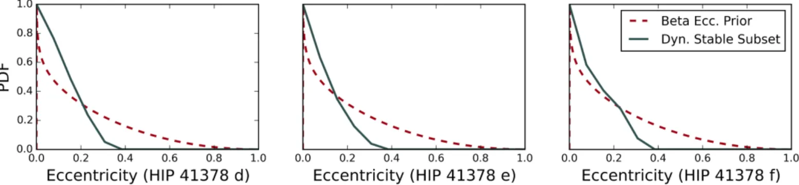
Figure 3 shows the difference in initial eccentricity distribution (namely, the beta distribution prior) and the eccentricity distribution of the planets in systems that remained dynamically stable. These distributions are visibly different, and the eccentricities of stable systems are preferentially lower. Among our 4000 realizations, all systems containing planets with eccentricities above e∼0.37 became dynamically unstable, suggesting that the true eccentricities are less than this value.

3.5. Orbital Periods of the Outer Planets

In this section, we estimate the orbital period of the three outer planets transiting HIP41378 under various assumptions and taking different information into account. We calculate orbital periods with a similar analysis to that described in the previous section, in particular by solving Equation (2) numerically after drawing parameters from the MCMC transit

ﬁt posterior probability distributions or from priors.

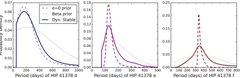
Wefirst calculated orbital periods under the assumption of strictly circular orbits. We also required that the orbital periods be longer than the baseline ofK2observations before and after each event—otherwise we would have seen multiple transits. We find that when we assume a circular orbit, we obtain relatively tight limits on the periods of the outer three planets, in particular the two deepest transits with precisely measured durations and impact parameters. For long-period planets like these, however, the assumption of a circular orbit is in general not justified, so we believe these orbital period estimates are artificially tight. The distributions of orbital periods for the outer three planets assuming circular orbits are shown in Figure4.

We also calculated orbital periods with the assumption of circular orbits relaxed to allow orbital eccentricities and arguments of periastron drawn from the same beta distribution and asymmetric prior described in the previous section (and which we used as an input to the dynamical simulations). As noted previously, this distribution matches the observed distribution of orbital eccentricity for exoplanets detected by radial velocities. When we do not assume circular orbits, the limits on the orbital periods are much looser. Although the median orbital periods we derived under the assumption of Figure 3.Comparison of input planet eccentricity to dynamical simulations(red dashed lines)and the eccentricity of planets in dynamically stable systems(black solid lines). The input to the dynamical simulations is the distribution of eccentricities in all exoplanets detected with radial velocities(Kipping2013b). The difference in shape between the two curves demonstrates which eccentricities are preferred in dynamically stable systems. Evidently, planets with eccentricities larger than

(7)

circular orbits and eccentric orbits are relatively similar, the width of the distribution changes drastically. In the case of HIP41378f, the uncertainty on the orbital period increases by an order of magnitude when taking into account nonzero eccentricity. The orbital period distributions given this prior on orbital eccentricity are also shown in Figure4, where they can be compared to the case of circular orbits.

The fact that the eccentricity of exoplanets tends to follow a beta distribution is not the only information we have about the system architecture or orbital eccentricities of the outer three planets. We can place additional constraints on the orbital eccentricities (and therefore orbital periods) by requiring that the system be dynamically stable. In Section 3.4.2, we found that the HIP41378 system is dynamically unstable on 1 Myr timescales when any of the planets have eccentricities greater than 0.37, so we remove all orbital periods with eccentricities greater than 0.37. We also remove all systems that are not Hill stable (using the criterion from Fabrycky et al. 2014). Enfor-cing these dynamical stability criteria narrows the distributions of plausible orbital periods by about 30%. The orbital period distributions with dynamical stability enforced are also shown in Figure 4, along with distributions without dynamical stability enforced for comparison.

Finally, we took into account the fact that we observed these three planets to be transiting during the 75 days of K2

observations. Planets with shorter orbital periods are more likely to transit during a limited baseline than planets with longer orbital periods. We take this information into account by imposing a prior of the form:

( ) ₍ ₎ ( )

 =⎪ ₊ - <

⎪

⎧ ⎨ ⎩ P t B

P t B

B t P

, , 1 if _else, 3

i d i

d i i

,

, ,

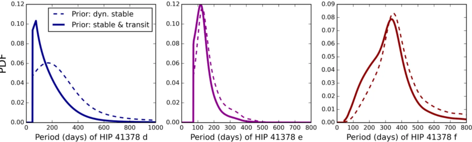
whereis the probability of observing a transit of planeti,Bis the time baseline of the observations, td,i is the ith planet’s transit duration, andPiis the orbital period of the planeti. Here, we deﬁne the planet being“observed to transit”as any part of its ingress or egress occurring during K2 observations. We imposed this prior on the orbital period distribution, taking into account nonzero orbital eccentricity and dynamical stability, and we show the result in Figure5. The effect of this prior is to narrow the period distributions by another ∼30% and to shift

the period distributions to slightly lower values. The effect is most pronounced on the period distribution of HIP41378d that had a weakly constrained orbital period because of its shallow transit.

We summarize our orbital period estimates under these various assumptions in Table1. We report the median values and 1σwidths of each distribution. In this paper, we choose to adopt the period distributions, which were calculated by taking into account nonzero eccentricity, dynamical stability, and the fact that the planets transiting during theK2observations as our best estimate for the outer planets’ orbital periods. These distributions incorporate the most information we have about the system to give the best possible period estimates.

4. DISCUSSION

HIP41378 is a compelling candidate for follow-up observa-tions due to its brightness, the accessible size of the planets, and the system’s rich architecture. HIP41378 is the second brightest multi-transiting system, behind Kepler-444

(Campante et al.2015), a system ofﬁve sub-Earth-sized planets with expected RV semi-amplitudes below the noise-ﬂoor of current instrumentation. Unlike the Kepler-444 system, the planets orbiting HIP41378 should each have measurable RV semi-amplitudes. We have estimated the likely range of RV semi-amplitudes for each planet, assuming planetary masses drawn from the Wolfgang et al.(2016)distribution and periods and eccentricities drawn from our analysis in Sections3.4.2and 3.5. The RV semi-amplitude distributions, shown in Figure6, are all centered above 1 m s-1_{, and could therefore be}

detectable with spectrographs like HARPS-N (Cosentino et al. 2012) and HIRES (Vogt et al. 1994) in the north, and HARPS(Mayor et al.2003)and PFS(Crane et al.2010)in the south. It will be the most challenging to detect HIP41378d, which has an unknown period (unlike the inner two planets) and most likely induces an RV semi-amplitude of only 2m s-1_,

but such signals have been detected previously in intensive observing campaigns(e.g., Lovis et al.2011).

(8)

originally present might have been stripped by the intense stellar radiation. Planet masses measured from transit-timing variations have shown that some planets on longer periods are likely less dense than most short period planets. Measuring precise masses of planets in longer period orbits(like the inner two planets in this system) can help show whether or not a planet’s radiation environment affects its density.

RV measurements will also be important for determining the orbital period of the outer planets, in particular the long-period gas giant HIP41378f. This planet’s long orbital period and the brightness of the host star make HIP41378f a promising target for future transit follow-up studies—provided a precise orbital period and transit ephemeris can be recovered. HIP41378 is

ﬁve magnitudes brighter than the recently discovered transiting Jupiter analog host Kepler-168 (Kipping et al. 2016), making HIP41378f one of the best long-period transiting planets for transit transmission spectroscopy. Studying HIP41378f’s atmosphere will open up a new regime for atmospheric studies, which typically focus on short period, highly irradiated planets. HIP41378f could also be a compelling target to measure the planet’s oblateness. The planets in our own solar system are not spherical and are distorted into oblate spheroids by the planets’ rotation. A planet’s projected oblateness can be measured from its transit light curve (Hui & Seager 2002). Indeed, strong constraints have been placed on the degree of oblateness for hot Jupiters (Carter & Winn 2010; Zhu et al. 2014), even though these planets are not expected to show measurable oblateness because their rotation periods are likely to be synchronized with their orbits(Seager & Hui2002). The long period of HIP41378f implies that its rotation will not

have tidally synchronized with its orbit, so its oblateness is likely to be large enough to detect.

Follow-up observations of HIP41378f hinge on our ability to recover a precise orbital period and transit ephemeris. Because of the planet’s(apparent) long orbital period, it may be difﬁcult to measure the spectroscopic orbit precisely enough to recover transits using a non-dedicated instrument like Spitzer. The

CHEOPS spacecraft (Broeg et al. 2013) may be the ideal instrument to recover transit ephemerides for the outer planets

(and therefore precise orbital periods), given the mission focus on transiting planets. Long-term monitoring withCHEOPSmay also reveal additional transiting planet candidates with long orbital periods that did not happen to transit during theK2observations. The challenges we face attempting to measure precise orbital periods for planets with just a single transit in the HIP41378 light curve are not unique to this system. Numerous single-transits have been observed in both Kepler data(Wang et al. 2015) and K2 data (Vanderburg et al. 2015; Osborn et al. 2016). Previous studies(Yee & Gaudi2008; Wang et al.2015; Osborn et al.2016)have shown that it is possible to make sharp predictions of the orbital period of a planet with a single transit, assuming strictly circular orbits. This assumption is in general not justiﬁed for long-period exoplanets, where RV surveys have shown that high eccentricities (greater than those observed in our solar system) are common (Kipping 2013b), and weakly constrained eccentricity substantially increases the range of possible orbital periods(Yee & Gaudi2008). Here, we are able to take orbital eccentricity into account and still obtain relatively strong constraints on orbital periods by incorporating priors on eccentricity(from RV planet detections), dynamically stability, and detecting transits during the timespan of K2

Figure 5.Probability distributions for the orbital period of each of the single-transit planets in the system, incorporating dynamical stability alone(dashed lines)and incorporating dynamical stability and the probability of detecting a single transit withK2(solid lines). The distribution seen if only taking into account dynamical stability is the same as the solid lines shown in Figure4. Incorporating the prior information that these three planets transited duringK2observations sharpens our predictions of the orbital periods of the three outer planets.

Table 1

Estimated Periods for the Three Outer Planets using Four Choices of Priors

Eccentricity Prior HIP41378d Period HIP41378e Period HIP41378f Period

e=0 157-+41195 132-+1437 348-+1337

ebeta distribution(as used in Section3.4.2) 188-+39787 143-+52129 367-+130311 ebeta distribution, dynamically stable only 174-+68260 140-+4392 361-+103182 Adopted: ebeta distribution, dyn. stable only+baseline prior 156-+78163 131-+3661 324-+127121

(9)

observations. These techniques should be developed further. In future work, they will provide valuable tools for estimating periods and other orbital elements for singly transiting planets in multi-planet systems fromKepler,K2, or TESS(Ricker et al. 2015), which will observe most of the sky for only 28 days and will likely discover over 100 planets with a single-transit event

(Sullivan et al.2015).

5. SUMMARY

Using data from the K2 mission, we have discovered, validated, and characterized the HIP41378 planetary system. Our main results can be summarized as follows.

1. HIP41378 hosts a system of at least ﬁve transiting planets, three of which were discovered by observing Table 2

System Parameters for HIP41378

Parameter Value 68.3% Conﬁdence Comment

Interval Width

Stellar Parameters

R.A. 8:26:27.85

decl. +10:04:49.35

Distance to Star[pc] 116 ± 18 A

V-magnitude 8.93 A

Må[Me] 1.15 ± 0.064 C

Rå[Re] 1.4 ± 0.19 C

Limb darkeningq1 0.311 ± 0.048 D

Limb darkeningq2 0.31 ± 0.13 D



g

log [cgs] 4.18 ± 0.1 C

Metallicity[M/H] −0.11 ± 0.08 B

Teff[K] 6199 ± 50 B

HIP41378b

Orbital Period,P[days] 15.5712 ± 0.0012 D

Radius Ratio,(RP R) 0.0188 ± 0.0011 D

Scaled semimajor axis,a/Rå 19.5 ± 4.5 D

Orbital inclination,i[deg] 88.4 ± 1.6 D

Transit impact parameter,b 0.55 ± 0.28 D

Time of Transittt[BJD] 2457152.2844 ± 0.0021 D

RP[R⊕] 2.90 ± 0.44 C, D

HIP41378c

Orbital Period,P[days] 31.6978 ± 0.0040 D

Scaled semimajor axis,a/Rå 73 ± 18 D

Orbital Inclination,i[deg] 89.58 ± 0.52 D

Transit Impact parameter,b 0.53 ± 0.29 D

RP[R⊕] 2.56 ± 0.40 C, D

HIP41378d

Orbital Period,P[days] 156-+78163 E

Transit Impact Parameter,b 0.50 ± 0.27 D

Transit DurationD[hours] 12.71 ± 0.26 D

RP[R⊕] 3.96 ± 0.59 C, D

HIP41378e

RP[R⊕] 5.51 ± 0.77 C, D

HIP41378f

Radius Ratio,(RP/Rå) 0.0672 ± 0.0013 D

RP[R⊕] 10.2 ± 1.4 C, D

(10)

(only)a single transit. The two inner planets, in 15.6 and 31.7 day orbits, have radii RP=2.9 and 2.6 R⊕, respectively. The three single-transit planets have radii of RP=4, 5.5, and 10 R⊕, and orbital periods that are likely longer than 100 days. These planets orbit a particularly bright F-type star, HIP41378. The host HIP41378 is a slightly evolved F-star with a V-band magnitude of 8.9, an H-band magnitude of 7.8, and a K-band magnitude of 7.7. As a result, its planetary system is a good candidate for follow-up observations. 2. The outer three planets only transited HIP41378 once

during the 75 days ofK2 observations. Although orbital periods are not well-deﬁned for single - transit events, we have constrained the orbital periods of the newly discovered planets. Using our knowledge of the host’s stellar properties and the planets’transit parameters, and a reasonable prior on the orbital eccentricity, we estimate a range of possible orbital periods for the outer three planets. We are able to sharpen these estimates by a factor of two by incorporating information about the system’s dynamical stability and the probability of a transit being observed during the K2 observations. We ﬁnd that the most likely periods for the three new planets are156-+78163,

-+

131 36 61

, and 324-+126 121

days for planets d, e, and f, respectively.

3. Follow-up RV observations could measure masses for all of the planets and could determine orbital periods for the three outer planets. We calculate that the reﬂex velocities on HIP41378 from HIP41378b, HIP41378c, and HIP41378d are likely to fall in the range 2–4m s-1_{, and}

thus are detectable with current instrumentation. The two inner planets have known periods, which will aid in isolating the RV signals of the outer planets. HIP41378e and HIP41378f have expected reﬂex velocities of approximately 5 and 25 m s−1, respectively, and should be readily detectable with enough observational coverage.

4. HIP41378f is a gas giant in a likely 1 year orbit. The host star’s brightness and HIP41378f’s 0.5% transit depth make it an attractive target for future transit follow-up observations if its precise orbital period and transit ephemeris can be recovered. HIP41378f is one of the

ﬁrst gas giants with a cool equilibrium temperature transiting a star bright enough for transit transmission spectroscopy. It could also be possible to measure the planet’s oblateness, since its orbital period is long enough that its rotation will not have synchronized with its orbit.

Discoveries such as the HIP41378 system show the value of wide-field space-based transit surveys. TheKepler spacecraft had to search almost 800 square degrees of sky(or sevenfields of view) before finding such a bright multi-planet system suitable for follow-up observations. HIP41378 is a preview of the type of discoveries the all-sky TESS survey will make routine.

We thank the anonymous referee for helpful comments on the manuscript. A.V. and J.C.B. are supported by the NSF Graduate Research Fellowship, grants No. DGE 1144152 and DGE 1256260, respectively. D.W.L. acknowledges partial support from the Kepler mission under NASA Cooperative Agreement NNX13AB58A with the Smithsonian Astrophysi-cal Observatory. C.B. acknowledges support from the Alfred P. Sloan Foundation.

This research has made use of NASA’s Astrophysics Data System and the NASA Exoplanet Archive, which is operated by the California Institute of Technology, under contract with the National Aeronautics and Space Administration under the Exoplanet Exploration Program. This work used the Extreme Science and Engineering Discovery Environment (XSEDE), which is supported by National Science Foundation grant number ACI-1053575. This research was done using resources provided by the Open Science Grid, which is supported by the National Science Foundation and the U.S. Department of Energy’s Ofﬁce of Science. The National Geographic Society– Palomar Observatory Sky Atlas (POSS-I) was made by the California Institute of Technology with grants from the National Geographic Society. The Oschin Schmidt Telescope is operated by the California Institute of Technology and Palomar Observatory.

This paper includes data collected by the Kepler mission. Funding for the Kepler mission is provided by the NASA Science Mission directorate. Some of the data presented in this paper were obtained from the Mikulski Archive for Space Telescopes(MAST). STScI is operated by the Association of Universities for Research in Astronomy, Inc., under NASA contract NAS5–26555. Support for MAST for non–HSTdata is provided by the NASA Ofﬁce of Space Science via grant NNX13AC07G and by other grants and contracts.

(11)

National Science Foundation under grants AST-0906060, AST-0960343, and AST-1207891, the Mt. Cuba Astronomical Foundation, and by a gift from Samuel Oschin. Based in part on observations at Kitt Peak National Observatory, National Optical Astronomy Observatory(NOAO Prop. ID: 15B-3001), which is operated by the Association of Universities for Research in Astronomy(AURA)under cooperative agreement with the National Science Foundation.

Facilities: Kepler/K2, FLWO:1.5 m(TRES), KPNO:2.1 m

(Robo-AO).

REFERENCES

Baranec, C., Riddle, R., Law, N. M., et al. 2014,ApJL,790, L8 Becker, J. C., & Adams, F. C. 2016,MNRAS,455, 2980

Becker, J. C., Vanderburg, A., Adams, F. C., Rappaport, S. A., & Schwengeler, H. M. 2015,ApJL,812, L18

Borucki, W. J., Koch, D., Basri, G., et al. 2010,Sci,327, 977 Borucki, W. J., Koch, D. G., Basri, G., et al. 2011,ApJ,736, 19 Broeg, C., Fortier, A., Ehrenreich, D., et al. 2013,EPJWC,47, 03005 Buchhave, L. A., Bizzarro, M., Latham, D. W., et al. 2014,Natur,509, 593 Buchhave, L. A., Latham, D. W., Johansen, A., et al. 2012,Natur,486, 375 Burke, C. J., Christiansen, J. L., Mullally, F., et al. 2015,ApJ,809, 8 Cabrera, J., Csizmadia, S., Lehmann, H., et al. 2014,ApJ,781, 18 Campante, T. L., Barclay, T., Swift, J. J., et al. 2015,ApJ,799, 170 Carter, J. A., Agol, E., Chaplin, W. J., et al. 2012,Sci,337, 556 Carter, J. A., & Winn, J. N. 2010,ApJ,709, 1219

Chambers, J. E. 1999,MNRAS,304, 793

Cosentino, R., Lovis, C., Pepe, F., et al. 2012,Proc. SPIE,8446, 84461V Coughlin, J. L., Mullally, F., Thompson, S. E., et al. 2016,ApJS,224, 12 Crane, J. D., Shectman, S. A., Butler, R. P., et al. 2010,Proc. SPIE,7735,

773553

Crossﬁeld, I. J. M., Petigura, E., Schlieder, J. E., et al. 2015,ApJ,804, 10 da Silva, L., Girardi, L., Pasquini, L., et al. 2006,A&A,458, 609 Dalba, P. A., Muirhead, P. S., Fortney, J. J., et al. 2015,ApJ,814, 154 Deming, D., Wilkins, A., McCullough, P., et al. 2013,ApJ,774, 95 Dressing, C. D., & Charbonneau, D. 2013,ApJ,767, 95

Dressing, C. D., & Charbonneau, D. 2015,ApJ,807, 45

Dressing, C. D., Charbonneau, D., Dumusque, X., et al. 2015,ApJ,800, 135 Fabrycky, D. C., Lissauer, J. J., Ragozzine, D., et al. 2014,ApJ,790, 146 Ford, E. B., Quinn, S. N., & Veras, D. 2008,ApJ,678, 1407

Foreman-Mackey, D., Hogg, D. W., & Morton, T. D. 2014,ApJ,795, 64 Fressin, F., Torres, G., Charbonneau, D., et al. 2013,ApJ,766, 81 Gelman, A., & Rubin, D. B. 1992, StaSc, 457, 457

Goodman, J., & Weare, J. 2010,Commun. Appl. Math. Comput. Sci., 5, 65 Hellier, C., Anderson, D. R., Collier Cameron, A., et al. 2012,MNRAS,426, 739 Hirano, T., Fukui, A., Mann, A. W., et al. 2016,ApJ,820, 41

Howard, A. W., Marcy, G. W., Bryson, S. T., et al. 2012,ApJS,201, 15 Howell, S. B., Sobeck, C., Haas, M., et al. 2014,PASP,126, 398 Hui, L., & Seager, S. 2002,ApJ,572, 540

Ketchum, J. A., Adams, F. C., & Bloch, A. M. 2013,ApJ,762, 71 Kipping, D. M. 2013a,MNRAS,435, 2152

Kipping, D. M. 2013b,MNRAS,434, L51 Kipping, D. M. 2014,MNRAS,444, 2263

Kipping, D. M., & Sandford, E. 2016, MNRAS, in press(arXiv:1603.05662) Kipping, D. M., Torres, G., Buchhave, L. A., et al. 2014,ApJ,795, 25 Kipping, D. M., Torres, G., Henze, C., et al. 2016,ApJ,820, 112 Koch, D. G., Borucki, W. J., Basri, G., et al. 2010,ApJL,713, L79 Kovács, G., Zucker, S., & Mazeh, T. 2002,A&A,391, 369 Kreidberg, L., Bean, J. L., Désert, J.-M., et al. 2014,ApJL,793, L27 Kurucz, R. L. 1992, in Proc. IAU Symp. 149, The Stellar Populations of

Galaxies, ed. B. Barbuy & A. Renzini(Dordrecht: Kluwer Academic),225 Latham, D. W., Rowe, J. F., Quinn, S. N., et al. 2011,ApJL,732, L24 Laughlin, G., Crismani, M., & Adams, F. C. 2011,ApJL,729, L7 Law, N. M., Morton, T., Baranec, C., et al. 2014,ApJ,791, 35 Lissauer, J. J., Marcy, G. W., Rowe, J. F., et al. 2012,ApJ,750, 112 Lovis, C., Ségransan, D., Mayor, M., et al. 2011,A&A,528, A112 Mandel, K., & Agol, E. 2002,ApJL,580, L171

Mann, A. W., Gaidos, E., Mace, G. N., et al. 2016,ApJ,818, 46

Masuda, K., Hirano, T., Taruya, A., Nagasawa, M., & Suto, Y. 2013,ApJ, 778, 185

Mayor, M., Pepe, F., Queloz, D., et al. 2003, Msngr,114, 20 Morton, T. D. 2012,ApJ,761, 6

Morton, T. D. 2015, VESPA: False Positive Probabilities Calculator, Astrophysics Source Code Library, ascl:1503.011

Morton, T. D., & Swift, J. 2014,ApJ,791, 10

Muirhead, P. S., Johnson, J. A., Apps, K., et al. 2012,ApJ,747, 144 Neveu-VanMalle, M., Queloz, D., Anderson, D. R., et al. 2016, A&A,

586, A93

Orosz, J. A., Welsh, W. F., Carter, J. A., et al. 2012,Sci,337, 1511 Osborn, H. P., Armstrong, D. J., Brown, D. J. A., et al. 2016, MNRAS,

457, 2273

Petigura, E. A., Howard, A. W., & Marcy, G. W. 2013a, PNAS, 110, 19273

Petigura, E. A., Marcy, G. W., & Howard, A. W. 2013b,ApJ,770, 69 Petigura, E. A., Schlieder, J. E., Crossﬁeld, I. J. M., et al. 2015,ApJ,811, 102 Ricker, G. R., Winn, J. N., Vanderspek, R., et al. 2015,JATIS,1, 014003 Riddle, R. L., Baranec, C., Law, N. M., et al. 2016, BAAS,227, 427.03 Rogers, L. A. 2015,ApJ,801, 41

Schlieder, J. E., Crossﬁeld, I. J. M., Petigura, E. A., et al. 2016,ApJ,818, 87 Schmitt, J. R., Wang, J., Fischer, D. A., et al. 2014,AJ,148, 28

Seager, S., & Hui, L. 2002,ApJ,574, 1004

Seager, S., & Mallén-Ornelas, G. 2003,ApJ,585, 1038

Sinukoff, E., Howard, A. W., Petigura, E. A., et al. 2015, ApJ, in press (arXiv:1511.09213)

Steffen, J. H. 2016,MNRAS,457, 4384

Steffen, J. H., & Hwang, J. A. 2015,MNRAS,448, 1956

Sullivan, P. W., Winn, J. N., Berta-Thompson, Z. K., et al. 2015, ApJ, 809, 77

Vanderburg, A., & Johnson, J. A. 2014,PASP,126, 948

Vanderburg, A., Latham, D. W., Buchhave, L. A., et al. 2016,ApJS,222, 14 Vanderburg, A., Montet, B. T., Johnson, J. A., et al. 2015,ApJ,800, 59 Veras, D., & Ford, E. B. 2012,MNRAS,420, L23

Vogt, S. S., Allen, S. L., Bigelow, B. C., et al. 1994, Proc. SPIE,2198, 362 Wang, J., Fischer, D. A., Barclay, T., et al. 2015,ApJ,815, 127

Weiss, L. M., & Marcy, G. W. 2014,ApJL,783, L6

Weiss, L. M., Marcy, G. W., Rowe, J. F., et al. 2013,ApJ,768, 14 Winn, J. N. 2010, arXiv:1001.2010

Wolfgang, A., Rogers, L. A., & Ford, E. B. 2016,ApJ,825, 19 Yee, J. C., & Gaudi, B. S. 2008,ApJ,688, 616