5977.pdf

(1)

Abrupt changes and intervening oscillations in conceptual

climate models

Andrew Roberts

A dissertation submitted to the faculty of the University of North Carolina at Chapel Hill in partial fulfillment of the requirements for the degree of Doctor of

Philosophy in the Department of Mathematics. Chapel Hill

2014

Approved by:

Christopher K.R.T. Jones Patrick Eberlein

(2)

(3)

ABSTRACT

ANDREW ROBERTS: Abrupt changes and intervening oscillations in conceptual climate models

(Under the direction of Christopher K.R.T. Jones)

(4)

(5)

ACKNOWLEDGEMENTS

(6)

LIST OF FIGURES

1.1. Oxygen isotope data from Greenland (NGRIP) . . . 5

1.2. Temperature record depicting interglacial periods . . . 6

1.3. Temperature record depicting the Mid-Pleistocene transition . . . 7

1.4. Relaxation Oscillation . . . 12

2.1. Example of a ‘2’ shaped critical manifold. . . 18

2.2. Fast and slow dynamics leading to canard explosion in the smooth case. 20 2.3. Examples of the three types of singular canard cycles . . . 22

2.4. Depiction of the quasi-canard explosion. . . 31

2.5. Relative slopes of vectors as discussed in the proof of Lemma 2.3.1. . . . 35

2.6. The setV for a given λ . . . 37

2.7. Images characterizing a nonsmooth canard explosion for = 0.2 . . . 38

2.8. An example of a setW which is positively invariant . . . 40

2.9. The stable orbit of a super-explosion (blue) for = 0.2 . . . 42

2.10. Positively invariant sets . . . 43

2.11. Important sets for the proof of Proposition 2.3.8 . . . 46

3.1. Oxygen isotope data from Greenland (NGRIP) . . . 51

3.2. Graphs of (3.6) for (a) A <1 and (b) A >1. . . 54

3.3. Bifurcation diagram for (3.4) . . . 55

3.4. Possible phase spaces of (3.10) for A <1 and 1 +a6=b . . . 58

3.5. Oscillatory behavior in (3.12). . . 61

3.6. Example of a singular periodic orbit . . . 66

3.7. Existence of a stable singular periodic orbit . . . 67

3.8. Regions of phase space that satisfy conditions (a)-(e). . . 74

(10)

4.1. Temperature record depicting interglacial periods . . . 79

4.2. Energy balance . . . 84

4.3. Cubic approximation of (4.10) . . . 87

4.4. Example of a singular periodic orbit . . . 92

4.5. A lower bound for the edge of the funnel. . . 98

4.6. Locally invariant regions on the critical manifold . . . 102

4.7. Parameters that will produce an MMO orbit . . . 106

4.8. MMO orbit . . . 107

4.9. More parameters that could produce MMOs . . . 108

4.10. Examples of MMO patterns in the three time-scale case. . . 109

(11)

CHAPTER 1

Introduction

1.1. Overview

Different mechanisms affect the Earth’s climate on very different time scales: from the 5-year El Ni˜no cycles, to the Atlantic Multidecadal Oscillation, to the Mi-lankovitch cycles with periods on the order of 10 millennia. Dynamical systems with variables that change on dramatically different time scales are called fast/slow systems. This thesis examines the role of fast/slow dynamics in understanding the mechanisms behind oscillatory patterns found in paleoclimate data. The intuitive approach to analyzing systems with multiple time scales is to analyze the dynamics on each time scale separately. In doing so, the fast dynamics may be attracted to an apparent equilibrium, however the equilibrium can be destabilized by the slow dynamics. Because full fast/slow system remains in this state for a long time, it is called a metastable state. Fast/slow systems often exhibit rapid transitions be-tween metastable states, and understanding these transitions is important in climate science. However, these rapid changes in the state of the system implicitly require ex-amining trajectories that enter a region of phase space where the basic theory used to analyze fast/slow systems no longer applies. The content of this thesis examines the non-standard behavior arising from the break down of the theory, typically appearing in the form of small amplitude oscillations.

(12)

Chapter 2 focuses on special behavior, called canard phenomena, in piecewise-smooth, planar systems, demonstrating conditions under which a piecewise-smooth, planar system exhibits small oscillations called canard cycles. Additionally, the dynamics are analyzed in the event that the conditions for canard cycles are not met, show-ing the existence ofsuper-explosion behavior in piecewise-smooth, nonlinear systems. Chapter 3 applies the results of Chapter 2 to a large-scale ocean circulation model that reduces to a system with 1 fast and 1 slow variable. A more complicated model with 1 fast and 2 slow variables is also analyzed, examining the consequences of a cusp catastrophe in large-scale ocean circulation. Chapter 4 explores the role of fast/slow dynamics in glacial-interglacial cycles of the past 400,000 years (400 kyr). A smooth model with 1 fast and 2 slow variables is analyzed, showing the existence of mixed-mode oscillations due to a generalized canard phenomenon. Chapter 5 summarizes the work of the previous chapters and discusses future directions of research.

1.2. Oscillations in Climate Data

(13)

to the varying parameter. That is, a large variation in the parameter can lead to a small change in the dynamics.

Nonlinear dynamical systems techniques, especially those designed to analyze sys-tems with multiple time scales, can be particularly effective in providing an under-standing of how feedback mechanisms function. Crucifix [12] surveys applications of these techniques to conceptual paleoclimate models, emphasizing oscillations in the climate system that can be seen as stable periodic orbits of an underlying dy-namical system. One particular mechanism that Crucifix discusses is the relaxation oscillation.

(14)

While there are many other important problems involving oscillations in the cli-mate system, this work will focus on two particular oscillations: Dansgaard-Oeschger events and glacial-interglacial cycles. As will be made explicit, both of these oscilla-tions exhibit relaxation behavior.

1.2.1. Dansgaard-Oeschger Events. Over the last 100 kyr, the North Atlantic climate has undergone a series of millennial scale oscillations [13]. These oscillations, known as Dansgaard-Oeschger (D-O) events, are characterized by a rapid warming (∼ 10o _{C over a few decades) followed by a longer cooling period, with the average}

period of a full cycle being approximately 1.5 kyr. Evidence of D-O events was first discovered in Greenland ice core proxy data, depicted in Figure 1.1. Additional proxy data in other areas of the globe suggest these events impacted the climate in Antarctica and China [50], however the temperature variation is less dramatic with smaller magnitude and more gradual fluctuation away from the North Atlantic. This imbalance indicates that D-O events are associated with a change in the Earth’s primary heat distribution system, the ocean. As the ocean transports heat from the North Atlantic to the much larger South Atlantic, and eventually the Pacific, the warm water passes through the colder deep ocean. The increased volume and cooler temperatures of these regions cause dissipation of heat and a large timescale for the global response.

(15)

Figure 1.1. Oxygen isotope data from Greenland (NGRIP). Orange

arrows indicate thermal maxima of Dansgaard-Oeschger cycles over the last 100,000 years. Figure courtesy of Saha [50].

The bifurcation parameter in Stommel’s model is the ratio of temperature forcing to salinity forcing. Scientists have taken a variety of approaches to dynamically explain the transition between circulation states; Dijkstra and Ghil survey many of these approaches in [17]. Some mechanisms trigger the oscillations through periodic [24] or stochastic [7] fluctuations in freshwater (i.e., salinity) forcing. Saltzman et al. generate oscillations through stochastic changes in thermal forcing combined with feedback mechanisms in the model. Still other models generate oscillations through convective sinking that occurs when the vertical stratification of the ocean becomes unstable [8, 9, 10] through feedback mechanisms in the intrinsic ocean dynamics. Saha’s model [50] also has oscillations caused by periodic convective sinking, although the unstable stratification is created through feedbacks with sea-ice formation and melting.

(16)

−450 −400 −350 −300 −250 −200 −150 −100 −50 0 −10

−8 −6 −4 −2 0 2 4

Kyr Before Present

Temperature Anomaly

Figure 1.2. Temperature record depicting interglacial periods [43].

pattern. Chapter 3 discusses a mechanism by which the state of the ocean dynam-ically affects the state of the atmosphere through changes in the evaporation rate near the equator. The asymmetry is addressed through a non-smooth vector field. The non-smooth nature of the vector field results from an absolute value term that is intrinsic to large-scale ocean circulation models that allow for a reverse circulation.

(17)

Figure 1.3. Temperature record depicting the Mid-Pleistocene

tran-sition [39].

A major goal of paleoclimatology has been to explain a shift from oscillations with a dominant period of 41 kyr to the100 kyr cycles depicted in Figure 1.2. This shift is called the Mid-Pleistocene Transition (MPT) and it can be seen in the extended proxy data shown in Figure 1.3. Maasch and Saltzman have a series of papers at-tempting to explain the MPT, focusing on a dynamic Hopf bifurcation [52, 53, 54]. Paillard and Parrenin develop a piecewise-linear model with a Heavyside function to simulate the transition between glacial and interglacial states [42]. Hogg also de-velops a piecewise-smooth model that incorporates CO2 feedback [28]. All of these

models rely on Milankovitch forcing—changes in solar forcing due to variation in the Earth’s orbit—to generate oscillations. However, the analysis of the last 400kyr cen-ters around explaining the dominant 100 kyr period and does not adequately describe the smaller oscillations between large spikes. Chapter 4 of this thesis addresses the small amplitude oscillations using the theory of mixed-mode oscillations (MMOs), incorporating a relaxation oscillation and more complicated behavior into a single attracting periodic orbit.

1.3. Geometric Singular Perturbation Theory

(18)

scales take the form

(1.1) x

0 ₌ _f_{(x, y, )}

y0 = g(x, y, ),

x∈_Rn_{, y} _∈

Rm, 0< 1,

where f, g are Ck _{functions for some} _k _≥ _{1 and the prime denotes differentiation} with respect to the time variable t (i.e. 0 = d/dt). The system (1.1) should be dimensionless, and the small parameter should relate to physical parameters of the full system with dimensions. Here x is called the fast variable and y is called the slow variable. The technique used here to analyze systems of the form (1.1), called

geometric singular perturbation theory(GSP), was first developed by Fenichel [20, 21, 22, 23]. Intuitively, one can think of analyzing the fast (x) and slow (y) dynamics

separately, and GSP provides the rigorous means of connecting them together. Rescaling time by a nonzero scalar value does not change the paths of trajectories in phase space, only the speed at which the paths are traced. The system (1.1) is called the fast system, and rescaling time by a factor of produces the slow system

(1.2) x˙ = f(x, y, ) ˙

y = g(x, y, ),

x∈_Rn_{, y} _∈

Rm, 0< 1.

Here the dot denotes differentiation with respect to the new time variable τ =t (i.e. ˙ =d/dτ). The systems (1.1) and (1.2) are equivalent as long as >0, however much can be gained from looking at the limits of these systems as →0.

As →0, (1.1) becomes

(1.3) x

0 ₌ _{f(x, y,}₀₎

y0 = 0, and (1.2) becomes

(1.4) 0 = f(x, y,0)

˙

(19)

so the systems are no longer equivalent. Because the = 0 limits of (1.1) and (1.2) are different, this is a singular perturbation problem and the limit→0 is called the

singular limit.

The singular limit of the fast dynamics (1.3) is called the layer problem, and here the y dynamics are trivial. Thus the layer problem can either be viewed as a dynamical system in _Rn_{, where the} _m-vector _y _{can be thought of as a parameter} vector, or as a dynamical system in _R(n+m) as written in (1.3). The set

M0 ={f(x, y,0) = 0}

is the set of critical points of (1.3) and is called the critical manifold. Calling M0

a manifold is justified (in cases of interest here) by the Implicit Function Theorem, which states that there is a Ck _function _h _{such that} _{{f(x, y,}_{0) = 0}} ₌ _{x ₌ _h(y)} locally, as long as det(∂f /∂x)6= 0. Note thatM0 may be a manifold with boundary.

In (1.4) the dynamics are only defined on the set given by the algebraic condition {f(x, y,0) = 0}, so the critical manifold M0 is again an important set. That is,

(1.4) defines a dynamical system on the m-dimensional manifold M0. Because the

dynamical system is defined on a lower dimensional manifold than the full system (1.1) (or equivalently, (1.2)), (1.4) is called thereduced problem.

The intuition behind GSP is to allow the layer problem to equilibrate to some point on M0, and then follow the slow dynamics on M0 as defined by the reduced

problem. This intuitive picture provides a caricature of the full dynamics given by the system (1.1) (or equivalently, (1.2)) for >0. GSP says this intuitive approach is correct away from degenerate points where

det

∂f ∂x

p∈M0

= 0.

This non-degeneracy condition is called normal hyperbolicity, and it guarantees that the manifold of critical points M0 will be hyperbolic (i.e., have no eigenvaluesλ such

(20)

theorem is due to Fenichel and begins to provide rigorous justification for the desired intuitive approach [30].

Theorem 1.3.1. If > 0 is sufficiently small, and M0 is a normally hyperbolic, compact manifold (possibly with boundary), then

(1) M0 perturbs to a slow manifold M which lies within O() of M0, (2) M is Ck, including in ,

(3) M is diffeomorphic to M0 , and

(4) M is locally invariant under the flow (1.1).

In the (n+m)-dimensional system (1.3) the normally hyperbolic critical points on M0 will have anm-dimensional 0-eigenspace. These m dimensions correspond to the

m dimensions of the critical manifold. SinceM0 is a set of critical points, it must be

contained in a center manifold—an invariant set containing a critical point in which there is no exponential decay to the critical point in forward or reverse time. Since the reduced problem defines the dynamics onM0, it is essentially describing dynamics on

a center manifold. The relationship between slow dynamics and behavior on a center manifold is one of the key concepts that led to the development of GSP. Indeed, this relationship leads to important distinctions between M0 and M. M0 is unique in

that it is a set of equilibria of a dynamical system. Furthermore, the concepts of stable and unstable manifolds toM0, denoted Ws(M0) andWu(M0) respectfully, are

natural to discuss. Because M is no longer a set of equilibria for > 0, as a center manifold it is no longer unique. Additionally, Mdoes not come equipped with stable and unstable manifolds a priori, therefore it is not obvious that the intuitive concept of “letting the fast dynamics equilibrate” has any rigorous justification. However, another theorem due to Fenichel provides this justification [30].

(21)

(1) there exist manifolds Ws_(M

) and Wu(M) that lie within O() of Ws(M0) and Wu(M0), respectively,

(2) Ws_(M

) and Wu(M) are Ck

(3) Ws_(M

) and Wu(M) are diffeomorphic to Ws(M0) and Wu(M0), respec-tively, and

(4) Ws_(M

) and Wu(M) are locally invariant under the flow (1.1).

Furthermore, the terminology “stable” and “unstable” manifolds are justified. That

is, there exist a neighborhood D of M0, and constants κs >0 and αs <0 such that if v ∈Ws(M) and v·[0, t]⊂D, with t >0, then

d(v ·t, M)≤κsexp(αst).

Similarly, there exist constants κu > 0 and αu > 0 such that if v ∈ Wu(M) and v·[t,0]⊂D, with t <0, then

d(v·t, M)≤κuexp(αut).

1.4. Relaxation Oscillations, Fold Points, and Canards

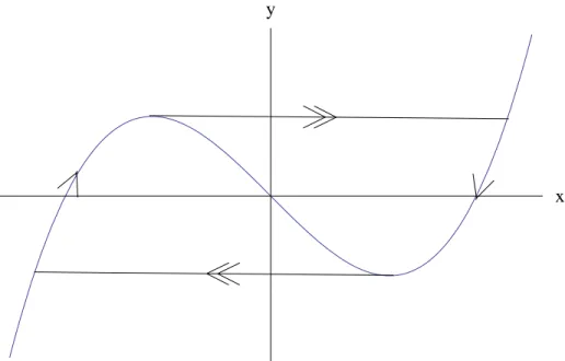
Of course, much of the scientifically interesting behavior in a fast/slow system occurs where GSP theory breaks down, and this is the case in a relaxation oscillation. In the terminology of the previous section, a relaxation oscillation can be constructed from a singular periodic orbit—that is a periodic orbit in the singular limit that consists of trajectories from both the layer problem and the reduced problem. An example in the case where n = m = 1 is depicted in Figure 1.4. The relaxation behavior is provided by a trajectory of the layer problem equilibrating to an attracting branch ofM0. The slow loss of stability occurs as the dynamics of the reduced problem

send trajectories toward an extremum of the critical manifold.

(22)

x y

Figure 1.4. Relaxation oscillation. Oscillation pictured in the

sin-gular limit with an ‘S’-shaped critical manifold. The outer branches (where the curve is increasing) are stable, the middle branch is unsta-ble. The double arrows indicate fast dynamics of the layer problem (relaxation behavior). The single arrows represent slow dynamics of the reduced problem.

is that for all p∈ F,

det

∂f ∂x

p

= 0.

Geometrically, a fold is a set where the critical manifold is tangent to trajectories of the layer problem. Therefore, along the fold, the fast and slow dynamics are tangent. Since the critical manifold cannot be written as{x=h(y)}at the fold, it is a singular set of the slow dynamics. The most common types of fold points are called regular fold points. At a regular fold point, the slow dynamics point toward the fold on both sides or away from the fold on both sides, so the fold point is an essential singularity [33]. A system containing regular fold points where the slow dynamics are directed toward can produce relaxation oscillations since trajectories will reach the sets where metastable states become unstable [34, 63].

In planar systems, there is a special type of fold point called a canard point. A

(23)

occurs when the slow nullcline intersects the critical manifold at the fold. When this happens, the slow dynamics point toward the fold on one side and away from the fold on the other. Because of this, a canard point is a removable singularity of the slow dynamics, and trajectories of the reduced problem may cross the fold from the stable branch of M0 to the unstable branch (or vice versa) [33]. Such a trajectory is called

a singular canard, and it perturbs to canard solutions for >0.

‘Canard’ is a French word with two meanings. The literal translation in Eng-lish is ‘duck,’ however canard can also mean ‘hoax’ or ‘deception.’ Somehow, both translations are appropriate when discussing canards in the mathematical sense. One definition of a canard solution—sometimes called the maximal canard—is a trajec-tory that lies in the intersection of a repelling slow manifold and an attracting slow manifold [33, 34]. A more inclusive definition of a canard solution is a trajectory that remains near a repelling slow manifold for O(1) time. More precisely, the ratio of time spent near repelling slow manifolds to time spent near attracting slow mani-folds isO(1). The existence of a canard solution can lead to a phenomenon known as

canard explosion, whereby a system undergoes a rapid transition from a small limit cycle to relaxation oscillations through a series of canard cycles [3, 18, 19].

The singular canard cycles, built by a combination of pieces ofM0 and transitions

between different branches ofM0, often look like cartoon ducks (see Figure 2.3d), as in

the case of the Van der Pol system. This is the reason the French mathematicians, who first discovered canard cycles, decided to call them ‘canards.’ In planar systems, the canard explosion phenomenon occurs in an exponentially small range of parameters, making canard cycles hard to detect. Because of this difficulty, canard trajectories were misunderstood for a long time. Additionally, it is extremely difficult, if not impossible, to verify their existence in physical experiments.

(24)

expansions [19]. More recently, the popular mechanism for analyzing canards has been a combination of blow-up and dynamical systems techniques. This idea was introduced by Dumortier and Roussarie [18] and generalized by Krupa and Szmolyan [33, 34].

The popularity of the blow-up technique is largely due to the fact that it gener-alizes readily to higher-dimensional systems [62]. In higher dimensions, the analog of a canard point is a folded equilibrium. A folded equilibrium is not the projection of an equilibrium solution of (1.1) onto M0, but rather results from desingularizing

the slow dynamics so that they are defined along the fold F. Certain types of folded equilibria, namely folded nodes, folded saddles, and folded saddle-nodes, result in singular canard orbits [14, 35, 62, 67]. In planar systems, the singular canard may only exist for one particular parameter value, so the effect of a singular canard is hardly seen away from the singular limit. In higher dimensions, a folded equilibrium may produce more than one singular canard orbit, and these orbits exist for a much larger parameter range. Because of this, canard phenomena (such as mixed-mode oscillations) are much more robust in higher dimensions.

This realization cast canards in a new light, spurring the increase of interest in canards over the last decade. Once canards were viewed as somehow being artificial— nuisances that would disappear under small perturbations. Now, canards are under-stood as a possible mechanism for producing more complicated behavior such as mixed-mode oscillations [4, 14]. Indeed, canard trajectories through a folded node are essential to the analysis of the model for glacial-interglacial cycles in Chapter 4— to our knowledge this is the first application of the theory of mixed-mode oscillations to a climate model.

(25)

canards in smooth systems and what are calledquasi-canardsin piecewise-linear sys-tems. First, in the smooth case the explosion phase does not begin immediately upon bifurcation as it does is in the piecewise-linear case. Second, during the explosion, the amplitudes of the periodic orbits in smooth systems grow exponentially, compared to the linear, albeit rapid, growth in the piecewise-linear case. Finally, the shape of the periodic quasi-canard orbits does not change during the explosion. in the smooth canard explosion, the maximal canard causes the periodic orbits to develop an in-flection point. This is due to the existence of a strongly repelling slow manifold, an existence that depends on the nonlinearity of the vector field. The focus of Chapter 2 is on canard phenomena in a piecewise-smooth, planar, fast/slow system that is non-linear. As in the case of smooth systems, a bifurcation occurs as the slow nullcline passes through the extremum of the critical manifold. Conditions are found under which such canard cycles are created from this bifurcation, and in nonlinear piecewise-smooth systems, the canard trajectories resemble piecewise-smooth canards much more than quasi-canards. If these conditions are not met, the system will bifurcate from having a stable equilibrium to having a relaxation oscillation. This transition happens in-stantaneously, forgoing the canard explosion. This behavior, called super-explosion, was first discovered by Desroches et al. in piecewise-linear systems in [15]. A key development of this thesis is demonstrating super-explosion behavior in nonlinear piecewise-smooth systems as well as the possibility of a subcritical super-explosion (where the relaxation oscillation appears before the bifurcation).

(26)

CHAPTER 2

Canard-like Phenomena in Piecewise-Smooth Planar Systems

2.1. Introduction

(27)

The generic nonsmooth, continuous dynamical system can be written as

(2.1) z˙ =

  

FL(z) on{h(z)≤0} FR(z) on{h(z)≥0} where z ∈_Rk _{and there exists an} _n _{such that}

dn_F L dzn

{h(z)=0}

6= d n_F R dzn

{h(z)=0}

.

The co-dimension one set of discontinuities of the nth derivative (i.e., {h(z) = 0}) is called the splitting manifold. We will consider the specific case of planar fast/slow systems where n = 1 and k = 2. In particular, we consider a nonlinear, piecewise-smooth Li´enard system:

(2.2) x˙ =−y+F(x)

˙

y=(x−λ) where

F(x) =   

g(x) x≤0 h(x) x≥0

with g, h∈Cr_{, r}_≥_1, _{g(0) =}_{h(0) = 0,} _g0₍₀₎_<_{0 and} _h0₍₀₎ _>_{0, and we assume that}

h has a maximum atxM >0. The critical manifold

N0 ={y=F(x)}

(28)

-0.5 0.5 1.0

-0.5 0.5 1.0 1.5

Figure 2.1. Example of a ‘2’ shaped critical manifold.

Nonsmooth systems are interesting in two ways: (1) the similarities they share with smooth systems or (2) the ways they differ from smooth systems. This paper addresses both of those issues with regard to systems of the form (2.2). First, we find conditions under which (2.2) exhibits canard phenomena similar to its smooth counterpart. Second, we describe the dynamics when those conditions are not met.

(29)

piecewise-smooth case as well, however our more general setting allows us to demon-strate a sub-critical super-explosion—the simultaneous existence of a stable equilib-rium and a stable relaxation oscillation.

The method of proof employs ashadow system, or smooth system that agrees with (2.2) on one side of the splitting line. In most cases we will use

(2.3) x˙ =−y+h(x)

˙

y=(x−λ)

as our shadow system. For x >0, the systems (2.2) and (2.3) agree. It is often useful to consider a trajectory with initial conditions in the right half-plane, following the flow until the trajectory hits the splitting line {x = 0}. At this point, the vector fields no longer coincide, so the trajectory will behave differently in (2.2) than it will in (2.3). We will compare the different behavior for x < 0, utilizing what is known about canard cycles in smooth systems.

In Section 2.2 we provide the relevant background material required to prove the main results. In Section 2.3 we state and prove the main results about the existence or lack of canard cycles in nonsmooth systems. Finally, we conclude with a discussion in Section 2.4.

2.2. Background

In this section we provide the necessary background material that we will use to prove the results in Section 3.

(30)

x y

(a) λ= 0

x y

(b) λ >0

Figure 2.2. Fast and slow dynamics leading to canard explosion in

the smooth case.

Consider a one-parameter family of singularly perturbed systems in the form

(2.4) x

0 ₌ _{f(x, y, λ, )}

y0 = g(x, y, λ, )

x∈_R y∈_R 0< 1,

where f, g are Ck function with k ≥ 3 and ˙ = d/dt. For the system to undergo a canard explosion, (2.4) must satisfy a series of assumptions.

(A1) The critical manifold, S = {f(x, y, λ,0) = 0} is ‘S’-shaped. That is, it can be written in the form y = φ(x), where φ has precisely two critical points: a non-degenerate local maximum, and a non-degenerate local minimum. Without loss of generality, we assume that the minimum occurs at the origin and the maximum occurs for some x = xM > 0. Then, the critical manifold can be broken into three pieces, Sl, Sm, and Sr—left, middle, and right, respectively—separated by the local extrema of φ. These three pieces are:

Sl ={(x, φ(x)) :x <0} Sm ={(x, φ(x)) : 0 < x < xM}

(31)

(A2) In the layer problem, the outer branches Sl and Sr are attracting, and the middle branch Sm is repelling. That is,

∂f ∂x

Sl,r

<0, and ∂f

∂x

Sm

>0.

(A3) For some value λ = λ0 one of the folds is a non-degenerate canard point.

Without loss of generality, we assume this happens for λ0 = 0 and for the fold point

at the origin (i.e. the fold connecting Sl _and _Sm_).

Similar to (A2), the assumptions (A1) and (A3) can also be expressed in terms of partial derivatives. The condition that (0,0) is a fold point as well as a singularity when λ= 0 gives us

f(0,0,0,0) = 0, ∂f

∂x(0,0,0,0) = 0, g(0,0,0,0) = 0, along with the non-degeneracy assumptions

∂2_f

∂x2(0,0,0,0)6= 0,

∂f

∂y(0,0,0,0)6= 0.

Also, for the canard point to be non-degenerate we get the conditions ∂g

∂x(0,0,0,0)6= 0, ∂g

∂λ(0,0,0,0)6= 0.

Finally, there is one last assumption required for the canard explosion theorems. (A4) When λ = 0, the dynamics of the reduced problem have ˙x < 0 on Sr _and ˙

x >0 on Sl_{∪ {0} ∪}_Sm_.

The flow in the reduced problem is given by the equation

(2.5) x˙ = g(x, φ(x), λ,0)

φ0_(x) .

(32)

x y

(a) Singular canard cycle Γ(s), s ∈

(0, yM).

x y

(b) Singular canard cycle Γ(s),s=yM.

x y

(c) Singular canard cycle Γ(s), s ∈

(yM,2yM).

(d) A duck!

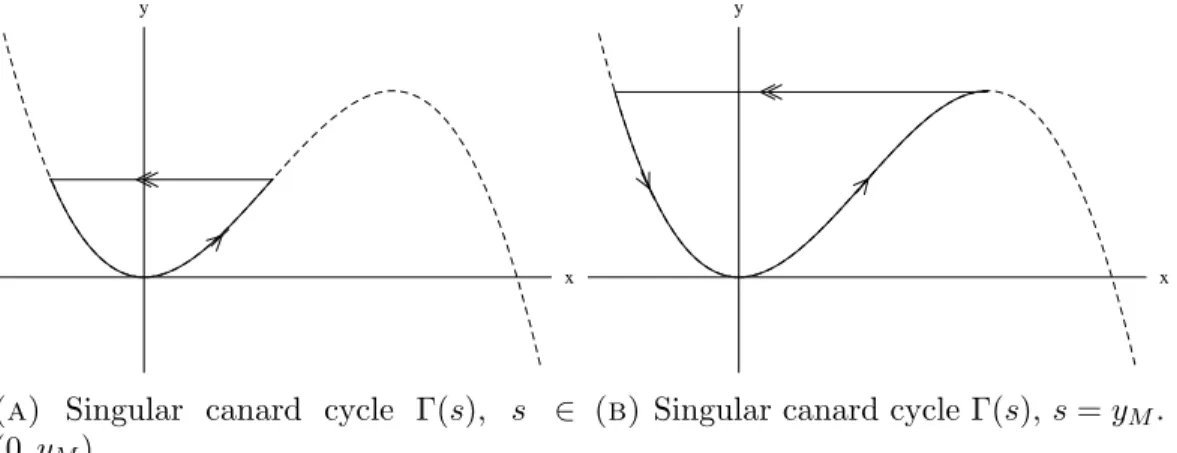
Figure 2.3. Examples of the three types of singular canard cycles: (a)

canard without head, (b) maximal canard, and (c) canard with head.

2.2a. Directly calculating eigenvalues of the Jacobian shows that λ = 0 is precisely when (2.4) undergoes a Hopf bifurcation. When λ = 0, the slow nullcline passes through fold, creating the canard point. In [34], Krupa and Szmolyan show that for some λ > 0 (as in Figure 2.2b) the system (2.4) exhibits relaxation oscillations. The canard explosion is the rapid transition from the small periodic orbits created through the Hopf bifurcation to the large relaxation oscillation. This is shown through a family of singular periodic orbits Γ(s), which we now describe.

(33)

xm(yM) =xM =xr(yM). We can now define Γ(s) piecewise fors ∈[0,2yM]. First,

Γ(s) ={(x, φ(x)) :x∈[xl(s), xm(s)]} ∪ {(x, s) :x∈[xl(s), xm(s)]}, for s∈[0, yM].

This is a singular orbit like the one in Figure 2.3a (for s 6=yM), often referred to as a “canard without head.” Next,

Γ(s) ={(x, φ(x)) :x∈[xl(yM), xm(2yM −s)]}

∪ {(x,2yM −s) :x∈[xm(2yM −s), xr(2yM −s)]} ∪ {(x, φ(x)) :x∈[xM, xr(2yM −s)]}

∪ {(x, yM) :x∈[xl(yM), xM]} for s∈[yM,2yM].

In the second case (for s 6=yM), Γ(s) traces out an orbit like the one in Figure 2.3c, beginning at the left-most point and following the arrows in the directions indicated in the figure. Orbits of this type are called “canards with head.” When s =yM, we get the maximal canard as shown in Figure 2.3b.

The idea behind the canard explosion theorems is explained by Krupa and Sz-molyan [34] as being

“to obtain a family Γ(s, ) of canard cycles existing for corresponding parameter values λ = λ(s, ) as a perturbation of the degenerate family Γ(s), λ = 0 which exists for = 0. As s sweeps through a suitable interval of the family of canard cycles Γ(s, ) connects the Hopf bifurcation to relaxation oscillations and canard explosion takes place.”

Near the non-degenerate canard point, there is a canonical form for (2.4):

(2.6) x

0 ₌_−yh

1(x, y, λ, ) +x2h2(x, y, λ, ) +h3(x, y, λ, )

(34)

where

h3(x, y, λ, ) =O(x, y, λ, )

hj(x, y, λ, ) = 1 +O(x, y, λ, ), j = 1,2,4,5. Define the constants

a1 =

∂h3

∂x (0,0,0,0), a2 = ∂h1

∂x (0,0,0,0), a3 = ∂h2

∂x (0,0,0,0), a4 =

∂h4

∂x (0,0,0,0), a5 =h6(0,0,0,0), and

(2.7) A=−a2+ 3a3−2a4−2a5.

Finally, we define the function R(s), which is called the “way in-way out” function in [3]. Similar to Γ(s), we define R(s) for s ∈[0,2yM], but differently for s > yM or s < yM. We have

R(s) =

Z xm(s)

xl(s)

∂f

∂x(x, φ(x),0,0)

φ0(x)

g(x, φ(x),0,0)dx for s ∈[0, yM], and

R(s) =

Z xm(2yM−s)

xl(s)

∂f

∂x(x, φ(x),0,0)

φ0(x)

g(x, φ(x),0,0)dx +

Z xM

xr(2yM−s)

∂f

∂x(x, φ(x),0,0)

φ0(x)

g(x, φ(x),0,0)dx for s∈[yM,2yM]. We are now ready to state the theorems of canard explosion. The first theorem describes the Hopf bifurcation, out of which the small canard cycles are born [34].

Theorem 2.2.1. Suppose (A1)-(A4) hold. Then there exist 0 > 0 and λ0 > such that for each 0 < < 0 and each |λ| < λ0, the system (2.4) has precisely one equilibrium pe which converges to the canard point as(, λ)→0. Moreover, there

exists a curveλH( √

)such thatpe is stable forλ < λH( √

(35)

a Hopf bifurcation as λ passes through λH( √

). The curve λH( √

) has the expansion

λH( √

) = −a1+a5

2 +O(

2_).

The Hopf bifurcation is non-degenerate if A is nonzero. It is supercritical if A < 0

and subcritical if A >0.

The second theorem proves the existence of maximal canards. A maximal canard is a trajectory that connects a stable slow manifold to an unstable slow manifold. This happens precisely when slow manifoldsSl

andSm change their relative position. The existence of the slow manifolds is guaranteed by Fenichel theory, however they are, in general, not unique. In [33] it is demonstrated that the lack of uniqueness does not pose a problem in demonstrating the existence of a unique maximal canard.

Theorem 2.2.2. Suppose that (A1)-(A4) hold. Then there exists a smooth func-tionλc(

√

)such that a solution starting inSl

connects toSm if and only λ=λc( √

). The function λc has the expansion

λc( √

) = −

a1+a5

2 +

1 8A

+O(3/2_).

(36)

Theorem2.2.3. Fix0 sufficiently small and v ∈(0,1). Assume (A1)-(A4) hold, and assume A <0. For ∈(0, 0) there exists a family of periodic orbits

s→(λ(s,√),Γ(s,√)), s∈(0,2yM)

which is Ck _{smooth in} _(s,√₎_{, and such that}

(i) for s ∈ (0, v) the orbit Γ(s,√) is attracting and uniformly O(v₎ _{close to the}

canard point and λ(s,√) is strictly increasing in s, (ii) for s∈(2yM−v,2yM)the orbitΓ(s,

√

)is a relaxation oscillation andλ(s,√)

is strictly increasing in s, (iii) if s∈[v_,_2y

M −v], then |λ(s, √

)−λc( √

)| ≤e−1/1−v

;

(iv) as →0, the family Γ(s,√) converges uniformly in Hausdorff distance toΓ(s); (v) any periodic orbit passing sufficiently close to the critical manifoldS is a member

of the family Γ(s,√) or a relaxation oscillation.

Theorem 2.2.3 guarantees a canard explosion takes place in the situation of a sub-critical Hopf bifurcation, so we can define the functions λs(

√

) = λ(v,√) and λr(

√

) =λ(2yM−v, √

),which mark the beginning and end of the canard explosion. The subscripts s and r stand for small and relaxation cycles, respectively. The stability of the orbits and the monotonicity of the λj(s,

√

) depends on R(s). For more information and figures of these curves, we direct the reader to Krupa and Szmolyan’s work [34].

Theorem 2.2.4. If the assumptions of Theorem 2.2.3 hold and R(s) <0 for all

s ∈(0, yM], then all canard cycles are stable and the functions λj (where j= H, s, c,

or r) are monotonic in s.

(37)

Theorem2.2.5. Fix0 sufficiently small and v ∈(0,1). Assume (A1)-(A4) hold, and assume A >0. For ∈(0, 0) there exists a family of periodic orbits

s→(λ(s,√),Γ(s,√)), s∈(0,2yM)

which is Ck _{smooth in} _(s,√₎_{, and such that}

(i) for s ∈ (0, v₎ _{the orbit} _Γ(s,√₎ _{is repelling and uniformly} _O(v₎ _{close to the}

canard point and λ(s,√) is strictly increasing in s, (ii) for s∈(2yM−v,2yM)the orbitΓ(s,

√

)is a relaxation oscillation andλ(s,√)

is strictly increasing in s, (iii) if s∈[v_,_2y

M −v], then |λ(s, √

)−λc( √

)| ≤e−1/1−v_;

(iv) as →0, the family Γ(s,√) converges uniformly in Hausdorff distance toΓ(s); (v) any periodic orbit passing sufficiently close to the critical manifoldS is a member

of the family Γ(s,√) or a relaxation oscillation.

The curves λs and λr are defined the same in the case of the subcritical Hopf bifurcation, however, the orientation of all of theλj curves is reversed [34].

2.2.2. Quasi-canards in Piecewise Linear Systems. In [15], Desroches et al.

consider a piecewise-linear fast/slow Li´enard system of the form:

(2.8) x

0 ₌_−y₊_f_(x)

y0 =(x−λ), where

f(x) =         

−x, x <0, kx, 0≤x≤2, −x+ 2(k+ 1), x >2,

(38)

the ‘S’-shape of the manifold, we will think of it as representing the smoothness. In a similar manner, we define

Ll ={(x, f(x)) :x <0} Lm ={(x, f(x)) : 0< x < 2}

Lr ={(x, f(x)) :x >2},

where the L stands for linear. The system will always have an equilibrium point at (λ, f(λ)). It is easy to check that for λ < 0 (and λ > 2) the equilibrium is stable. When 0 < λ < 2, the equilibrium is unstable and Poincar´e-Bendixson guarantees the existence of a stable periodic orbit. This is especially easy to see in the singular limit, and is not significantly more difficult for >0. Thus, whenλ= 0 (and λ= 2), there must be a bifurcation by the which the periodic orbits are created asλincreases (resp. decreases) through the bifurcation value. The main result of [15] characterizes this bifurcation.

Since the system is piecewise-linear, f0(x) is constant in each linear zone. That is,

f0(x) =         

−1, x < 0, k, 0≤x≤2, −1, x > 2.

Therefore, for fixed , the eigenvalues of the system are also constant in each linear zone. A quick computation shows that the eigenvalues for an equilibrium onLl _or_Lr are

λ±=

−1±√1−4

2 ,

so for ≤ 1/4, the critical points will be nodes. Otherwise they will be stable foci. For an equilibrium onLm_{, the eigenvalues are}

λ± =

k±√k2₋₄

(39)

and the type of equilibrium (unstable focus or unstable node) is determined by the sign of k2−4.

Theorem 2.2.6. In the system (2.8), for 0< ≤ 1₄ andk > 0fixed, the following statements hold:

(i) For λ < 0 the equilibrium is globally asymptotically stable and, therefore, it is the global attractor of the system.

(ii) For λ= 0, the equilibrium point is always the global attractor of the system; it is globally asymptotically stable whenk2₋_{4 <}₀_{(the focus case), but it is unstable} fork2−4 >0(the node case). The instability of this latter case comes from the existence of a bounded continuum of homoclinic orbits to the equilibrium point,

the most external homoclinic orbit defined by the unstable invariant manifold

that coincides for 0≤x≤2 with the straight line

y= k− √

k2₋₄

2 x

and eventually coming back to the equilibrium, approaching it tangentially to the

straight line

y=−1 + √

1−4

2 x

.

(iii) For 0 < λ < 2, the equilibrium point is unstable and surrounded by a unique stable limit cycle.

(a) When k2−4≥0 (the node case), the limit cycle always has points in each of the three linearity zones.

(40)

two positive constants λG(k, ) and m(k, ) such that

α(λ) =m(k, )·λ

for 0 < λ < λG. Furthermore, the length of the linear range λG and the linear

growth rate m satisfy

lim k→2√−

λG = 0 and lim k→2√−

m = +∞.

As the theorem states, the two possibilities for the bifurcation are (iii)(a) a transi-tion from a stable node to an unstable node or (iii)(b) a transitransi-tion from a stable node to an unstable focus. In the first case, the system transitions from having a globally attracting equilibrium to relaxation oscillations without undergoing anything resem-bling the canard explosion described in the previous subsection. Desrocheset al. [15] coin the term super-explosionto describe this instantaneous jump. In the latter case, λG corresponds to λc in that it is the value of λ for which the stable periodic orbit intersects the local maximum of the critical manifold {y=f(x)}. In contrast to the smooth canard explosion (for the supercritical Hopf case), the “explosion” phase in the piecewise-linear case occurs immediately upon bifurcation and stops at λG (see Figure 2.4b). The subscript G denotes that this occurs precisely at the value of λ for which a grazing bifurcation occurs—this is, the value of λ for which the stable periodic orbit is tangent to the splitting line x= 2.

(41)

−2 −1 0 1 2 3 −0.5 0 0.5 1 1.5 X Y

(a) Canard cycles in the piecewise linear

system (2.8) with k= 0.4,= 0.2.

−0.5 0 0.5 1

−0.5 0 0.5 1 1.5 2 2.5 3 3.5 λ Amplitude

(b) Growth of amplitudes of periodic

or-bits asλincreases.

Figure 2.4. Depiction of the quasi-canard explosion.

never develop heads—the singular canard with head in smooth systems is depicted in Figure 2.3c. The inclusion of a fourth linear zone, one with a strongly repelling slow manifold betweenLm_and _Lr_{, is enough to produce canards with heads [47]. Another} important distinction, which was not discussed in [15], is the possibility of subcritical “Hopf-like” bifurcations. As we will see, it is possible to have a quasi-canard cycle or relaxation oscillation appear before the equilibrium loses stability, however this relies on the slope of Ll _{being sufficiently small.}

2.2.3. Nonsmooth Hopf Bifurcations. Finally, we introduce the last big piece of the puzzle, a criterion for determining when a nonsmooth Hopf bifurcation is sub-or super-critical. Unlike the complicated criterion fsub-or smooth Hopf bifurcations that relies on third order mixed partials [25], Simpson and Meiss showed that the criterion for nonsmooth Hopf bifurcations is astoundingly simple [60].

The main result from [60] considers a planar, piecewise-Ck_{, continuous system of} ODEs with k ≥1 of the form

(2.9) z˙ =

  

FL(x, y;λ), x≤0 FR(x, y;λ), x≥0

,

(42)

Theorem 2.2.7. Suppose that the vector field (2.9) is continuous and piecewise

Ck, k ≥ 1, in (x, y, λ) and has an equilibrium that transversely crosses a one-dimensional switching manifold when λ = 0 at a point z∗ where the manifold is Ck_.

Suppose further that as λ % 0 the eigenvalues of the equilibrium approach µu ±iωu

and as λ &0 they approach −µs±iωs, where µu, µs, ωu, ωs>0. Define

Λ = µu ωu

− µs ωs .

Then if Λ<0 there exists an >0 such that for all 0< λ < there is an attracting periodic orbit whose radius is O(λ) away from z∗, and for − < λ < 0 there are no periodic orbits near z∗.

If, on the other hand, Λ >0, there exists an > 0 such that for all − < λ < 0

there is repelling periodic orbit whose radius is O(λ) away from z∗, and for all 0 < λ < there are no periodic orbits near z∗.

2.3. Main Results

As we state and prove our main results, we will consider systems of the form

(2.10) x˙ =−y+F(x)

˙

y=(x−λ) where

F(x) =   

g(x) x≤0 h(x) x≥0 and the following assumptions hold

(I) g, h∈Ck_{, k}_≥_1, (II) g(0) =h(0) = 0, (III) g0(0)<0,

(IV) h0(0)>0,

(43)

The critical manifold

N0 ={y=F(x)}

is ‘S’-shaped with a smooth fold at xM and a corner along the splitting line x = 0. As for the smooth and piecewise linear cases, we denote

Nl={(x, F(x)) :x <0}={(x, g(x)) :x <0}

Nm ={(x, F(x)) : 0< x < xM}={(x, h(x)) : 0< x < xM} Nr ={(x, F(x)) :x > xM}={(x, h(x)) :x > xM}.

We will assume that h(x) can be extended into the region where x < 0 and define the shadow system to be

(2.11) x˙ =−y+h(x)

˙

y=(x−λ).

Since there are two distinct types of bifurcation that can lead to the formation of periodic orbits—one at the smooth fold and one at the corner—we will consider each of those cases separately. In both cases, we will consider the relative distance from the origin of trajectories in the nonsmooth system (2.10) and shadow system (2.11) that enter the left half-plane x < 0 at the same point (0, y∗). The following lemma

describes the relationship of these trajectories.

Lemma 2.3.1. Consider the trajectoryγn(t) = (xn(t), yn(t)) of (2.10) that crosses

the y-axis entering the left half-plane x < 0 at γn(0) = (0, yc). Also consider the

analogous trajectory γs of the shadow system (2.11). The condition on the slopes of g, h at 0 in (2.10) guarantee that g(x) > h(x) for some range of x’s where x < 0. Assume g(x) > h(x) arbitrarily far into the left half-plane. Then, the distance from the origin of γn is bounded by that of γs.

Proof. Define

R(x, y) = x

2₊_y2

(44)

R will evolve differently in the nonsmooth and shadow systems when x < 0, so we denote ˙Rn(x, y) and ˙Rs(x, y) as the time derivative ofRin the nonsmooth and shadow systems, respectively. Then we have

˙

Rn(x, y) = x(g(x)−y) +y(x−λ) ˙

Rs(x, y) = x(h(x)−y) +y(x−λ).

Therefore, at a given point (x, y) wherex≤0, we have

˙

Rn(x, y)−R˙s(x, y) = x[g(x)−h(x)]≤0,

since g(x) ≥ h(x), where equality only holds if x = 0. Thus, γn can never cross γs moving away from the origin for x < 0 (i.e., in the left half-plane the vector field of (2.10) points “inward” on the trajectory γs). Since γn and γs coincide at (0, yc), it suffices to show that R(γn(δt)) < R(γs(δt)) for δt > 0 sufficiently small. Since the vector fields of (2.10) and (2.11) coincide on the y-axis, we must use second order terms:

 

xn(δt) yn(δt)

 =

 

0 + ˙xnδt+ ¨xnδt2 yc+ ˙ynδt+ ¨ynδt2

  



xs(δt) ys(δt)

 =

 

0 + ˙xsδt+ ¨xsδt2 yc+ ˙ysδt+ ¨ysδt2

 .

We have already seen that (xs(t), ys(t)) and (xn(t), yn(t)) agree for the 0thand 1st order terms. Therefore, the important terms are

¨

xn = −y˙n+g0(0) ˙xn =λ−g0(0)yc ¨

xs = −y˙s+h0(0) ˙xs =λ−h0(0)yc and

¨

yn = x˙n =−yc ¨

(45)

Figure 2.5. Relative slopes of vectors as discussed in the proof of

Lemma 2.3.1.

Both vector fields point left ( ˙x <0 ) if and only ify >0, soycmust be positive. Since ¨

y is the same in both systems, we look at the ¨x terms. Since −g0₍₀₎ _> ₀ _>_−h0_(0),

the smooth trajectory of the shadow system moves further left than the nonsmooth trajectory for the same vertical change as in Figure 2.5. This shows that the trajectory of the nonsmooth system enters the left half-plane immediately below (i.e., nearer to the origin than) the trajectory of the shadow system. Onceγn is nearer to the origin

than γs, it is bounded by γs, proving the result.

Corollary 2.3.2. Consider the trajectory γn(t) = (xn(t), yn(t)) of (2.10) that

crosses the y-axis entering the left half-plane x < 0 at γn(0) = (0, yc). Also consider

the analogous trajectory γS of the system

(2.12) x˙ =−y+ ˜F(x)

˙

y=(x−λ)

where

˜ F(x) =

  

˜

g(x) x≤0 h(x) x≥0

and g˜0(0) > g0(0). Then, the radial distance from the origin of γn is bounded by that

of γS.

Proof. The proof of Lemma 2.3.1 only used that g0(0) < h0(0), not requiring

(46)

2.3.1. Canards at the smooth fold.

Theorem 2.3.3. Fix 0< 1. In system (2.10), assume (I)−(V) hold. Then there is a Hopf bifurcation when λ = xM. If the Hopf bifurcation is non-degenerate,

then it will produce canard cycles.

Proof. Direct calculation shows that (2.10) undergoes a Hopf bifurcation at

λ =xM. The criticality of the Hopf bifurcation is determined as usual [25], since it is a smooth Hopf bifurcation. Assume the criticality parameter is nonzero (i.e. the bifurcation is non-degenerate). Let Γn

(λ) denote the family of stable periodic orbits in the nonsmooth system, and Γs(λ) denote the family for the smooth (shadow) system. For someλG(), the system undergoes a grazing bifurcation where the stable periodic orbit is tangent to the splitting linex= 0 (which necessarily happens at (0,0) since it happens on thex nullcline). If Γs(λ)⊂ {x >0} (which happens for allλG< λ < xM in the supercritical case), then Γs_{= Γ}n_.

Beyond the grazing bifurcation (i.e. for λ < λG), Γs must cross the y-axis trans-versely. Letyc>0 be they-coordinate of the crossing into the left half-plane, and let yd < 0 be the y-coordinate where Γs re-enters the right half-plane. Define γn to be the trajectory of (2.10) through the point (0, yd). Without loss of generality, assume γn(0) = (0, yd). Then there exists a time tc > 0 so that γn(tc) = (0, yc) and for all t∈[0, tc],γn coincides with Γs. By Lemma 2.3.1 for all t > tc,γn must be contained in the interior of Γs. In particular, there exists a pair (td, yd∗) withtd> tcandyd∗ > yd, such that γn(td) = (0, yd∗). Let V be the set enclosed by the closed curve

∂V ={γn(t) : 0 ≤t ≤td} ∪ {(0, y) :yd∗ ≤y≤yc}

The vector field of (2.10) is either tangent to or pointing inward on the ∂V, so Poincar´e-Bendixson guarantees the existence of a stable periodic orbit on the interior

(47)

-2.0 -1.5 -1.0 -0.5 0.5 1.0 1.5 x

-2.0

-1.5

-1.0

-0.5 0.5 1.0

y

Figure 2.6. The setV for a givenλ. The dashed curve is the periodic

orbit of the shadow system. The bold curve is the trajectory in the nonsmooth system. V is the positively invariant set enclosed by the bold curve and the y-axis.

There is a simple corollary to Theorem 2.3.3.

Corollary 2.3.4. Assume the shadow system (2.11)satisfies assumptions (A1)-(A4). The parameter A (as defined in (2.7)) determines the criticality of the Hopf bifurcation according to Theorem 2.2.1. Furthermore, the Γn_(λ) _{are bounded by the}

stable canard orbits.

Given that canard explosion happens in smooth systems, the result should not be surprising. Perhaps more surprising is the possibility of having canard cycles arise as a result of a nonsmooth, Hopf-like bifurcation at λ = 0, explained in the following theorem. Figure 2.7 depicts the canard explosion at a smooth fold and a corner as a result of supercritical Hopf bifurcations in (2.10).

(48)

−2 −1 0 1 2 3 −2 −1 0 1 2 3 4 X Y

(a) Nonsmooth canard cycles in the

supercritical case. The black orbits depict cycles before the explosion at both the smooth fold and the corner. The blue orbit is a post-explosion ca-nard with head at the corner. The red orbit is a post-explosion canard with head at the smooth fold.

−1 −0.5 0 0.5 1 1.5 2

0 0.5 1 1.5 2 2.5 3 λ Amplitude

(b) Amplitudes of nonsmooth

ca-nard cycles in the supercritical case, showing the explosion at the corner (on the left) and smooth fold (on the right).

0.0120 0.0125 0.013 0.0135 0.014 0.0145 0.015

0.5 1 1.5 2 2.5 3 λ Amplitude

(c) A closer look at the explosion at

the corner.

1.5 1.55 1.6 1.65 1.7

0 0.5 1 1.5 2 2.5 3 λ Amplitude

(d) A closer look at the explosion at

the fold.

Figure 2.7. Images characterizing a nonsmooth canard explosion for

= 0.2. The bifurcations are supercritical at both the fold and the corner.

Theorem 2.3.5. In system (2.10), assume (I)−(V) hold. The system undergoes a bifurcation for λ= 0 by which a stable periodic orbit Γn_(λ) _{exists for} ₀ _{< λ < x}

M.

There exists an0 such that for all0< < 0 the nature of the bifurcation is described by the following:

(i) If 0< h0(0) <2√, then canard cycles Γn(λ)are born of a Hopf-like bifurcation as λ increases through 0. The bifurcation is subcritical if |g0_(0)| _< _|h0_(0)| _and

(49)

(ii) If h0(0) > 2√, the bifurcation at λ = 0 is a super-explosion. The system has a stable periodic orbit Γn(λ), and Γn(λ) is a relaxation oscillation. If |g0_{(0)| ≥}

2√, the bifurcation is supercritical in that no periodic orbits appear for λ < 0. However, if |g0_(0)|_<₂√ _{the bifurcation is subcritical, in that a stable periodic}

and stable critical point coexist simultaneously for some λ <0.

Proof. The system always has a unique critical pointpλ = (λ, F(λ)), and direct computation of the corresponding eigenvalues shows that

(2.13) µ±(λ) =

          

g0(λ)±p[g0_(λ)]2₋₄

2 , λ <0 h0(λ)±p[h0_(λ)]2₋₄

2 , λ >0.

For 0 < λ < xM we have h0(λ) > 0, so both eigenvalues have Re(µ±) > 0 and

the critical point pλ is unstable. To demonstrate the existence a stable periodic orbit Γn(λ), it suffices to show that there is a positively invariant set containing pλ. Consider the set W as shown in Figure 2.8. The boundary ∂W is composed of six line segments lj forj = 1, 2, . . .6. Choose any point (ˆx,0) with ˆx <0.

l1 ={(x, y) :y=m1(x−x), mˆ 1 <0 is O(1), xˆ≤x≤λ}

l2 ={(x, y1) :y1 =m1(λ−x), λˆ ≤x≤x2 = (h−1(y1) + 1)}

l3 ={(x2, y) :y1 < y < y3 =h(xM)} l4 =

(x, y) :y=m4(x−x2) +y3 wherem4 >

g(ˆx)−y3

λ−x2

is O(1)

l5 ={(x, y5) :y5 =m4(λ−x2) +y3, x < x < λ}ˆ

l6 ={(ˆx, y) : 0 < y < y5}

(50)

1

2

6

5

4

3

Figure 2.8. An example of a setW which is positively invariant. The

numbers indicate the 6 line segments li forming the boundary ∂W.

Γn(λ) for 0< λ < xM. The Γn created through the bifurcation at λ= 0 will differ in amplitude depending on h0(0).

First, we consider the case where 0 < h0(0) < 2√. If |g0_(0)| _< ₂√ _{as well, the}

bifurcation atλ = 0 is the nonsmooth Hopf bifurcation discussed in Section 2.3, and Theorem 2.9 applies. In correspondence with Theorem 2.9, we have

µu =h0(0) µs=|g0(0)| ωu =

p

(4−[h0_(0)]2₎

ωs= p

(4−[g0_(0)]2_),

and

Λ = µu ωu

(51)

Thus

Λ<0 ⇐⇒ µu ωu

< µs ωs

⇐⇒ h0(0)p[4−g0_(0)]2 _<_|g0_(0)|p₄₋_[h0_(0)]2

⇐⇒ 4[h0(0)]2−[h0(0)]2·[g0(0)]2 <4[g0(0)]2[h0(0)]2·[g0(0)]2 ⇐⇒ [h0(0)]2 <[g0(0)]2.

Therefore, there is a subcritical nonsmooth Hopf bifurcation when h0(0) < |g0_(0)|

and supercritical nonsmooth Hopf bifurcation when h0(0) > |g0_{(0)|. Corollary 2.3.2,}

also guarantees the existence of canard cycles for the case where |g0_(0)|_>₂√_{. The}

bifurcation in that case is a stable node-to-unstable focus. The canard cycles in the system with a node will be contained in the cycles for the system with a nonsmooth Hopf (stable focus-to-unstable focus) bifurcation. This proves assertion (i).

Next, we consider the case whereh0(0) ≥2√.In this case, forλ >0 (but bounded away from xM), the critical point pλ is an unstable node. Let µ2 ≥ µ1 > 0 be the

strong and weak unstable eigenvalues corresponding to pλ. Also, let v1,2 = (x1,2, y1,2)

be the associated eigenvectors. Then fori= 1,2 we have h0(λ)xi−yi =µixi xi =µiyi.

This implies that the slope of the eigenvector

v2 =

µ2

.

Now, µ2 depends on , however µ2 →2h0(λ) as → 0. Thus for sufficiently small,

we can make the slope of v2 as flat as we like. Therefore, there exists an 0 such that

for all 0< < 0, the strong unstable trajectory must enter the region of phase space

(52)

−0.5 0 0.5 1 1.5

−0.2 0 0.2 0.4 0.6 0.8 1 1.2

X

Y

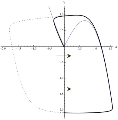
Figure 2.9. The stable orbit of a super-explosion (blue) for = 0.2.

The line x=λ (red) is the slow nullcline. Hereλ= 0.001.

y= 0. Following the trajectory further, it must continue downward to the right until it reaches the y-nullcline x = λ at some point (λ,y) where ˆˆ y < h(λ). Let V be the region enclosed by the trajectory described above and the line segment along x= λ connecting ˆy and h(λ). All trajectories in W that start outside of V are bounded outside ofV (see Figure 2.10a). Therefore Γn_{(λ) must be a relaxation oscillation, and} the bifurcation must be a super-explosion, as depicted in Figure 2.9.

Suppose also that g0(0) ≥ 2√. Then, for λ < 0 the equilibrium pλ is a stable node. It is the global attractor of the system (as in Theorem 2.2.6) since, the strong stable trajectory topλ bounds trajectories above the node in the left half-plane. Since no stable periodic orbits can coexist with pλ, we say the bifurcation is supercritical.

(53)

W

V

-0.5 0.5 1.0

-0.5 0.5 1.0 1.5

(a) The setW \V forλ= 0.014.

V ' W

-1.0 -0.5 0.5 1.0 1.5

-1.5 -1.0 -0.5 0.5 1.0 1.5 2.0

(b) The setW \V0 forλ=−0.05.

Figure 2.10. Positively invariant sets. These sets demonstrate the

existence of attracting periodic orbits for (a) the standard (supercriti-cal) super-explosion and (b) the subcritical super-explosion. W is the region bounded by the six (green) line segments as in Figure 2.8. The sets enclosed by the bold trajectory are (a) V or (b) V0.

(see Figure 2.10b). Therefore, there must be an attracting periodic orbit Γn_{(λ) inside} W \V0. Since an attracting critical point and an attracting periodic orbit coexist simultaneously, we call this a subcritical super-explosion. This proves assertion (ii).

There are two simple corollaries to Theorem 2.3.5.

Corollary 2.3.6. Consider the system with two corners and no smooth folds

(2.14) x˙ =−y+F(x)

˙

y=(x−λ)

where

F(x) =         

g(x) x≤0 h(x) 0≤x≤xM f(x) xM ≤x

with g, h, f ∈ Ck_{, k} _≥₁_, _{g(0) =}_{h(0) = 0}_, _f(x

M) = h(xM) g0(0) <0, h0(x) > 0 for

all 0 < x < xM, and f0(xM) < 0. The system undergoes a bifurcation for λ = 0 by

which a stable periodic orbit Γn_(λ) _{exists for} ₀ _{< λ < x}

(54)

(i) If 0< h0(0) <2√, then canard cycles Γn_(λ)_{are born of a Hopf-like bifurcation}

as λ increases through 0. The bifurcation is subcritical if |g0_(0)| _< _|h0_(0)| _and

supercritical if |g0_(0)|_>_|h0_(0)|.

(ii) If h0(0) > 2√, the bifurcation at λ = 0 is a super-explosion. The system has a stable periodic orbit Γn(λ), and Γn(λ) is a relaxation oscillation. If |g0_{(0)| ≥}

2√, the bifurcation is supercritical in that no periodic orbits appear for λ < 0. However, if |g0_(0)|_<₂√ _{the bifurcation is subcritical, in that a stable periodic}

and stable critical point coexist simultaneously for some λ <0.

Proof. The proof is the same as that of Theorem 2.3.5, only we use (2.10) as

our shadow system.

The second corollary is an immediate application of Lemma 2.3.1.

Corollary 2.3.7. Fix > 0. Assume the shadow system (2.11) satisfies the assumptions (A1)-(A4) for a canard point at (xm, h(xm)) where xm < 0. Then for

fixed λ ∈ (0, xM), Γn(λ) is bounded by the periodic orbit Γs of the shadow system.

Furthermore, if A < 0 and |xm| < λs( √

), then (2.10) will undergo a canard explo-sion.

We have demonstrated that there are two types of nonsmooth bifurcations in which periodic orbits appear before the parameter reaches the bifurcation value. We will show that these are truly subcritical bifurcations. In other words, as the bifurcation parameter moves away from the bifurcation value, the periodic orbits are destroyed.

Proposition 2.3.8. In a system of the form (2.10) for which there exists an

m <0 such that g0(x)≤m <0 for all x <0. Then there exists a K >0 such that if

λ <−K, the system has no periodic orbits.

Proof. The idea of the proof is amounts to using a variation of Dulac’s criterion

[25] for the non-existence of periodic orbits. Define

(55)

so G(x, y) is the vector field. We will need to use the divergence ∇ ·G often, and direct computation shows

∇ ·G=F0(x).

First, ifλ <0, the only critical point lies in the left half-plane. Since any periodic orbit of a planar system must encircle a critical point, there can be no periodic orbits entirely contained the set x≥0.

Secondly, there can be no periodic orbits entirely contained in the left half-plane. We will show this by contradiction. Suppose there is a periodic orbit Γ contained entirely in the left half-plane, and define D to be the region enclosed by Γ. Then

∇ ·G≥m for all x <0.

Therefore,

Z Z D

∇ ·Gdxdy <0. But by the divergence theorem

Z

Γ

(n·F)ds= Z Z

D

∇ ·F dxdy.

However, Γ is a trajectory, so Z

Γ

(n·G)ds = 0, and we have a contradiction.

We will show that there are no periodic orbits that cross x= 0 in a similar way. Suppose there is a periodic orbit that crosses x = 0. Then it must do so twice; let p1 = (0, y1), p2 = (0, y2) with y1(λ) >0> y2(λ) be the points where Γ intersects the

y-axis. Also, define B(λ) = y1(λ)−y2(λ). Note that B(λ) is the maximum vertical

amplitude of the periodic orbit in the region x ≥0. Let k be the maximum slope of h(x) on the interval 0≤x≤xM. Since F0(x)≥0 only the setx∈[0, xM], we know

Z Z

D∩{x≥0}

∇ ·Gdxdy≤ Z Z

R(λ)

(56)

Figure 2.11. Important sets for the proof of Proposition 2.3.8. ∇·G <

0 is negative on the interior of the triangle D∗(λ) (blue). ∇ ·G|_D >0 on a region bounded by the rectangle R(λ) (red).

where R(λ) is the rectangle with B(λ) forming the left side and having width xM. Next, let p0 = (x0, y0) be the point where Γ intersects the fast nullcline y=g(x), for

x0 < λ. Define B1(λ) to be the line segment connecting p0 top1 and B2(λ) to be the

line segment connecting p0 top2. Then B1 and B2 have constant slope (for fixed λ).

Let D∗(λ) be the interior of the triangle enclosed by B(λ), B1(λ), and B2(λ). Then

D∗ must lie entirely inside D. Along B1 near p1, the vector field must point out of

D∗. Since the slopes of the vectors are monotonically decreasing along B1, if Γ were

ever to crossB1 somewhere other than the endpoints, Γ would be trapped inside D∗.

This would contradict that p0 lies on Γ. A similar argument in reverse time shows

that Γ cannot cross B2. Figure 2.11 areas of the sets D∗(λ) and R(λ).

If we let A(λ) be the area of the region D∗(λ), then

A(λ)> |λ| 2 B(λ). Since g0(x)≤m <0, we have

Z Z

D∩{x<0}

∇ ·Gdxdy < Z Z

D∗

∇ ·Gdxdy < mλ 2B(λ). Thus, ifλ <2xM_mk, we can conclude

Z Z D

(57)

Therefore, by the divergence theorem, Γ cannot be a periodic orbit.

2.4. Discussion

In this chapter, we have demonstrated the existence of canard cycles in planar non-smooth fast/slow systems with a piecewise-non-smooth ‘S’-shaped critical manifold, push-ing the theory beyond piecewise linear systems. Through comparison with smooth shadow systems, we have shown that the amplitudes of canard cycles in nonsmooth systems are bounded by the amplitudes of canard cycles in corresponding smooth systems. As we see in Figure 2.7, it is possible for a corner to produce canards with head, and there is a delay between the bifurcation and the explosion phase. This is a contrast to the piecewise linear case, where the quasi-canards are unable to produce the variety with heads, and the explosion phase begins immediately upon bifurcation. In this respect, canards in piecewise smooth systems are more like their cousins in smooth systems. On the other hand, the splitting line is essential for super-explosion. The instantaneous transition from a globally attracting equilibrium point to relax-ation oscillrelax-ations is a product of the nonsmooth nature of the system. One can think of this work as bridging the gap between what is known about canards in smooth systems on one side and piecewise linear systems on the other side.

This work does not put to bed entirely the theory of canards in piecewise-smooth planar systems. We considered specifically the case where the splitting line and slow nullcline were both vertical lines (i.e. orthogonal to the fast direction). It is probably not too difficult to generalize the work of this paper to the more general case where the splitting line and slow nullcline are parallel. Potentially more difficult would be generalizing the work here to a situation where the slow nullcline intersects the splitting line or even is piecewise-smooth itself.

(58)

(59)

CHAPTER 3

Relaxation Oscillations in an Idealized Ocean Circulation

Model

3.1. Introduction

An important aspect of the climate system is the variability in the climate record. An understanding of this variability, specifically with regard to glacial millennial cli-mate change, has remained elusive (see [11]). In different eras of Earth’s history, the variations themselves change in both period and amplitude. It is even possible to have small oscillations superimposed over larger oscillations. Increasingly, scientists are utilizing improved technology to study the climate system through high-powered computer simulations. Large scale oscillations and critical transitions, however, are often better understood by examining conceptual models that can be studied ana-lytically. Crucifix reviews key dynamical systems concepts and their applications to paleoclimate problems in [12], mentioning relaxation oscillations in particular.

Over the last 100 kyr the climate record shows a series of Dansgaard-Oeschger (D-O) events. In [11], Cronin describes the temperature change corresponding with D-O events as “characterized by an initial sharp increase over only a few decades or less followed by a gradual decline...and finally a sharp drop.” Figure 3.1 depicts Dansgaard-Oeschger events during the last glacial period. The description provided by [11] along with the plateaus at bottoms of the cycles seen in Figure 3.1 are remi-niscent of relaxation oscillations.