OPTIMIZATION OF THE CYLINDRICAL ION TRAP GEOMETRY FOR MASS ANALYSIS AT HIGH PRESSURE
Dmitriy Chernookiy
A dissertation submitted to the faculty at the University of North Carolina at Chapel Hill in partial fulfillment of the requirements for the degree of Doctor of Philosophy in
the Department of Chemistry.
Chapel Hill 2016
Approved By:
J. Michael Ramsey
James W. Jorgenson
Gary L. Glish
Sorin Mitran
©2016
ABSTRACT
Dmitriy Chernookiy: Optimization of the Cylindrical Ion Trap Geometry for Mass Analysis at High Pressure
(Under the direction of J. Michael Ramsey)
The cylindrical ion trap (CIT) provides many advantages for implementing mass
spectrometry at elevated background pressures, presenting a practical route for the
realization of a hand-portable device with performance that is suitable for many critical
applications. This objective can be achieved through favorable scaling properties whereby
high drive frequencies combined with small trap dimensions compensate for the loss of
mass resolution from higher collisional damping rates. However, the simplified geometry of
the CIT from the ideal hyperbolic electrode profile gives rise to higher-order fields that
must be optimized for satisfactory performance.
Previous investigations of CIT geometry have addressed performance at relatively
low background pressures (ca. 1 mTorr) with only a few trap configurations. In this work, a
practical range of CIT geometry parameters was experimentally evaluated at pressures
between ca. 20 to 1000 mTorr of helium at a drive frequency of 9 MHz for ring electrodes
with a 0.500 mm radius. Mesh-covered endcap electrodes were substituted for the
traditional aperture-style design to mitigate alignment concerns, which proved to be robust
and not inherently limiting to resolution. The study focused on the major parameters of
ring electrode thickness (0.600, 0.650, 0.700, 0.750 and 0.800 mm) and ring-to-endcap
spacing (varied between 0.075 to 0.300 mm) for a total of 20 unique traps. The optimization
performance changes to specific multipole fields. The octopole was found to be strongly
correlated with trends in resolution at all pressures, with the dodecapole serving a minor
role; the effects of all higher terms were confirmed to be inconsequential on a
first-approach basis. At lower pressures resolution was primarily improved through an
extension of the overall field linearity and the enhancement of an octopolar nonlinear
resonance for double-resonance ejection, while at higher pressures it appears to benefit
from the dynamic stabilization offered by more-than-linear fields. Thus, the optimal trap
geometry was found to vary with the degree of damping and the mode of mass analysis.
However, the spectral peak width was minimized over the widest pressure range with
ACKNOWLEDGEMENTS
I am both fortunate and grateful for the opportunity to have worked in the
J. Michael Ramsey group at UNC. I would like to express my sincerest thanks to my advisor
for his support and counsel, and to all the past and present group members who have
taught me much about research and life. I greatly appreciate the useful advice offered by
Tina Stacy and J.P. Alarie over the years, and for their help in editing this dissertation. My
colleagues on the HPMS project have also been very helpful and I am thankful for all of our
valuable discussions. Bruno Coupier deserves a special thanks for generously sharing his
knowledge of physics and encouraging my efforts. I am also much obliged to Collin
McKinney and Rob Musser for their technical assistance with the many electrical
challenges that were encountered. Finally, I must recognize and thank all the wonderful
TABLE OF CONTENTS
List of Figures . . . x
List of Tables . . . xvi
List of Abbreviations and Symbols . . . xvii
1 Introduction . . . 1
1.1 The Mobilization of Mass Spectrometry . . . 2
1.1.1 General Developments . . . 3
1.1.2 Strategies for Inadequate Pumps . . . 5
1.1.3 Ion Sources for HPMS . . . 6
1.1.4 Detectors for HPMS . . . 7
1.1.5 Pros and Cons of Common Mass Analyzers . . . 8
1.1.6 Advantages of Ion Trap Mass Analyzers . . . 11
1.2 Ion Trap Theory . . . 15
1.2.1 Origins and Structure . . . 15
1.2.2 Stability Parameters . . . 19
1.2.3 Frequencies of Ion Motion . . . 23
1.2.4 Modes of Mass Analysis . . . 24
1.2.5 Pseudopotential Well Model and Space Charge . . . 27
1.3 Higher Order Fields and Their Effects . . . 28
1.3.1 Generalized Potential from Multipole Expansion . . . 29
1.3.2 Multipole Characteristics . . . 30
1.3.3 Nonlinear Resonances . . . 32
1.3.4 Ion Ejection via Nonlinear Resonances . . . 34
1.4 Additional Considerations for Mass Analysis . . . 37
1.4.1 Scan Rate . . . 37
1.4.2 Background Pressure . . . 38
1.4.3 Resolution Dependencies . . . 39
1.5 Ion Trap Challenges for HPMS . . . 41
1.5.1 Analyzer Geometry Simplification . . . 41
1.5.2 Prior Work with Cylindrical Ion Traps . . . 43
1.5.3 Project Objectives and Approach . . . 45
1.6 Figures . . . 47
2 Instrumentation and Methodology . . . 54
2.1 Instrument Electronics . . . 54
2.1.1 System Overview . . . 54
2.1.2 Data Processing . . . 56
2.1.3 RF Configuration . . . 57
2.2 Instrument Design . . . 60
2.2.1 Vacuum Chamber . . . 60
2.2.2 Ionization Sources . . . 62
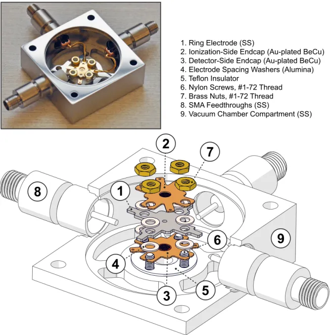
2.2.3 CIT Components . . . 63
2.3 Figures . . . 65
3 Experimental Results of CIT Geometry Optimization . . . 77
3.1 Overview of Studies . . . 77
3.1.1 Parameter Space . . . 78
3.1.2 Study Comparison and Optimization Routine . . . 81
3.2 Ancillary Geometry Concerns . . . 84
3.2.1 Effects of Endcap Mesh Size . . . 84
3.3 Experimental Considerations . . . 92
3.3.1 Competing Resolution Factors . . . 93
3.3.2 Buffer Gas Damping . . . 94
3.4 Results of High-Pressure Geometry Optimization . . . 97
3.4.1 Resolution as a Function of Pressure . . . 98
3.4.2 Resolution as a Function of Geometry . . . 102
3.4.3 Ion Storage Capacity . . . 105
3.5 Conclusions . . . 108
3.6 Figures . . . 111
4 Correlation of Performance with CIT Field Composition . . . 138
4.1 Higher Order Fields . . . 138
4.1.1 CIT Field Linearity . . . 139
4.1.2 Multipole Composition Determination . . . 140
4.1.3 Multipole Significance . . . 142
4.2 Individual Multipole Effects on Mass Analysis . . . 146
4.2.1 Spectral Resolution . . . 146
4.2.2 Supplementary Dipole Strength . . . 148
4.2.3 Field Linearity . . . 150
4.3 Simplification of Analysis . . . 151
4.3.1 Field Compensation . . . 151
4.3.2 Interpretations . . . 153
4.4 Combined Multipole Parameters . . . 155
4.4.1 Spectral Resolution . . . 156
4.4.2 Supplementary Dipole Strength . . . 158
4.4.3 Survey of Geometry Optimization Results . . . 160
4.5 Characteristics of Double-Resonance Ejection . . . 162
4.7 Octopole Effects on Ion Storage Capacity . . . 166
4.8 Conclusions . . . 167
4.9 Figures . . . 169
5 Conclusions and Future Directions . . . 202
Appendix A: Stability Parameter Approximations . . . 208
Appendix B: Multipole Coefficients for Evaluated CIT Geometries . . . 210
LIST OF FIGURES
1.1 Structure and potential contours of the QIT following the r02 2z
02
relationship with electrodes truncated at 2.5r0 along asymptotes . . . 47
1.2 Extended Mathieu stability diagram for the QIT in terms of au and qu parameters . . . 48
1.3 Enhanced view of the stability region that is most practical for mass analysis, labeled A in Figure 1.2 . . . 49
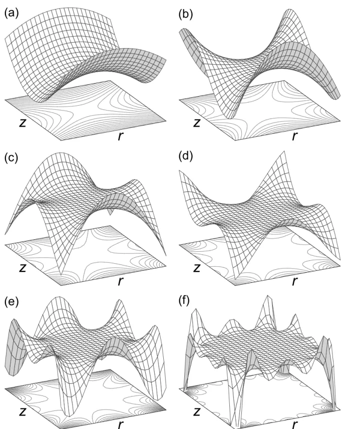
1.4 Potential surfaces and projected contour lines of a few pure multipole terms of order n computed from the general potential in eq 1.33 . . . 50
1.5 Predicted even-order nonlinear resonances for ν 1 . . . 51
1.6 Predicted odd-order nonlinear resonances for ν 1 . . . 52
1.7 Structure and potential contours of the CIT . . . 53
⁂ 2.1 Basic schematic diagram of electrical system components and wiring to perform mass analysis with the CIT . . . 65
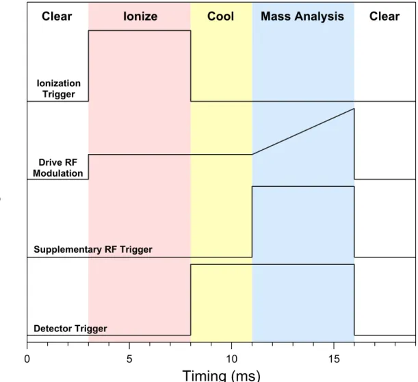
2.2 A typical timing diagram to perform a single mass analysis scan with the various MS components, with the different stages labeled . . . 66
2.3 Qualitative effects of averaging on mass spectra, showing improved repeatability with larger sample sizes . . . 67
2.4 Statistical analysis of each set of ten spectra from Figure 2.3 . . . 68
2.5 Diagrams of the electrical systems used for generating and applying the drive RF to the ring electrode and the supplementary RF to the endcaps . . . 69
2.6 Qualitative effects of drive RF amplitude instability on mass spectral performance . . . 70
2.7 Schematic of the vacuum and pressure-control system used for the high-pressure experiments . . . 71
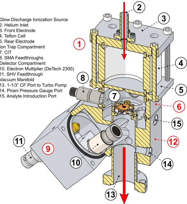
2.8 Drawing of the differential pressure vacuum chamber used for the high-pressure geometry optimization study . . . 72
2.10 Photograph of a gold-plated ionization-side endcap electrode with a
200 WPI TEM grid soldered over the central 2.5 mm diameter aperture . . . 74
2.11 Typical ring electrode diameter and concentricity measurements . . . 75
2.12 ESEM image of typical ring electrode surface finish within the
cylindrical cavity from the reaming and lapping fabrication process . . . 76
⁂
3.1 CIT geometry optimization parameters for a fixed r0 size . . . 111
3.2 CIT geometry optimization parameter space, relating the ring
thickness and electrode spacing to the dominant multipole terms, the
octopole and the dodecapole . . . 112
3.3 CIT geometry optimization parameter space with respect to the sum of
the octopole and dodecapole coefficients relative to the quadrupole. . . 113
3.4 Peak shifting phenomenon exhibited by CITs employing mesh endcaps
with small wire sizes . . . 114
3.5 Effects of mesh endcap wire density on spectral resolution, showing
only minor differences even with very coarse size . . . 115
3.6 Boundary ejection performance of CIT with 75 WPI mesh endcaps; the
two spectra were collected under identical conditions except that the trap was reassembled (after collecting red spectrum) with the endcaps
shifted laterally . . . 116
3.7 Endcap configurations and relative positions used in the trap electrode
alignment study . . . 117
3.8 Mass spectra collected with the traps described in Figure 3.7 in the
double-resonance mode of ejection utilizing the octopolar nonlinear
resonance near βz 0.70 . . . 118
3.9 Nonlinear resonance map obtained experimentally for the ‘misaligned’
aperture endcap trap detailed in Figure 3.7a(2) by sweeping the
frequency of the supplementary dipole field . . . 119
3.10 Mass spectra collected in the boundary ejection mode to confirm the
presence of a strong nonlinear resonance near βz 0.84 that can cause
spurious ejection when an aperture endcap is misaligned . . . 120
3.11 Mass spectra of anisole collected at variable drive frequencies in
3.12 Typical effects of mass scan rate on mass resolution and analysis time
at variable buffer gas pressures . . . 122
3.13 Peak width increase with pressure at different drive frequencies and
buffer gas species . . . 123
3.14 Mass spectra collected in the boundary ejection mode to qualitatively
illustrate the shifting of the βz 1 stability boundary to lower qz values
with increase in helium background pressure . . . 124
3.15 Quenching of double-resonant ejected peaks when background gas pressure is increased without a corresponding increase in the
supplementary RF amplitude . . . 125
3.16 Effects of tuning the supplementary RF amplitude on peak width under
double-resonance ejection mode at βz 0.70 for traps where
A4/A2 A6/A2 was greater than ca. −11% . . . 126
3.17 Unfavorable tuning results of supplementary RF amplitude exhibited
by traps where A4/A2 A6/A2 was less than ca. −11% . . . 127
3.18 Typical example of mass spectral changes observed with increase in
helium buffer gas pressure in different mass analysis modes . . . 128
3.19 Mass spectral peak widths obtained for all tested geometries in the double-resonance ejection mode of mass analysis via the octopole
nonlinear resonance near βz 0.70 . . . 129
3.20 Mass spectral peak widths obtained in the boundary ejection mode for
some tested trap geometries . . . 130
3.21 The best spectral resolution obtained with the dodecapole nonlinear
resonance at βz 0.522 (from the 2βr βz 1 condition) in the double
resonance ejection mode . . . 131
3.22 Correlation of geometry optimization results to the z0/r0 ratio . . . 132
3.23 Contour plots of peak width (FWHM) variation in the
double-resonance ejection mode near βz 0.70 for CITs with different ring
thicknesses and electrode spacing . . . 133
3.24 Contour plot of slopes of the curves in Figure 3.19 at pressures above ca. 250 mTorr where the peak width increases linearly with pressure
for most geometries . . . 134
3.25 Contour plot of peak widths (FWHM) obtained in the boundary
3.26 Two possible methods for quantifying the spectral space charge limit
with CITs . . . 136
3.27 Space-charge-limited ion storage capacity of CITs as a function of z0 . . . 137 ⁂
4.1 Axial electric field linearity for trap geometries from the high-pressure
optimization study in terms of the ring thickness and electrode spacing
parameters . . . 169
4.2 Qualitative view of fitting accuracy relative to number of terms
included in multipole expansion equation . . . 170
4.3 Individual multipole components of the axial electric field Ez for a
typical CIT . . . 171
4.4 Axial electric field strength of the octopole (A4), dodecapole (A6), and
hexadecapole (A8) for all 20 of the geometries evaluated in the
high-pressure optimization study . . . 172
4.5 Surface plots of coefficient values for the octopole (A4), dodecapole
(A6), and hexadecapole (A8) fields relative to the quadrupolar term (A2)
across a broad range of ring thickness and electrode spacing
parameters . . . 173
4.6 Expanded view of coefficient values (given as %A2) in contour plot
format, taken from the gray inner box of Figure 4.5 . . . 174
4.7 Contour plots of peak width (FWHM) variation for CITs with different
octopole and dodecapole compositions . . . 175
4.8 Contour plots with same peak width data and format as those in
Figure 4.7, except showing variation with the hexadecapole coefficient
values of the CITs on the vertical axis . . . 176
4.9 Contour plots of slopes of the curves in Figure 3.19 at pressures above
ca. 250 mTorr. Both panels show trends with A4 coefficient on abscissa,
with A6 on ordinate of (a) and A8 on ordinate of (b) . . . 177
4.10 Contour plots of peak widths (FWHM) obtained in the boundary ejection mode at 20 mTorr. The octopole coefficient values lie on the abscissa of both panels; the ordinate of (a) shows trends with the
dodecapole, while the hexadecapole values are given in (b) . . . 178
4.11 Contour plots of required supplementary dipole field strengths
(Vp‑p/mm) to start resonantly ejecting ions near βz 0.70 (the octopolar
nonlinear resonance) at different helium background pressures, as a
4.12 Axial electric field linearity as a function of the octopole and
dodecapole field strengths . . . 180
4.13 Calculated axial electric field strengths for pure quadrupole (A2),
octopole (A4), and dodecapole (A6) terms, with different coefficient
weights applied to the dodecapole . . . 181
4.14 Axial electric field strengths of superimposed octopole and dodecapole terms as calculated from the coefficients determined for the traps from
the high-pressure geometry optimization study . . . 182
4.15 Axial electric fields of the CITs from the high-pressure geometry study
compared to the ideal linear quadrupole field . . . 183
4.16 Variation of axial electric field strength with endcap (EC) aperture size
in a CIT, compared to the linear field of an ideal quadrupole . . . 184
4.17 Two methods of relating the octopole and dodecapole field strengths
for the purposes of identifying conditions for best performance . . . 185
4.18 Trends in peak width from the high-pressure geometry optimization study as a function of the sum of the octopole and dodecapole
coefficients . . . 186
4.19 Same as Figure 4.18 except showing peak width trends versus the ratio
of the octopole and dodecapole coefficients . . . 187
4.20 Same as Figure 4.18 except showing peak width trends versus the
strength of the octopole field relative to the quadrupole . . . 188
4.21 Correlations of the octopole-to-dodecapole coefficient ratio to (a) the strength of the octopole relative to the quadrupole and (b) the sum of
the octopole and dodecapole coefficients . . . 189
4.22 Correlation of supplementary dipole field strength that is required to
start ejecting ions via the octopolar nonlinear resonance (βz 0.70)
with combined weights of octopole and dodecapole coefficients . . . 191
4.23 Comparison of supplementary dipole field strength requirements at 20 mTorr for various mass spectral set points under octopolar
double-resonance ejection. . . 192
4.24 Peak width variation with helium background pressure, with the curve colors set according to the sum of the respective trap octopole and dodecapole coefficients to show trends based on the electric field
4.25 Contour plots of peak width data from Figure 4.24 showing trends versus background pressure and (a) the sum of the octopole and dodecapole coefficients, (b) the octopole-to-dodecapole ratio, and
(c) the weight of the octopole field alone . . . 195
4.26 Plot of resonance activity as measured through mass spectral peak
width in the resonance ejection mode over a range of βz ejection points . . . 196
4.27 Plot of resonance activity obtained in the same manner as Figure 4.26, except using a CIT with a ring thickness of 0.750 mm and electrode
spacing of 0.250 mm . . . 197
4.28 Plot of peak width versus helium background pressure in the
resonance ejection mode at two different βz ejection points (labeled) for
the CIT from Figure 4.27 . . . 198
4.29 Mass spectra obtained under different modes of mass analysis to
demonstrate the effect of the hexapole field on resolution. . . 199
4.30 Space-charge-limited ion storage capacity of CITs as a function of the
strength of the octopole field . . . 200
4.31 Surface plots (with projected contour lines) of magnitude of electric field from the superposition of a pure quadrupole with a pure positive
LIST OF TABLES
B.1 Raw values of multipole expansion coefficients for mesh-endcap CIT
geometries tested at high pressure . . . 210
B.2 Relative multipole expansion coefficient values for mesh-endcap CIT
LIST OF ABBREVIATIONS AND SYMBOLS
ABBREVIATIONS:
2D Two-dimensional
3D Three-dimensional
AC Alternating current
CF ConFlat (flange)
CIT Cylindrical ion trap
DAPI Discontinuous atmospheric pressure interface
DAQ Data acquisition (system)
DC Direct current
EI Electron (impact) ionization
EM Electron multiplier
FT-ICR Fourier transform ion cyclotron resonance
FWHM Full width at half maximum
GC Gas chromatograph(y)
GD Glow discharge
HMCO High-mass cutoff
HPMS High-pressure mass spectrometry
LIT Linear ion trap
LMCO Low-mass cutoff
MS Mass spectrometry
QIT Quadrupole ion trap
RF Radio frequency
SMA Subminiature version A (RF connector)
S/N Signal-to-noise ratio
SWaP Size, weight, and power
TOF Time of flight
LATIN SYMBOLS:
A Normalized potential difference between electrodes
An Multipole weighting coefficient
C Fixed floating potential or offset
z
D Pseudopotential well depth in the axial trap dimension
e Charge of ion in coulombs
E Electric field vector
Ez Electric field component in the axial dimension
F Force vector
fd Ordinary drive frequency in hertz
Fz Component of force in the axial dimension
m Ion mass
m/z Mass-to-charge ratio of an ion
Pn Legendre polynomial of order n
q Charge of particle in coulombs
qu Dimensionless Mathieu stability parameter in u dimension
r0 Radius of the ring electrode
Sn Dimensional weighting factors t Time
u Coordinate dimension in x, y, z or r
U DC voltage
V Amplitude of AC (RF) voltage
z0 Axial distance from the center of a trap to the apex of an endcap electrode
GREEK SYMBOLS:
βu Dimensionless trapping parameter in the u dimension
θ Polar angle
ξ Dimensionless phase or time interval
ρ Radial distance in the spherical coordinate system
ρmax Maximum ion density
φ Azimuthal angle
Electric potential
0 Potential applied to the ring electrode
ωu,n Secular frequency in u dimension of order n
ωz, ωz,0 Fundamental axial secular frequency
Ω Angular drive frequency
SPECIAL UNITS:
Th Thomson, unit of m/z, defined as Da/e (daltons per elementary charge)
V0‑p Zero-to-peak amplitude of an AC potential
Vp‑p Peak-to-peak amplitude of an AC potential
CHAPTER 1
INTRODUCTION
The search for balance between capability and convenience is not a new struggle.
This age-old equation persists because practicality usually places the variables at odds with
each other. When an imbalance is created out of necessity, it can be corrected by shifting
the fulcrum through advances in science and technology. It is interesting to consider, then,
that while we no longer depend on horses for transportation or homing pigeons for
communication, there is still widespread use of trained dogs for chemical detection.
When it comes to analytical instrument development, the traditional mindset of
lab-based analysis is primarily concerned with figures of merit, without placing much emphasis
on the footprint. Hence, decades of research have led to great improvements in
performance, but without broadening accessibility outside the lab environment or
increasing affordability. Long-standing centralization of specialized equipment and
personnel largely restricted chemical analysis to these locations, with little recourse for
remote or unique samples. However, bolstered by the fabrication tools from the
microelectronics industry, a new movement began near the end of the twentieth century to
redesign instruments into smaller, faster, and more efficient systems.
This new frontier in analytical chemistry is in the process of expanding the
discipline in many respects, already encompassing a variety of techniques.1 Among these,
mass spectrometry (MS) is poised to offer the advantages it has in the laboratory to a new
the characteristic ion fragmentation patterns provide detailed structural information. High
sensitivity is readily achieved when mass analyzers are coupled with detectors such as
electron multipliers. Additionally, a wide variety of ionization sources have been developed
to accommodate diverse compounds across samples of ranging complexity. Even though
the concept of miniature MS spans decades, with a number of commercial models already
available, much work remains in adapting the components into a convenient form factor
while closing the gap in performance compared to established systems.
This dissertation is focused on a few aspects of a specific mass analyzer — the
cylindrical ion trap (CIT). It is one of many forms in the general family of ion trap mass
analyzers, which are collectively among the most promising candidates for handheld MS.
The remainder of this chapter gives a brief review of miniature mass spectrometers, then
covers some essential background theory and principles to provide a clear perspective for
the project objectives stated at the end, while the next chapter explains the methods and
instrumentation employed in this study. Chapter 3 contains the experimental results of
optimizing the CIT geometry for high-pressure operation, including some considerations of
secondary geometric features and other factors affecting resolution. This is followed by
analysis in Chapter 4 with regards to the electric field composition in order to generalize
the results across different trap structures. Chapter 5 closes with conclusions and the future
outlook of this work.
1.1 The Mobilization of Mass Spectrometry
The ideal portable mass spectrometer would be no more of a burden to carry than a
modern cell phone while providing unquestionable specificity and rapid answers to the
searching and screening for explosives, and urgent medical diagnostics. Mitigating
imminent threats is only the beginning of a long list of applications that would benefit from
this device, including the monitoring of industrial production lines, tracking pollutants,
mineral exploration, forensics, and the identification of possible contraband substances.
These all share common concerns regarding sampling. In some cases, results are needed on
the spot and there is insufficient time to transport the sample to a distant facility. In others,
the sample may be unstable or difficult to collect, or perhaps the time and manpower
required are simply cost-prohibitive. Whatever the reason, the alternative approach to
conventional sampling is to bring the mass spectrometer to the field for in situ analysis.
1.1.1 General Developments
Perhaps the most extreme example of sampling involves remote extraterrestrial
analysis by unmanned vehicles. In this case, sending an instrument to make measurements
on-site is preferable to facing the logistics and expense of recovering a multitude of
samples, with the added risk of contamination. Due to the high costs of carrying a payload
into space, there are clear advantages to having the smallest and lightest instrument
possible. In fact, the need to perform mass spectral analysis on such missions is one of the
earliest driving forces for transforming standard laboratory instruments so they can be
taken into the field. In the mid-1970s, NASA’s Viking program launched two probes to
study the atmosphere and soil composition of Mars.2 Each of these had a sector mass
spectrometer on board, coupled with a gas chromatograph (GC).3
Further development was slow until interest picked up in the 1990s to study the
miniaturization of existing mass analyzers, with focus shifting the following decade
Throughout this time, various degrees of portability have been achieved. As defined by
Lammert,4 a transportable system is one that is detached from its environment but must be
conveyed on wheels (vehicle or cart) or carried by a few people. A person-portable system is
small enough to be carried by a single individual, as in a backpack. The smallest system is
hand-portable, only imposing a minor load and easily added as an accessory item. This
range exists because of the inherently inverse relationship between performance and the
instrument’s size, weight, and power consumption (SWaP). Since it is not yet possible to
have the best of both worlds in one package, tradeoffs must be made, and thus a spectrum
of tailored devices is necessary to meet demand.
In order for the device to remain useful, the performance cannot be overly
compromised for the sake of portability, and vice versa. A balance point can be reached by
setting the target performance according to the minimum requirements of the intended
application. For example, in many cases unit mass resolution would be sufficient, which
greatly eases many of the engineering difficulties of a hand-portable system. Resolution
concerns can be lowered further by employing automated statistical analysis and reference
libraries. This is a good solution when the detection of a limited number of analytes is
needed with high throughput — a low rate of false negatives can be maintained while
relying on relatively crude raw data. Another advantage of such processing is that one of
the largest and most expensive elements of an MS system becomes optional: the skilled
technician who usually interprets the data. An obvious drawback, however, is decreased
versatility.
Portable MS has not yet been widely adopted, pending better solutions to industry
problems. A variety of challenges remain to be solved, centered on the mass analyzer but
shrinking the mass analyzer does not generally translate to a reduction in SWaP for the
other hardware, which includes the ionization source, detector, electronics, and pumps.
Power is itself ultimately another manifestation of size and weight in miniature systems. It
has little bearing when drawn from an outlet, but becomes a scarce resource when supplied
by batteries. Given the present limitations of energy storage technology, batteries are still
among the largest and heaviest parts.
1.1.2 Strategies for Inadequate Pumps
The vacuum system is typically the most expensive and difficult to manage in terms
of SWaP. Consequently, its design and shortcomings are the primary obstacles in miniature
MS research. There are currently no satisfactory pumps available with the necessary
specifications for a hand-held device that can maintain the high vacuum conditions usually
required in a mass spectrometer (well below 10−3 Torr), although there are some
commercial options for less portable purposes.5 As long as pumping capacity remains
deficient, alternative strategies must be employed to undertake MS under the constraints of
existing pumps. For mass analyzers that depend on low pressure to achieve good
performance, the gas load imposed by sample introduction can be reduced in one of two
ways. Under continuous operation with a constant gas stream, a smaller orifice can be used
at the inlet for lower conductance. However, the smaller flow rate directly affects the ion
throughput and thus the sensitivity.6,7 Conversely, a discontinuous atmospheric pressure
interface (DAPI) can be used to pulse the gas in short bursts between longer pump-down
segments.8,9 Although sensitivity isn’t curtailed during the brief low-pressure period when
analysis is possible, this cyclical action makes DAPI unsuitable for high sampling rates,
somewhat by implementing a vacuum tethering strategy: the device is initially evacuated at
some designated station, after which vacuum is maintained for a limited period of time by a
small pump such as an ion getter. In this interval the spectrometer is free to be transported
as needed, with the caveat that it is not self-sustaining. A pulsed sample introduction
method akin to DAPI must be used to avoid overwhelming the pumps. In some
circumstances a semipermeable membrane may be a good solution for continuous sampling
without exceeding pumping capacity, but its chemically selective nature precludes general
use.11,12
To circumvent the issues of modest pumping technology, a profoundly different
approach can be taken to system design. The goal of high-pressure mass spectrometry
(HPMS) is to perform mass analysis entirely at the elevated pressures typical of such
pumping conditions (100 mTorr).13 This means that each component of the system must
be capable of operating at high pressure, with unique hurdles presented for the ionization
source, detector, and the mass analyzer. This dissertation is a continuation of previous
work in this group based on the HPMS strategy.
1.1.3 Ion Sources for HPMS
Electron ionization (EI) is a commonly used technique for converting neutral
analytes into positively charged ions, particularly for organic compounds. The traditional
electron source is a resistively heated filament combined with accelerating and focusing
potentials to direct the beam as needed. These thermionic emitters are inappropriate for
HPMS, the foremost reason being their incompatibility with high pressures, especially if air
is the background gas. Due to the extreme temperatures involved they are subject to rapid
for relatively high power consumption. A glow discharge (GD) source, on the other hand, is
a good alternative. They are intrinsically suited for high pressure conditions and can be
operated in EI mode by extracting electrons from the plasma.14 With occasional cleaning
their lifetime is indefinite, and power draw is a slight fraction of a hot cathode’s. There is
ongoing research into next-generation field effect sources based on novel materials and
microfabricated structures to further improve ionization efficiency and reduce power
consumption to negligible levels.15
Although the aforementioned internal ionization sources are ideal for volatile
samples, they are not the best choice for field applications due to their comparatively low
throughput. Ambient ionization techniques paired with atmospheric pressure interfaces
enable the analysis of samples in their natural state with no prior workup and are
applicable to nonvolatile substances. Desorption electrospray ionization (DESI)16 and direct
analysis in real time (DART)17 are well-known options. When constrained by poor
pumping speed, these ion sources face heavy disadvantages in non-HPMS systems (from
workarounds such as DAPI).
1.1.4 Detectors for HPMS
A pressure-tolerant detector is also necessary to successfully conduct HPMS. The
most sensitive ion detectors are electron multipliers, providing gains on the order of 107
before any electronic amplification of the signal takes place. Unfortunately, they are also
inherently not fit for pressures much above 10−6 Torr. When this threshold is exceeded, ion
feedback from secondary electrons colliding with residual gas begins to increase noise
few versions have been designed expressly for miniature MS operation into the 10−2 Torr
range, but this is still insufficient for HPMS.
For trapped-ion mass analyzers where periodic motion of the ion is relatable to its
mass, image current detection can be implemented with Fourier transformation to convert
the measured frequencies into a mass spectrum, with no added risk of electrical breakdown.
In ultra-high vacuum conditions this method has given tremendous resolving power to
some mass analyzers, namely Fourier transform ion cyclotron resonance (FT-ICR)19 and the
orbitrap.20 It is nondestructive and thus extended ion re-measurement increases the
number of samples and leads to superior frequency resolution. Yet, coherent pickup is
impaired at high pressure — the ion collisions with neutrals destabilize periodicity.
Furthermore, the collapsing ion trajectories induce weaker currents in the detection
circuitry which decreases signal strength.21 The extended measurement time also translates
to slower data acquisition rates.
Another pressure-tolerant detection scheme is the Faraday cup, which uses a circuit
tied to a biased sensor electrode to amplify the charges that are transferred from impinging
ions. Except for their indifference to pressure, they are inferior to electron multipliers in
most respects. The gain is lower by many orders of magnitude, and narrow bandwidth can
distort peak shape. Nonetheless, for HPMS they are currently the most viable choice.22,23
1.1.5 Pros and Cons of Common Mass Analyzers
Mass analyzers separate ions according to their mass-to-charge ratios (m/z) by
influencing their trajectories in space, time, or frequency using electric and/or magnetic
fields. The thompson (Th) is a unit of m/z, defined as Da/e (daltons per elementary
minimize the detrimental effects of ion-neutral collisions on performance. While a
reduction in analyzer size can decrease the total number of collisions at a given pressure by
shortening the ion pathlength, there is usually no further recourse to running it at greater
pressures. Moreover, in some analyzers the spatial confinement itself will adversely affect
resolution. Yet, at smaller dimensions all mass analyzers naturally need lower voltages to
maintain electric field strengths, which alleviates the strain on supporting electronics.
Beyond this, each analyzer holds special challenges, as well as benefits, and thus selecting
one for a miniature system has not been a straightforward process. As reported in 2000,
there was comparable representation from all common analyzers in miniaturization
research.25 By a 2009 review, however, the strong advantages of ion traps had emerged and
led to their commercial dominance,26 continuing to grow through the present. These
superior aspects are discussed in § 1.1.6 below.
Time-of-flight (TOF) analyzers are the simplest in regards to fabrication, consisting
of a field-free drift tube (although this is offset somewhat by the intricacies of the high
bandwidth detector and the injection of ions with uniform kinetic energy). While they
require high vacuum, this can be mitigated by shortening the tube and ion flight path, as
mentioned earlier. However, since mass resolution is intrinsically dependent on the length
of the tube, it strongly counters any miniaturization efforts of the TOF. Nevertheless,
working within these bounds, several systems have been produced. This includes small
benchtop units,27–29 several iterations of person-portable suitcase packages,30,31 and even a
micro-sized device with an integrated ion source and detector.32
Sector mass analyzers share the size-dependent resolution issue with TOF, and also
possess no special tolerance for rough vacuum conditions. Of the different possible
since it uses only static electric and magnetic fields, which makes it possible to implement
small permanent magnets and simple electronics. The associated simultaneous
transmission of all ions, rather than scanning them, lends itself to rapid data acquisition. As
a classic mass analyzer of widespread use, the sector was the first to attract attention for
miniaturization.25 Despite this, they have not been demonstrated as amenable to hand
portability, with interest waning after the turn of the century.33–36
The prevailing ambitions of FT-ICR development are in stark contrast with the
goals of miniaturization. To achieve maximum resolution, these instruments utilize ever
larger and more powerful superconducting magnets. A stringent vacuum is necessitated for
long and unperturbed ion lifetimes, otherwise the benefits of image current detection are
diminished. In spite of these detractors, a portable FT-ICR would be competitive even if it
retains just a slight fraction of the resolving power seen in its full form. While the practical
limit is still beyond hand-portability, a briefcase-sized device operating at 10−7 Torr with a
0.44 Tesla permanent magnet has been demonstrated with resolving power on the order of
500-1000.37,38
The quadrupole mass filter (QMF) is based on principles very similar to ion traps, in
that the physics governing ion stability have the same origin. The differences in electrode
configuration and operating parameters, however, clearly distinguish them in terms of
capability and performance. The QMF derives its name from the mass-selective stability
that ions have when traversing along two pairs of rods that confine them orthogonally via
RF (radio frequency) and DC potentials (which are scanned to pass single m/z values over
time). Consequently, it shares the drawbacks of other beam-type analyzers when it comes
to high-pressure operation. Although ion confinement in the radial plane features dynamic
With increased pressure, scattering caused by ion-neutral collisions prevents ions from
reaching the detector, lowering sensitivity. As with ion traps, though, the QMF is readily
parallelized; arrays of rods can be used to moderate lower sensitivity due to pressure and
other effects, such as space charge.39 While not as favorable as ion traps in many regards,
the QMF has wide market share, finding appeal particularly as a residual gas analyzer.40
These have been successfully tested up to 10 mTorr.41
It is worth mentioning the role of ion mobility spectrometry and its variants in the
history of portable detection, though it is distinct from mass spectrometry (separating ions
according to size and shape in addition to mass). As a predecessor that found popularity in
the 1990s among applications that miniature MS has also targeted, it suffers from high
false-positive rates amid background interferents due to its relative lack of selectivity. Yet,
they continue to rival MS in terms of sensitivity and detection limits, size, ease of use, and
response time.42–45
1.1.6 Advantages of Ion Trap Mass Analyzers
Ion traps have a broad set of advantages for portable MS, but what makes them
truly exceptional is their unique relationship with background pressure. Even without any
special adaptation for portable systems (i.e. at their normal laboratory scale) they not only
tolerate pressures that are many orders of magnitude higher than found in other analyzers,
they actually require them for optimal performance. This extends into the 1 mTorr range
for light buffer gas species such as helium, which are deliberately added for collisional
cooling effects. Kinetic energy is removed without scattering the ions, thereby collapsing
their trajectories to the center of the trap; this narrows their distribution and ultimately
frequency of the dynamic trapping field, which serves as an effective counterbalance.
Specifically, the resolving power is inversely proportional to pressure, but directly
proportional to drive frequency (see § 1.4.2). This compensation is the key enabling factor
of HPMS, opening the door to practical mass analysis at hundreds of millitorr. The
resulting high-pressure environment also reduces the extent of sample rarefaction,
increasing ionization efficiency and sensitivity.
Decreasing the size of an ion trap leads to a quadratic reduction in working voltage,
which translates to a quartic reduction in power. This is an important point considering
that HPMS pushes the frequency and voltage envelope to the limits of any RF amplifier that
is efficient enough for portability. Keeping the voltage in check is also essential because the
operating conditions of HPMS span a pressure regime that exacerbates electrical
breakdown. According to Paschen’s Law, the pressure-distance product for miniature ion
traps and their environments is near the minimum breakdown voltage for standard
background gases, which is made worse by RF potentials and smaller electrode radii.46,47
Ion storage capacity drops with trap size due to the mutual repulsion of like
charges. The induced space charge distorts the trapping potential and is deleterious to
performance long before saturation prevents the accumulation of any more ions (see
§ 1.2.5). However, these issues can be remedied by implementing large arrays of traps that
perform mass analysis in parallel.48–50 It is estimated that for a given footprint, an array of
n traps will have a factor of n1/2 greater capacity than a single trap occupying the same
area.51 Alternatively, instead of a uniform array, the trap elements can have a multiplex
configuration with varying specifications to expand the capabilities through flexible figures
of merit. For example, Misharin et al. have demonstrated a 4-channel design that is able to
On the other hand, arrays are more susceptible to degradation of resolution as a result of
fabrication or alignment imprecision. For nominally uniform arrays, trap-to-trap variability
contributes directly to electric field irregularity, causing ensemble peak broadening.
Therefore, arrays require tighter tolerances relative to a single trap to achieve the same
resolution.
Standard-sized ion traps are fairly small to begin with (having interior diameters on
the order of 2 cm) and prompt considerable concern towards tolerances in fabrication and
assembly. Miniaturization only aggravates the situation (enough to warrant manifold
research topics, including this present work). Although resolution is not fundamentally
limited by trap size, poor surface quality and faults in geometry and alignment will lead to
inferior performance. In order to avoid larger relative errors from a mechanical standpoint,
the absolute tolerances must improve in concert with trap size. Consequently, conventional
machining becomes unreliable for traps with features on scales under 1 mm. Although
micromilling tools can extend this range by another order of magnitude, these serial
production techniques are easily surpassed in terms of precision, time, and cost by
microfabrication technologies that have batch processing capabilities.
Ion traps can execute tandem MS studies within a single analyzer by virtue of
selective ion manipulation and partitioning the separation stages over time.11,53 Tandem MS
improves the overall selectivity and facilitates the analysis of more complex samples by
reducing chemical noise and augmenting structural elucidation methods. This ability and
the previously mentioned advantages are shared across an assortment of ion trap devices,
which can be classified by whether the ions are confined in a two- or three-dimensional
(2D or 3D, respectively) oscillating field. The 3D versions are rotationally symmetric, with
increases charge capacity proportionately. Axial ion injection along this line can also
significantly enhance trapping efficiency. For these reasons, 2D traps have superseded 3D
traps, despite arriving much more recently. The most common 2D variant, the linear ion
trap (LIT), utilizes additional static potentials at the ends to confine ions axially.54 In a
toroidal ion trap, the ends are joined to form a continuous circular track for ion
containment.55 Numerous geometric simplifications of all these exist as well.56–59
Almost all miniature ion trap systems are still designed for relatively low pressure
work and thus have not broken through the pumping barrier to achieve hand portability.
This excludes those that are based on a vacuum tethering strategy (discussed in § 1.1.2),
since that only temporarily bypasses the major SWaP constraints facing portable
spectrometers. For instance, the smallest ion trap MS reported to date employs this strategy
to attain a weight of just 1.5 kg and average power usage of 5 W, but with large tradeoffs in
sampling capability and performance.60 On the other hand, extensive development at
Purdue University has led to progressively smaller standalone instruments, namely the
Mini 10 (at 10 kg and 70 W) and Mini 11 (5 kg and 35 W) iterations.61,62 Of the sparse
published examples of portable MS in action, the Mini 10 underlines such utility with fast
analysis of toxic industrial compounds at detection limits well below permissible exposure
levels.63 Hyphenated instruments (which combine the selectivities of different analytical
techniques) are available commercially, with a 13 kg GC-MS offered by Torion in a suitcase
package.64 Other companies have focused on transportable benchtop solutions, such as the
MMS-1000 (8 kg) from 1st Detect65 and model 824 (23 kg) from Griffin Analytical.66 The
M908 from 908 Devices is currently the only hand-portable device to have put HPMS into
The HPMS approach is not clear-cut, of course, otherwise an ultraportable MS
solution would have emerged long ago and there would be no competition to meet today’s
needs. Although the intent has never been to compete with the performance level of
standard MS, the prospect of improvement will continue to drive research. To understand
how the interplay of the many ion trap parameters and conditions restrains the goals of
HPMS, it is necessary to review the guiding theory and principles of operation.
1.2 Ion Trap Theory
As discussed in the previous section, there are multiple ion trap designs. Due to
variations in structure and symmetry between 2D and 3D ion traps, there are some
differences in theory that have important consequences, particularly with regard to the
characteristics of their stability diagrams and relationships among nonlinear resonances.
Since the results presented in this dissertation deal only with 3D traps, the following
theoretical treatment is limited in scope accordingly. The reference works of March et al.
provide comprehensive coverage of these and many other ion trap topics.68–73
1.2.1 Origins and Structure
The invention of the 3D ion trap is credited to Paul and Steinwedel,74 who reported
it in 1953, although it took several decades of further development and serendipitous
discoveries before ion traps became popular in mass spectrometry (more so for versatility
than the relatively modest performance). In its more ideal form, the 3D ion trap is also
known as the quadrupole ion trap (QIT), where the name is derived from the quadrupolar
shape of the trapping potential established by the electrodes. Before describing it
physically, however, it is perhaps more informative to first consider the question of how a
chronological order of historical events surrounding ion traps, this approach starts with
basic principles to show a logical route to their conception. After examining the physics of
ion containment and determining the relevant stability parameters, it becomes apparent
that mass analysis is a natural extension and can be readily enacted.
As codified by Earnshaw’s theorem, it is not possible to trap a charged particle in
three dimensions by means of electrostatic fields alone.75 The static fields of the closely
related Penning trap (the basis of the FT-ICR) are not an exception, since a magnetic field is
used for confinement in two of the dimensions. It is, however, possible to confine ions by
means of an oscillating potential that imparts dynamic stability, alternating such that the
ions are focused towards a single point in space that is an effective, but not absolute,
potential energy minimum. For the sake of simplicity, harmonic ion motion is desired (this
allows an analytical expression to be derived that describes the motion in terms of stability
and frequency). The restoring force F acting on the ions, therefore, should increase linearly
with displacement r in any direction from a central point:
F r (1.1)
The next step is to determine the general form of the electric potential in 3D space that
will produce this condition. From the Lorentz force law in the absence of a magnetic field, a
particle of charge q in an electric field E will experience the force
q
F E (1.2)
Since the electric field is the gradient of the potential,
ˆ ˆ ˆ
or
x y z
a simple substitution shows that the force is related to the potential as
q
F (1.4)
It is clear, then, that in order for F to be linear as in eq 1.1, must be a quadratic function.
In Cartesian coordinates, the most general form of this potential is
2 2 2
1 2 3
( , , )x y z A S x( S y S z ) C
(1.5)
where A is the normalized potential difference between the electrodes, C is an adjustment
for any potential offset, and the Sn weighting factors along each dimension are associated
with the symmetry of the electrodes. It is reasonable to assume that the trapping volume
has negligible charge density; so, in order to satisfy Laplace’s equation for the potential,
2( , , ) 0x y z (1.6)
and given that A is non-zero, we find that the weighting factors must meet the condition
1 2 3 0
S S S (1.7)
The rotational symmetry of the QIT around the z axis dictates the equivalence of the x and
y dimensions, which can be accounted for by setting S1S2 1 and S3 2. In fact, for
convenience, we can convert to the cylindrical coordinate system using r2 x2y2
whereby the potential is then
2 2
( , )r z A r( 2 )z C
(1.8)
A direct way to establish a potential of this form is to shape the electrodes to follow
the equipotential contours, which means they should be hyperbolic surfaces. In practice,
three axially-symmetric electrodes are used, consisting of a central ring electrode that is
radial plane as shown in Figure 1.1a. The radius of the ring electrode is denoted as r0 and the axial distance from the center of the trap to the apex of an endcap electrode is denoted
as z0. Although the electrodes are constrained to share common asymptotes, Knight76
demonstrated that there are no restrictions on the relation between r0 and z0 and that the
general cross-sectional geometry follows
2 2 2
0
2
r z r (1.9)
for the ring electrode and
2 2 2
0
2 2
r z z (1.10)
for the endcap electrodes. However, it was common in the past to conform the dimensions
to the ratio of 2 2
0 2 0
r z since it was perceived to be ideal, if only to maximize the effective
confinement volume.77
To determine the values of constants A and C in eq 1.8 within the system of the
trap, the internal potential 0 is best defined as the relative difference in potentials applied
between the ring and endcap electrodes:
0 ring endcaps
(1.11)
In terms of eq 1.8 and the electrode boundaries we know that
2
0 0
( ,0) ( )
ring r A r C
(1.12)
and
2
0 0
(0, ) ( 2 )
endcaps z A z C
Substituting these into eq 1.11 and solving for A returns
0
2 2
0 2 0
A
r z
(1.14)
so that eq 1.8 becomes
2 2 0 2 2 0 0
( 2 )
( , )
2
r z
r z C
r z
(1.15)
Given that the QIT is typically operated with the endcaps at (or very near) ground
potential, such that we know (0, ) 0,z0 the constant C can be evaluated from eq 1.15 to
obtain the final form of the potential within the trap:
2 2 2
0 0 0
2 2 2 2
0 0 0 0
( 2 ) 2
( , )
2 2
r z z
r z
r z r z
(1.16)
The potential applied to the ring electrode can combine a DC voltage component U along
with an RF component of amplitude V (expressed as volts zero-to-peak, V0‑p) and angular
frequency Ω (equal to 2πfd where fd is the ordinary drive frequency in hertz) that alternates
over time t as a sinusoidal function:
0 U VcosΩt
(1.17)
The quadrupolar equipotential lines of eq 1.16 in the r-z plane are shown in Figure 1.1b for
a QIT that holds the 2 2
0 2 0
r z ratio.
1.2.2 Stability Parameters
Due to the absence of cross-dimensional terms in the quadrupolar potential, we are
movement of an ion of charge e and mass m in just the axial dimension at first, applying
eq 1.4 to the potential in eq 1.16 gives the z-component of force as
2 2
0 0
4 ( cosΩ )
2
z e U V t
F z
r z (1.18)
where eq 1.17 has been substituted for 0. To complete the equation of motion, this force
can be related to the ion’s acceleration by Newton’s second law,
22
z z d z
F ma m
dt (1.19)
so that we have the following second-order differential equation
2
2 2 2
0 0
4 ( cosΩ )
( 2 )
d z e U V t
z
dt m r z (1.20)
Equations of this class have been solved and applied in many areas of physics, so it
is convenient to simply adopt the corresponding solutions for this case. Specifically, eq 1.20
resembles the well-known Mathieu equation, which has the form
2
2 ( u 2 cos2 )u
d u
a q ξ u
dξ (1.21)
where qu and au are dimensionless stability parameters, u is a spatial coordinate, and ξ is a
dimensionless phase or time interval. Following the approach taken by March78 and others,
an exact conformation can be obtained by making the following transformation via the
chain rule
2 2
2 2 2
4
Ω
d u d u
and with a change of variables, whereby ξ is set to Ωt/2, so that eq 1.21 is rewritten as
2 2 2
2
Ω Ω cosΩ
4 u 2 u
d u a q t u
dt (1.23)
With a final expansion of eq 1.20,
2
2 2 2 2 2
0 0 0 0
4 4
cosΩ
( 2 ) ( 2 )
d z eU eV
t z
dt m r z m r z (1.24)
it becomes evident by direct comparison of eqs 1.23 and 1.24 that the stability parameters
for the QIT in the z dimension are
2 2 2
0 0
8
( 2 )Ω
z
eV q
m r z (1.25)
and
2 2 2
0 0
16
( 2 )Ω
z eU
a
m r z (1.26)
This exercise can be repeated for ion motion in the radial dimension, whereupon it is
determined that the stability parameters are related as 1
2
r z
q q and 1
2
r z
a a , stemming
from the values chosen for the weighting factors in eq 1.5.
For the present purpose, it is not necessary to investigate the complete integration
of the Mathieu equation, as would be needed to follow ion trajectories over time. The
nature of the solutions has been thoroughly characterized elsewhere79 in terms of the
stability parameters, and these general properties are sufficient to understand the
consequences for ion containment (and ultimately mass analysis, covered in § 1.2.4). As
they take different forms according to the values of qu and au. Unbounded solutions cause the ion trajectory amplitude to increase towards infinity from the center of the trap as ξ
increases, and are therefore unstable. Due to the finite boundaries of the physical trap,
these ions may either be neutralized after colliding with the walls of the electrodes, or they
may escape through holes that are incorporated for this reason. Bounded solutions for ion
motion are able to confine the oscillation amplitude within the trap volume, and are
therefore stable. This concept of stability is quantified by yet another dimensionless
parameter βu that is a function of qu and au (see § 1.2.3 below). Integer values of βu demarcate
the boundaries of stable and unstable motion, while rational non-integer values represent
stability; all other values of βu (i.e. complex numbers) are unstable.
These βu values can be used to map out domains of ion stability in qu and au space,
which are the coordinates of parametric plots referred to as stability diagrams (Figures 1.2
and 1.3). To improve readability, it is common to convert the radial stability parameters to
their axial counterparts qz and az so that they all lie in the same quadrants, which means
they are off by a factor of −2 in the diagrams. In order to be trapped in all dimensions, an
ion must reside in stable regions of βz and βr simultaneously by virtue of all the operating
variables embedded in the stability parameters. The most practical area of overlapping
stability is for 0 βu 1, which is the region closest to the origin, labeled A in Figure 1.2.
This is because the values of qu and au are directly proportional to the operating voltages V
and U, respectively. An expanded view of region A is shown in Figure 1.3; this stability
diagram is central to many ion trap concepts. Notably, the intersection of βz 1 with the
qz axis at qz 0.908 marks the lowest m/z ion that can theoretically be stored when
1.2.3 Frequencies of Ion Motion
Solutions of the Mathieu equation return a superposition of frequencies that
describe ion motion, also called the secular frequencies. This series can be calculated for
different orders of n (integer values) from already familiar terms:
1 2
, 1
2
( )Ω for 0
( )Ω for 0
u u n
u
n β n
ω
n β n (1.27)
where ωu,n necessarily has the same units as Ω. The magnitudes of the higher order
frequencies diminish quickly, so only those corresponding to values of n up to ±2 are
usually given consideration.69 The fundamental frequency components at n 0 are
predominant and outline the ion’s axial and radial harmonic oscillations that originate from
the quadrupolar potential surface. The axial secular frequency ωz,0 is of particular
importance in 3D traps since it is commonly used for the purposes of ion excitation,
selection, and manipulation; hereafter it will simply be denoted as ωz. Ions approaching the
βz 1 boundary will reach a maximum ωz of Ω/2 before becoming unstable. Under a fixed
set of operating conditions, ions of a given m/z will have secular frequencies unique from
other ions. On the stability diagram in Figure 1.3, iso-βu lines for intermediate values of βu
(between 0 and 1) delineate these conditions of constant frequency.
The accuracy of the calculated secular frequency depends on the accuracy with
which βu is known. Because there is no exact closed-form expression for βu in terms of qu
and au, the error level can only be lowered through iterative evaluations of the following
2 2 2 2 2 2 2 2 2 2 2 2 2 ( 2) ( 4) ( 6) ( 2) ( 4) ( 6) u u u u u u u u u u u u u u u u u u u u q β a q β a q β a β a q q β a q β a β a (1.28)
At sufficiently small values of qu and au (below 0.4), where ion motion can be treated as
consisting of simple harmonic oscillation in both r and z, an error of around 1% can be
achieved with the Dehmelt approximation:69
2 1 2
2
u u u
β a q (1.29)
More accurate approximations are provided in Appendix A, which are necessary for large
qu and au values; these were used to generate the stability diagrams presented here.
1.2.4 Modes of Mass Analysis
In the context of stability diagrams, an examination of the variables comprising the
stability parameters (eqs 1.25 and 1.26) makes it clear that ion confinement within the trap
is subject to experimental control. If the parameters of a stable ion are changed to unstable
values, the ion can be ejected from the trap through suitable apertures and steered to a
detector by means of external fields. To achieve this manipulation, it would be much less
practical to change the dimensions of the trap or the drive frequency than it is to apply
different voltages to the ring electrode. As per the earlier derivation, the endcaps are held
at ground potential in the modes discussed here, at least in regards to the trapping field.
Normally an axial stability boundary is employed so that ions are ejected only along this


![Figure 1.5 Predicted even-order nonlinear resonances for ν 1. The octopole resonances are [A] β r β z 1, [B] 2β r 1, and [C] 2β z 1](https://thumb-us.123doks.com/thumbv2/123dok_us/8241286.2184165/70.918.137.773.175.849/figure-predicted-order-nonlinear-resonances-octopole-resonances-c.webp)
![Figure 1.6 Predicted odd-order nonlinear resonances for ν 1. The hexapole resonances are [A] 3β z 2 and [B] 2β r β z 2](https://thumb-us.123doks.com/thumbv2/123dok_us/8241286.2184165/71.918.138.776.175.857/figure-predicted-odd-order-nonlinear-resonances-hexapole-resonances.webp)
![Figure 1.7 Structure and potential contours of the CIT. (a) Bisected trap showing the cylindrical cavity of the ring electrode [B] with radius r 0 and the planar endcap electrodes [A] and [C] separated by the distance 2z 0 about the center](https://thumb-us.123doks.com/thumbv2/123dok_us/8241286.2184165/72.918.180.696.109.846/structure-potential-contours-bisected-cylindrical-electrode-electrodes-separated.webp)