Linking in developmental scales

(1)

LINKING IN DEVELOPMENTAL SCALES

Michelle M. Langer

A thesis submitted to the faculty of the University of North Carolina at Chapel Hill in partial fulfillment of the requirements for the degree of Master of Arts in the Department of

Psychology.

Chapel Hill 2006

Approved by Advisor: David Thissen, Ph.D.

Reader: Daniel Bauer, Ph.D.

(2)

ABSTRACT

Michelle M. Langer: Linking in Developmental Scales (Under the direction of David Thissen, Ph.D.)

Developmental test score scales have attracted more interest with recent legislation on educational measurement, yet there remain a surprising number of unanswered

(3)

TABLE OF CONTENTS

Page

LIST OF TABLES...v

LIST OF FIGURES ...vii

Introduction...1

Literature Review...3

The National Assessment of Educational Progress (NAEP) and Developmental Scales...5

Empirical Differences Between Populations (for Different Grades)...7

Empirical Parameter Distributions...8

Study Design...9

Data Generation ... 10

Evaluation Criteria ... 11

Post-hoc Exploration... 12

Results ... 12

Mean Estimation for Small Mean Differences ... 13

Mean Estimation for Large Mean Differences ... 16

Standard Deviation Estimation for Small Mean Differences ... 18

Standard Deviation Estimation for Large Mean Differences ... 20

Conclusion ... 20

(4)

(5)

LIST OF TABLES

Table Page 1. Descriptive statistics for the NAEP 1988 Reading and 1990

Mathematics Assessments ... 23 2. Mean differences between grades for the 1988 NAEP Reading

Assessment and the 1990 NAEP Mathematics Assessment, expressed

in standard deviations for the lower grade... 24 3. Item parameter descriptive statistics for the 1998 NAEP Reading Assessment... 25 4. Mean bias in mean estimation by sample size for simulated mean

differences less than 3 standard deviations ... 26 5. Mean bias in mean estimation by simulated mean difference

(less than 3 standard deviations) ... 27 6. Regression model predicting bias in mean estimation for simulated

mean differences less than 3 standard deviations... 28 7. Regression model predicting bias in mean estimation with a quadratic

term for simulated mean differences less than 3 standard deviations... 29 8. Mean standard deviation of mean estimates by sample size for

simulated mean differences less than 3 standard deviations ... 30 9. Mean standard deviation of mean estimates by simulated mean

difference (less than 3 standard deviations) ... 31 10. Regression model predicting standard deviation of mean estimates for

simulated mean differences less than 3 standard deviations... 32 11. Regression model predicting standard deviation of mean estimates with

a quadratic term for simulated mean differences less than 3 standard deviations ... 33 12. Mean bias and mean standard deviation estimation of mean estimates

by sample size for simulated mean differences of 3 and 4 standard deviations ... 34 13. Mean bias and standard deviation of mean estimates by simulated mean

differences (3 and 4 standard deviations) ... 35 14. Regression model predicting bias in mean estimation for simulated mean

(6)

15. Regression model predicting standard deviation of mean estimates for

simulated mean differences of 3 and 4 standard deviations ... 37 16. Mean bias in standard deviation estimation by sample size for

simulated mean differences less than 3 standard deviations... 38 17. Mean bias in standard deviation estimation by simulated mean

difference (less than 3 standard deviations)... 39 18. Regression model predicting bias in standard deviation estimation for

simulated mean differences less than 3 standard deviations... 40 19. Mean standard deviation of standard deviation estimates by sample

size for simulated mean differences less than 3 standard deviations... 41 20. Mean standard deviation of standard deviation estimates by simulated

mean difference (less than 3 standard deviations) ... 42 21. Regression model predicting standard deviation of standard deviation

estimates for simulated mean differences less than 3 standard deviations ... 43 22. Mean bias and mean standard deviation of standard deviation estimates

by sample size for simulated mean differences of 3 and 4 standard deviations ... 44 23. Mean bias and mean standard deviation of standard deviation estimates

(7)

LIST OF FIGURES

Figure Page 1. Distributions of proficiencies for the 4th, 8th, and 12th grades and

locations of bparameters linking these grades on the 1988 NAEP

Reading Assessment ... 46 2. Distributions of proficiencies for the 4th, 8th, and 12th grades and

Mathematics Numbers and Operations Subscale... 47 3. Distributions of proficiencies for the 4th, 8th, and 12th grades and

Mathematics Measurement Subscale... 48 4. Distributions of proficiencies for the 4th, 8th, and 12th grades and

Mathematics Geometry Subscale... 49 5. Distributions of proficiencies for the 4th, 8th, and 12th grades and

Mathematics Data Analysis, Statistics, and Probability Subscale ... 50 6. Distributions of proficiencies for the 4th, 8th, and 12th grades and

Mathematics Algebra and Functions Subscale ... 51 7. Distribution of aparameters for the 1998 NAEP Reading Assessment ... 52 8. Distribution of bparameters for the 1998 NAEP Reading Assessment ... 53 9. Predicted value of bias in mean estimation, from regression model with

quadratic term, by sample size for simulated mean differences less than

3 standard deviations... 54 10. Predicted value of bias in mean estimation, from regression model with

quadratic term, by simulated mean difference (less than 3 standard deviations) ... 55 11. Predicted value of bias in mean estimation, from regression model with

quadratic term, by information for simulated mean differences less than

3 standard deviations... 56 12. Predicted value of standard deviation in mean estimation, from regression

(8)

13. Predicted value of standard deviation in mean estimation, from regression model with quadratic term, by simulated mean difference (less than 3

standard deviations) ... 58 14. Predicted value of standard deviation in mean estimation, from regression

model with quadratic term, by information for simulated mean differences

less than 3 standard deviations... 59 15. Predicted value of bias in standard deviation estimation by sample size

for simulated mean differences less than 3 standard deviations ... 60 16. Predicted value of bias in standard deviation estimation by simulated

mean difference (less than 3 standard deviations) ... 61 17. Predicted value of bias in standard deviation estimation by information

for simulated mean differences less than 3 standard deviations ... 62 18. Predicted value of standard deviation in standard deviation estimation

by sample size for simulated mean differences less than 3 standard deviations ... 63 19. Predicted value of standard deviation in standard deviation estimation

by simulated mean difference (less than 3 standard deviations)... 64 20. Predicted value of standard deviation in standard deviation estimation

(9)

Introduction

In educational testing, test batteries are used to measure student achievement throughout the school years. Each test in the battery may cover a wide range of content, including that which might have been taught to students in the earlier grades. The tests are typically given in levels (e.g., increasing difficulty with each grade) to increase the efficiency of the

measurement process. The developmental nature of the construct being measured implies a continuum, and student performance on the continuum may be evaluated at each grade by the use of a developmental score scale (Petersen, Kolen, & Hoover, 1989). By using the same metric for student performance in different age groups or grade levels, a developmental score scale permits test performance to be compared across levels and individual growth to be assessed in terms of changes in average performance and variability from grade to grade (Williams, Pommerich, & Thissen, 1998). The process of forming a developmental score scale is sometimes called vertical equating. Unlike horizontal equating which links test forms at a similar difficulty level, vertical equating links test forms that are intentionally different in difficulty (Skaggs & Lissitz, 1986).

(10)

within grades 10-12) by 2005-06, and adds a science assessment administered at least once in each of three grade spans by 2007-08. One of the common ways that psychometricians summarize the achievement of students is through developmental scales (Lissitz & Huynh, 2003).

Item response theory (IRT) has become a popular method of scaling educational

achievement tests. IRT describes the probability that examinees at different trait levels will correctly answer each item. An example of an IRT model is the three-parameter logistic (3PL) model, which assumes that the probability that an examinee with trait value will respond correctly to item iis

, ) ( )] ( 7 . 1 exp[ 1 1 i b i a i c i i c

P = + ₊

where aiis the item discrimination, biis the item difficulty, and ciis the lower asymptote.

The item parameters and trait values are estimated from examinees' responses to a set of items. Predictions based on the estimated parameters and traits are then compared to observed data to examine whether the model actually fits the data (Yen, 1986).

Given the significance of establishing valid developmental scales, there remain a surprising number of unanswered methodological questions. Little information is available on the number of common items needed to accurately link test forms across grades. Considering the cost of item development, such information is highly relevant. Furthermore, an

(11)

Can one link grades 4 and 8 or is the difference between the distributions of proficiency in those grades too large to be spanned with a single linking test? In addition, when selecting items to link grades, it makes logical sense to choose items with difficulty (b) parameters located between the means of the two grades. However, there is no guideline suggesting how many items need to have bparameters in that range and how many items could usefully fall outside that range.

Given these questions regarding the use of developmental scales, this study examined three primary questions. First, how many items are needed to accurately link a score scale across groups? Second, how large can the mean difference between groups be? Third, what locations are useful for the linking items’ bparameters?

Literature Review

To our knowledge, no research has considered the number of items required for vertical equating; however, several guidelines have been suggested for horizontal equating. Angoff's (1968, 1971) rule of thumb is to employ at least 20 items, or 20% of the items in the

(12)

individual testing program to decide what is an acceptable level of equating efficiency for its specific purpose, subject to time, cost, and context constraints.

These questions are also relevant for estimating population differences in a variety of contexts beyond the educational realm. Some research has been done on the suggested number of anchor items, analogous to a common item set, used with DIF methods. DIF analyses also require the estimation of the difference between distributions of groups with potentially different levels of proficiency. In educational measurement, the populations may be social groups; in health research, they may be pathological and nonpathological groups. In the context of DIF analysis, Thissen et al. (1988) evaluated 1, 4, and 50 anchor items and found that as the number of anchor items is increased, the power of DIF detection is also increased. Even one anchor item can yield satisfactory power. Wang and Yeh (2003) conducted a related study with 1, 4, and 10 anchor items, with a difference of 0.5 standard units between the population means. They drew a similar conclusion: although a single anchor item yields high power, 4 or 10 anchor items yield even higher power.

(13)

ratios of group standard deviations on the common items of less than .8 or greater than 1.2 tend to be associated with substantial differences among the results obtained using different methods (Kolen & Brennan, 1995).

The National Assessment of Educational Progress (NAEP) and Developmental Scales One context that provides a basis for the exploration of the use of developmental scales is NAEP's prior implementation of this methodology. NAEP was designed to report what students in American schools, both public and private, know and can do. When the

Educational Testing Service (ETS) became the NAEP contractor in 1983, it introduced scales based on IRT as a way of presenting results to the general public. The original NAEP scales allowed all students to be placed on a common scale even though none of the respondents take all of the items within the pool. NAEP reports its results using a linear transformation of the IRT proficiency variable, which is also interpretable as a number-correct score on a hypothetical 500-item test. Scores on this hypothetical test typically range between about 100 to 400 (Beaton & Johnson, 1992).

The decision to report NAEP results using developmental scales has been somewhat controversial. NAEP traditionally assessed 9, 13, and 17 year olds and then added

(14)

Assessment of eighth-grade mathematics, the eighth-grade mathematics data were scaled separately, and the scale differences for various demographic subgroups were compared to those from the developmental scales based on the national data for grades 4, 8, and 12. No substantial differences were found (Yamamoto & Mazzeo, 1992).

Budget constraints have also had an impact on the use of developmental scales in NAEP, by reducing the total number of items that can be administered (Linn & Dunbar, 1992). In the 1990 Mathematics exercise pool, of the 275 scaled items, 88, or 32%, were administered at more than one age/grade level. Eight items (9% of the 88 linking items) exhibited DIF among different age groups and were treated as separate items for each of the age groups (Haertel, 1991). Therefore only the remaining 79 items were used to link the item pools onto a common scale at the three age/grade levels.

(15)

Empirical Differences Between Populations (for Different Grades)

Given the cost of the substantial number of items thought to be required for linking, and the potential for misinterpretation, NAEP stopped using developmental scales after 1990. It is of interest to look at the scaling characteristics of the 1988 NAEP Reading assessment and the 1990 NAEP Mathematics assessment, when developmental scales were implemented, to create a base from which to explore the questions of this study. The means and standard deviations for the 1988 NAEP Reading assessment and the subscales of the 1990 NAEP Mathematics assessment are presented in Table 1. The mean differences between grades, in standard deviation units of the lower grade, for each scale are listed in Table 2. For Reading, the means for adjacent grades are about three-fourths of a standard deviation apart. For Mathematics, the means for grades 4 and 8 are about one and a half standard deviations apart, whereas the means for grades 8 and 12 are around three-fourths of a standard deviation apart. There is a good deal of variability among the mean differences.

(16)

Empirical Parameter Distributions

To explore the research questions listed above, simulated item response data may be used. However, to simulate data from the IRT model, item parameters are required. A useful way to simulate test data is to simulate tests, by drawing tests’ item parameters from suitable distributions.

To determine the distributions from which one draws the item parameters, a list of 2PL item parameters from the 1998 NAEP Reading Assessment was compiled. Tables of item parameters by scale and grade are reported in The NAEP 1998 Technical Report (Allen, Donoghue, & Schoeps, 2001). Summary statistics for the scales are presented in Table 3. Because the parameter distributions were similar across scales and grades, they were collapsed into one distribution of aparameters and one distribution of bparameters

(corresponding to the total line in Table 3). Empirical histograms and superimposed normal curves for these two distributions are depicted in Figures 7 and 8.

Examining the parameter densities, the distribution of aparameters generally appears to be symmetric and suggests that it could be approximated by a normal distribution. Across scales, the mean is 0.78, and the standard deviation is 0.26 (Table 3). Thus, similarly distributed aparameters could be drawn from a normal (0.8, 0.25) distribution.

(17)

Study Design

To answer the questions posed in the introduction, a simulation study was conducted. All data was simulated for binary items, without taking guessing into consideration. The results can be extended to using graded items because the graded model is analogous to having several binary items. The main study involved only linking items, items that are common among the grades. An ancillary study included noncommon items.

There were 112 cells for the main study. This was a result of varying the number of linking items, mean differences between groups, the location of the bparameters, and sample size. The number of linking items was 5, 10, or 20. This part of the study uses only linking items. The mean differences were 0, 0.5, 1, 2, 3, or 4 standard deviations (with both

populations having the same standard deviation). (Some conditions with mean differences of 3 and 4 standard deviations were included in the study to test the limits for reliable linking after linking performed sufficiently well for the mean difference of 2 standard deviations. These cells involved only 5 linking items, although the bparameter distribution [narrow or wide] and the sample size [N= 250, 500, 1000, or 2000] varied from cell to cell). To address the question of where items should be when linking two groups, the location of the b

parameters was either a narrow or a wide rectangular distribution. A different set of b parameters was used for every replication. The narrow rectangular distribution included b parameters between 0.5 standard deviations below the low mean and 0.5 standard deviations above the high mean. The wide rectangular distribution included bparameters between 1.5 standard deviations below the low mean and 1.5 standard deviations above the high mean. The aparameters were drawn from a normal (0.8, 0.25) distribution, reflecting the

(18)

= 250, 500, 1000, or 2000 simulees per group. For each simulation, sample size was the same for both groups. NAEP uses sample sizes around 3,000; however, that is a cluster sample with a smaller effective sample size.

An ancillary study involved 6 cells. Noncommon items were included in an effort to better define the aparameters for the linking items. As a result, the linking items should have functioned more effectively, producing better mean and standard deviation estimates. The number of noncommon items was 10 or 20. The number of linking items was 1, 5, or 10. The case of only one linking item was included to examine whether one item can provide the basis for linking groups, given the inclusion of noncommon items. These simulations used only central values for the mean differences, bdistributions, and sample size. The between group mean difference was 0.5 standard deviations. The bparameters were distributed within the narrow range. For the noncommon items, the bparameters were drawn from a normal (0.8, 0.6) distribution; that is, 0.8 standard deviations above the mean of each group. Sample size was 1,000 for each group.

Data Generation

The simulation began by drawing Nvalues for each simulee in each group, along with the item parameters for the linking and noncommon items. Data were then generated using the two-parameter logistic model (2PL) model, which assumes that the probability that an examinee with trait value will respond correctly to item iis

, )] ( 7 . 1 exp[ 1 1 ) ( i i b a i

P = ₊

where aiis the item discrimination, and biis the item difficulty. After data were generated

(19)

software (Thissen, 2001). This process of generating item parameters, Nvalues, simulee responses, and then estimating parameters and the mean difference between groups was repeated 1000 times for each cell in the simulation.

For some replications in cells with large mean differences, the estimated variance collapsed (went to zero), stopping the Bock-Aitkin algorithm. The estimates produced in these replications were not used in data analysis. These replications were labeled as “deficient cases” and a count was tabulated for each cell.

Evaluation Criteria

For each cell, root mean squared error (RMSE) for the estimated mean difference and standard deviation ratio (the focal group standard deviation divided by the reference group standard deviation of 1.0) was calculated to evaluate the performance of the linking. RMSE is the square root of the average squared difference between the true value and the recovered value. Often tests of statistical significance are avoided because sample sizes in simulation studies result in nearly every comparison being statistically significant, while not necessarily being practically significant.

(20)

where SE is the standard error of measurement, was used to encompass the number of linking items as well as the range of the bparameter distribution. The value of information used was the average of information at the two means. In future linking studies, information can easily be calculated to determine the reliability of the linking. The reciprocal square root of the information in the linking items was used to provide a basis for a linear relationship. Post-hoc Exploration

For the cells with simulated mean differences of 3 or 4 standard deviations, the estimated variance of the second group distribution sometimes collapsed to zero and the linking was unreliable. Including noncommon items was a possible solution to this problem. As a result, an additional 8 cells with simulated mean differences of 3 or 4 standard deviations were added to the study, involving only 5 linking items, 10 noncommon items, a narrow b distribution, and a sample size varying from cell to cell (N= 250, 500, 1000, or 2000 simulees per group).

Results

(21)

For cells with mean differences less than 3 standard deviations, the inclusion of

noncommon items did not make a substantial impact on the linking. For example, the bias in mean estimation for the cell with 5 linking items, no noncommon items, a narrow range for the bparameter distribution, a sample size of 500 per group, and a true mean difference of 0.5 standard deviations is -0.005; the bias in standard deviation estimation for this cell is 0.002. For the analogous cell with 10 noncommon items, the bias in mean estimation is -0.009, and the bias in standard deviation estimation is -0.008. The bias in mean estimation for the cell with 10 linking items, no noncommon items, a narrow range for the bparameter distribution, a sample size of 500 per group, and a true mean difference of 0.5 standard deviations is 0.003; the bias in standard deviation estimation for this cell is 0.003. For the analogous cell with 10 noncommon items, the bias in mean estimation is -0.013, and the bias in standard deviation estimation is -0.003. All of these values are very small, and the

differences in bias due to the inclusion of noncommon items are trivial. Mean Estimation for Small Mean Differences

Marginal means of bias in mean estimation, for simulated mean differences less than 3 standard deviations, are reported in Tables 4 and 5. The very small values of bias are negative, indicating that the estimated mean difference between groups is smaller than the simulated mean difference. This occurs because estimated values of the second group’s mean are limited by the difficulty of the items; if the majority of simulees are “correctly” endorsing the items, a type of ceiling effect results. Across the various sample sizes, bias is relatively consistent. However, the marginal means of bias increase (in the negative

(22)

To model these relationships as well as the effects of information, bias was regressed on the reciprocal square root of sample size, the simulated mean difference between groups, the reciprocal square root of information in the linking items, and the number of noncommon items. Regression statistics are reported in Table 6. As Table 6 indicates, these variables are collectively significant predictors of bias, F(4,97) = 82.7, p< .0001, together accounting for 77.3% of the variance. Despite the good fit of this model, regression residuals indicated curvature in the predicted value of bias as well as the simulated mean difference.

(23)

Marginal means of estimated standard deviation of the sampling distribution, for simulated mean differences less than 3 standard deviations, are reported in Tables 8 and 9. The

standard deviation decreases with greater sample size and increases with larger simulated mean differences. The rows with noncommon items appear to have slightly more random variance, but these values only reflect the means of 3 cells.

These relationships and the effects of information were incorporated in a regression model; standard deviation of the sampling distribution was regressed on the reciprocal square root of the sample size, the simulated mean difference between groups, and the reciprocal square root of information in the linking items. The number of noncommon items was not included in this regression model because it was a nonsignificant predictor. Regression statistics are reported in Table 10. As Table 10 indicates, collectively these variables significantly predict standard deviation, F(3,98) = 464.3, p< .0001, together accounting for 93.4% of the

variance. Although this model exhibited good fit, regression residuals indicated curvature in the predicted value of standard deviation as well as the simulated mean difference.

To model the curvature in the regression residuals, a quadratic term, the simulated mean difference squared, was added to the regression model predicting standard deviation.

Regression statistics are reported in Table 11. Collectively the variables significantly predict standard deviation, F(4,97) = 414.4, p< .0001, together accounting for 94.5% of the

(24)

predicting standard deviation from this regression model against sample size per group, shows that the model fits the steep negative trend in the marginal means for sample size well. Figure 13 indicates that the regression model’s predicted values of standard deviation for the various simulated mean differences also fits the marginal means for the simulated mean differences. This plot emphasizes the increase of standard deviation with larger simulated mean difference values. Figure 14, a plot predicting standard deviation from this regression model against information, indicates that greater amounts of information predict substantially less standard deviation. In general, these relationships are stronger than for the models predicting bias.

Mean Estimation for Large Mean Differences

Marginal means of bias in mean estimation, for simulated mean differences of 3 and 4 standard deviations, are reported in Tables 12 and 13. Across the various sample sizes, bias is consistently large. These values are also much greater than the corresponding values in Table 4 for simulated mean differences less than 3 standard deviations. The marginal means of bias are substantially larger for the simulated mean difference of 4 standard deviations versus the simulated mean difference of 3 standard deviations, as well as for the

corresponding values in Table 5 for simulated mean differences less than 3 standard deviations.

(25)

regression model, the simulated mean difference is a significant predictor of bias. This is the same result as the regression model without a quadratic term for simulated mean differences less than 3 standard deviations. Also similar to the model for smaller simulated mean differences, information is a significant predictor. However, the reciprocal square root of sample size is not a significant predictor of bias as in the model for simulated mean

differences less than 3 standard deviations. Nevertheless, comparisons should be made with caution because there were only 16 cells used in the regression analyses for simulated mean differences of 3 or 4 standard deviations versus the 102 cells used in the regression analyses for simulated mean differences less than 3 standard deviations.

Marginal means of the standard deviation of mean estimates, for simulated mean differences of 3 and 4 standard deviations, are reported in Tables 12 and 13. Across the various sample sizes, standard deviation is consistently large. These values are also much greater than the corresponding values in Table 8 for simulated mean differences less than 3 standard deviations. The marginal means of standard deviation are substantially larger for the simulated mean difference of 4 standard deviations versus the simulated mean difference of 3 standard deviations, as well as for the corresponding values in Table 9 for simulated mean differences less than 3 standard deviations.

To address these relationships as well as the effects of information, standard deviation was regressed on the reciprocal square root of sample size, the simulated mean difference

between groups, and the reciprocal square root of information in the linking items. Regression statistics are reported in Table 15. As Table 15 indicates, collectively these variables significantly predict, F(3,12) = 93.8, p< .0001, standard deviation, together

(26)

sample size is a significant predictor of standard deviation. This is the same result as the regression model without a quadratic term for simulated mean differences less than 3 standard deviations. Also similar to the model for smaller simulated mean differences, information and simulated mean difference are significant predictors.

Standard Deviation Estimation for Small Mean Differences

Marginal means of bias in standard deviation estimation, for simulated mean differences less than 3 standard deviations, are reported in Tables 16 and 17. The values of bias are negligible, ranging from 0.01 to -0.03. Across the various sample sizes, bias is relatively consistent. However, the marginal means of bias increase (in the negative direction) with larger simulated mean differences. There appears to be more bias in the rows with noncommon items, but these values only reflect the means of 3 cells. These trends are congruent with those in mean estimation.

(27)

simulated mean differences. This plot emphasizes the sharp increase of negative bias with larger simulated mean difference values. Figure 17, a plot predicting bias from this regression model against information, suggests that bias approaches zero with greater amounts of information.

Marginal means of estimated standard deviation of the sampling distribution, for simulated mean differences less than 3 standard deviations, are reported in Tables 19 and 20. The values of estimated standard deviation are relatively small, ranging from 0.03 to 0.15. Standard deviation decreases with greater sample size and increases with larger simulated mean differences. These trends are similar to those for the estimated standard deviation in mean estimation.

To model these relationships as well as the effects of information, standard deviation of the sampling distribution was regressed on the reciprocal square root of sample size, the

(28)

Standard Deviation Estimation for Large Mean Differences

Marginal means of bias in standard deviation estimation, for simulated mean differences of 3 and 4 standard deviations, are reported in Tables 22 and 23. Across the various sample sizes, bias in estimates of the standard deviation is consistently large. These values are also much greater than the corresponding values in Table 16 for simulated mean differences less than 3 standard deviations. The marginal means of bias are substantially larger for the

simulated mean difference of 4 standard deviations versus the simulated mean difference of 3 standard deviations, as well as for the corresponding values in Table 17 for simulated mean differences less than 3 standard deviations. For simulated mean differences of 3 and 4 standard deviations, the values of bias are too large to warrant regression models. Marginal means of standard deviation of the sampling distribution, for simulated mean differences of 3 and 4 standard deviations, are reported in Tables 22 and 23. Across the various sample sizes, standard deviation is consistently large, though decreasing with greater sample sizes. These values are also much greater than the corresponding values in Table 19 for simulated mean differences less than 3 standard deviations. The marginal means of standard deviation are substantially larger for the simulated mean difference of 4 standard deviations versus the simulated mean difference of 3 standard deviations, as well as for the corresponding values in Table 20 for simulated mean differences less than 3 standard deviations. As with bias for simulated mean differences of 3 and 4 standard deviations, the values of standard deviation are too large to warrant regression models.

Conclusion

(29)

of 0.5 standard deviations or less to achieve reliable linking. However, linking performed surprisingly well for mean differences of 2 standard deviations or less and with any number of linking items. Furthermore, means and standard deviations were fairly accurately

recovered despite variations in sample size, information in the linking items, location of b parameters, and the inclusion of noncommon items. Bias in both mean and standard deviation estimation was considerably reduced by greater information and smaller mean differences. Standard deviation of the sampling distribution in both mean and standard deviation estimation was substantially decreased by greater sample size and greater

information. A narrow distribution of bparameters and the inclusion of noncommon items also generally increased reliability in linking.

However, for simulated mean differences greater than 2 standard deviations, linking was unreliable. In these cases, the link between groups was not made some of the time. Bias was substantial in both mean and standard deviation estimation. Standard deviation of the

sampling distribution was also large in both mean and standard deviation estimation. Given these results, attempting to link groups with mean differences greater than 2 standard

deviations is not advised. However, situations when such a problem could arise may be quite rare; NAEP mean differences between grades as far apart as the 4th and 8th grades or the 8th and 12th grades were all less than 2 standard deviations.

(30)

(31)

Table 1

Descriptive statistics for the NAEP 1988 Reading and 1990 Mathematics Assessments

Assessment Grade Mean SD

1988 Reading 4 230.4 41.4

8 262.8 37.3

12 287.1 34.8

1990 Mathematics

Numbers and Operations 4 212.5 33.5

8 268.7 34.8

12 294.3 33.4

Measurement 4 221.7 33.5

8 261.3 43.3

12 294.2 37.2

Geometry 4 217 30.9

8 261.7 35.5

12 296.2 41.5

Data Analysis, Statistics,

and Probability 8 266.1 41.2

12 295.2 36.3

Algebra and Functions 4 215.5 31.5

8 264.2 36.8

12 296.7 37.1

(32)

Table 2

Mean differences between grades for the 1988 NAEP Reading Assessment and the 1990 NAEP Mathematics Assessment, expressed in standard deviations for the lower grade

Assessment 8th – 4th Grade 12th – 4th Grade 12th – 8th Grade

1988 Reading 0.78 1.37 0.65

1990 Mathematics

Numbers and Operations 1.68 2.44 0.74

Measurement 1.18 2.16 0.76

Geometry 1.45 2.56 0.97

Data Analysis, Statistics, and Probability

0.71

Algebra and Functions 1.55 2.58 0.88

(33)

Table 3

Item parameter descriptive statistics for the 1998 NAEP Reading Assessment

Scale Grade # Items aMean aSD bMean bSD

Reading for Literacy Experience

4 26 0.78 0.19 0.71 0.63

8 7 0.94 0.36 0.36 0.41

12 8 0.80 0.34 0.69 0.39

Reading to Gain Information

4 26 0.86 0.28 0.74 0.46

8 11 0.86 0.24 0.86 0.62

12 15 0.62 0.25 0.94 0.92

Reading to Perform a Task 8 14 0.74 0.19 0.87 0.57

12 15 0.69 0.19 1.01 0.69

(34)

Table 4

Mean bias in mean estimation by sample size for simulated mean differences less than 3 standard deviations

Sample Size Per Group

250 500 1000 2000

0 Noncommon Items

-0.0086 (N= 24)

-0.0083 (N= 24)

-0.0114 (N= 24)

-0.0128 (N= 24) 10 Noncommon

Items

-0.0203 (N= 3) 20 Noncommon

Items -0.0273 (N= 3)

Average -0.0086

(N= 24) (N-0.0114 = 30) (N-0.0114 = 24) (N-0.0128 = 24) 5 Linking Items -0.0121

(35)

Table 5

Mean bias in mean estimation by simulated mean difference (less than 3 standard deviations)

Simulated Mean Difference

0.0 SDs 0.5 SDs 1.0 SDs 2.0 SDs

0 Noncommon

Items (N-0.0003 = 24) (N-0.0040 = 24) (N-0.0079 = 24) (N-0.0289 = 24) 10 Noncommon

Items -0.0203 (N= 3)

20 Noncommon Items

-0.0273 (N= 3)

Average -0.0003

(N= 24)

-0.0079 (N= 30)

-0.0079 (N= 24)

-0.0289 (N= 24) 5 Linking Items -0.0015

(N= 8)

-0.0035 (N= 8)

-0.0073 (N= 8)

(36)

Table 6

Regression model predicting bias in mean estimation for simulated mean differences less than 3 standard deviations

Predictor Variable B S.E. t

Reciprocal Square Root of Sample Size

0.1519 0.0599 2.54**

-0.0130 0.0009 -14.14*

Reciprocal Square Root of Information in Linking Items

-0.0240 0.0047 -5.16*

Noncommon Items -0.0009 0.0002 -5.24*

Intercept (B0) 0.0061 0.0025 2.42**

Note. Model F(4,97) = 82.68, p< .0001. Model R2= 0.77. Degrees of freedom = 101 for the t-tests.

(37)

Table 7

Regression model predicting bias in mean estimation with a quadratic term for simulated mean differences less than 3 standard deviations

0.1516 0.0547 2.77**

-0.0005 0.0029 -0.18

Simulated Mean Difference Squared

-0.0060 0.0013 -4.51*

-0.0240 0.0042 -5.65*

Noncommon Items -0.0010 0.0002 -6.30*

Intercept (B0) 0.0031 0.0031 1.28

(38)

Table 8

Mean standard deviation of mean estimates by sample size for simulated mean differences less than 3 standard deviations

250 500 1000 2000

0 Noncommon Items

0.1343 (N= 24)

0.0933 (N= 24)

0.0654 (N= 24)

0.0470 (N= 24) 10 Noncommon

Items

0.1100 (N= 3) 20 Noncommon

Items (N0.1088 = 3)

Average 0.1343

(N= 24) (N0.0965 = 30) (N0.0654 = 24) (N0.0470 = 24) 5 Linking Items 0.1563

(39)

Table 9

Mean standard deviation of mean estimates by simulated mean difference (less than 3 standard deviations)

0.0 SDs 0.5 SDs 1.0 SDs 2.0 SDs

0 Noncommon Items

0.0683 (N= 24)

0.0718 (N= 24)

0.0828 (N= 24)

0.1171 (N= 24) 10 Noncommon

Items

0.1100 (N= 3) 20 Noncommon

Items (N0.1088 = 3)

Average 0.0683

(40)

Table 10

Regression model predicting standard deviation of mean estimates for simulated mean differences less than 3 standard deviations

3.0282 0.1008 30.03*

0.0188 0.0015 12.33*

0.1065 0.0074 14.31*

Intercept (B0) -0.0596 0.0042 -14.08*

Note. Model F(3,98) = 464.34, p< .0001. Model R2= 0.93. Degrees of freedom = 101 for the t-tests.

(41)

Table 11

Regression model predicting standard deviation of mean estimates with a quadratic term for simulated mean differences less than 3 standard deviations

3.0318 0.0930 32.62*

-0.0014 0.0049 -0.29

Simulated Mean Difference Squared

0.0097 0.0023 4.28*

0.1078 0.0069 15.69*

Intercept (B0) -0.0551 0.0040 -13.63*

(42)

Table 12

Mean bias and mean standard deviation of mean estimates by sample size for simulated mean differences of 3 and 4 standard deviations

250 500 1000 2000

Mean Bias -0.3145 -0.2751 -0.2730 -0.2670

Mean Standard

Deviation 0.4711 0.3563 0.2898 0.2378

(43)

Table 13

Mean bias and standard deviation of mean estimates by simulated mean differences (3 and 4 standard deviations)

3 SDs 4 SDs

Mean Bias -0.1147 -0.4514

Mean Standard

Deviation 0.2411 0.4364

(44)

Table 14

Regression model predicting bias in mean estimation for simulated mean differences of 3 and 4 standard deviations

-1.5821 1.4622 -1.08

-0.2197 0.0505 -4.35*

-1.7023 0.5718 -2.98**

Intercept (B0) 1.7822 0.3075 5.80*

(45)

Table 15

Regression model predicting standard deviation of mean estimates for simulated mean differences of 3 and 4 standard deviations

8.0620 0.7348 10.97*

0.1256 0.0254 4.95*

1.0121 0.2873 3.52**

Intercept (B0) -1.0757 0.1545 -6.96*

(46)

Table 16

Mean bias in standard deviation estimation by sample size for simulated mean differences less than 3 standard deviations

250 500 1000 2000

0 Noncommon Items

-0.0018 (N= 24)

-0.0035 (N= 24)

-0.0054 (N= 24)

-0.0069 (N= 24) 10 Noncommon

Items

-0.0129 (N= 3) 20 Noncommon

Items -0.0196 (N= 3)

Average -0.0018

(N= 24) (N-0.0060 = 30) (N-0.0054 = 24) (N-0.0069 = 24) 5 Linking Items -0.0007

(47)

Table 17

Mean bias in standard deviation estimation by simulated mean difference (less than 3 standard deviations)

0.0 SDs 0.5 SDs 1.0 SDs 2.0 SDs

0 Noncommon Items

0.0057 (N= 24)

0.0004 (N= 24)

-0.0050 (N= 24)

-0.0187 (N= 24) 10 Noncommon

Items

-0.0129 (N= 3) 20 Noncommon

Items -0.0196 (N= 3)

Average 0.0057

(N= 24) (N-0.0029 = 30) (N-0.0050 = 24) (N-0.0187 = 24) 5 Linking Items 0.0092

(48)

Table 18

Regression model predicting bias in standard deviation estimation for simulated mean differences less than 3 standard deviations

0.1752 0.0445 3.94*

-0.0109 0.0007 -15.92*

-0.0222 0.0035 -6.42*

Noncommon Items -0.0008 0.0001 -6.09*

Intercept (B0) 0.0088 0.0019 4.66*

(49)

Table 19

Mean standard deviation of standard deviation estimates by sample size for simulated mean differences less than 3 standard deviations

250 500 1000 2000

0 Noncommon Items

0.1106 (N= 24)

0.0794 (N= 24)

0.0556 (N= 24)

0.0386 (N= 24) 10 Noncommon

Items

0.1180 (N= 3) 20 Noncommon

Items (N0.1110 = 3)

Average 0.1106

(N= 8) (N0.1023 = 8) (N0.0732 = 8) (N0.0504 = 8) Note. Mean standard deviation of standard deviation estimates is included for the cells with 5 linking items because this matches the conditions for all cells with simulated mean

(50)

Table 20

Mean standard deviation of standard deviation estimates by simulated mean difference (less than 3 standard deviations)

0.0 SDs 0.5 SDs 1.0 SDs 2.0 SDs

0 Noncommon Items

0.0676 (N= 24)

0.0679 (N= 24)

0.0715 (N= 24)

0.0773 (N= 24) 10 Noncommon

Items

0.1180 (N= 3) 20 Noncommon

Items (N0.1110 = 3)

Average 0.0676

(N= 8) (N0.0871 = 8) (N0.0942 = 8) (N0.1010 = 8) Note. Mean standard deviation of standard deviation estimates is included for the cells with 5 linking items because this matches the conditions for all cells with simulated mean

(51)

Table 21

Regression model predicting standard deviation of standard deviation estimates for simulated mean differences less than 3 standard deviations

2.5009 0.0893 28.00*

-0.0038 0.0014 -2.84**

0.1427 0.0066 21.64*

Intercept (B0) -0.0525 0.0038 -14.00*

(52)

Table 22

Mean bias and mean standard deviation of standard deviation estimates by sample size for simulated mean differences of 3 and 4 standard deviations

250 500 1000 2000

Mean Bias -0.1360 -0.1202 -0.1168 -0.1178

Mean Standard

Deviation 0.2413 0.1887 0.1526 0.1319

(53)

Table 23

Mean bias and mean standard deviation of standard deviation estimates by simulated mean differences (3 and 4 standard deviations)

3 SDs 4 SDs

Mean Bias -0.0609 -0.1845

Mean Standard

Deviation 0.1413 0.2159

(54)

Figure 1

Distributions of proficiencies for the 4th, 8th, and 12thgrades and locations ofbparameters linking these grades on the 1988 NAEP Reading Assessment

100 200 300 400

0.

00

0.

02

0.

04

0.

06

0.

08

0.

10

D

is

tr

ib

ut

io

n of

S

cor

es

Links 4th & 8th

Links 8th & 12th

Links 4th, 8th, & 12th

(55)

Figure 2

Distributions of proficiencies for the 4th, 8th, and 12thgrades and locations ofbparameters linking these grades on the 1990 NAEP Mathematics Numbers and Operations Subscale

100 200 300 400

0.

00

0.

02

0.

04

0.

06

0.

08

0.

10

0.

12

D

is

tr

ib

ut

io

n of

S

cor

es

Links 4th & 8th

Links 8th & 12th

Links 4th, 8th, & 12th

(56)

Figure 3

Distributions of proficiencies for the 4th, 8th, and 12thgrades and locations ofbparameters linking these grades on the 1990 NAEP Mathematics Measurement Subscale

100 200 300 400

0. 00 0 .0 2 0 .04 0. 0 6 0 .0 8 0. 10 0. 1 2 D is tr ib ut io n of S cor es

Links 4th & 8th

Links 4th & 12th

Links 8th & 12th

Links 4th, 8th, & 12th

(57)

Figure 4

Distributions of proficiencies for the 4th, 8th, and 12thgrades and locations ofbparameters linking these grades on the 1990 NAEP Mathematics Geometry Subscale

100 200 300 400

0.

00

0.

0

2

0

.04

0.

06

0

.08

0

.10

0

.12

D

is

tr

ib

ut

io

n of

S

cor

es

Links 4th & 8th

Links 8th & 12th

Links 4th, 8th, & 12th

(58)

Figure 5

Distributions of proficiencies for the 4th, 8th, and 12thgrades and locations ofbparameters linking these grades on the 1990 NAEP Mathematics Data Analysis, Statistics, and Probability Subscale

100 200 300 400

0.

00

0.

02

0.

04

0.

06

0.

08

0.

10

D

is

tr

ib

ut

io

n of

S

cor

es

Links 8th & 12th

(59)

Figure 6

Distributions of proficiencies for the 4th, 8th, and 12thgrades and locations ofbparameters linking these grades on the 1990 NAEP Mathematics Algebra and Functions Subscale

100 200 300 400

0.

00

0.

02

0.

04

0.

06

0.

08

0.

10

0.

12

D

is

tr

ib

ut

io

n of

S

cor

es

Links 4th & 8th

Links 8th & 12th

Links 4th, 8th, & 12th

(60)

Figure 7

Distribution ofaparameters for the 1998 NAEP Reading Assessment

0.225 0.375 0.525 0.675 0.825 0.975 1.125 1.275 1.425 1.575

0 5 10 15 20 25

P e r c e n t

(61)

Figure 8

Distribution ofbparameters for the 1998 NAEP Reading Assessment

-0.75 -0.25 0.25 0.75 1.25 1.75 2.25 2.75

0 5 10 15 20 25 30 35

P e r c e n t

(62)

Figure 9

(63)

Figure 10

(64)

Figure 11

(65)

Figure 12

Predicted value of standard deviation in mean estimation, from regression model with quadratic term, by sample size for simulated mean differences less than 3 standard

(66)

Figure 13

(67)

Figure 14

Predicted value of standard deviation in mean estimation, from regression model with quadratic term, by information for simulated mean differences less than 3 standard

(68)

Figure 15

Predicted value of bias in standard deviation estimation by sample size for simulated mean differences less than 3 standard deviations. Predicted value is computed with the regression equation using the means of all other variables. The bars represent the RMSE of the

(69)

Figure 16

(70)

Figure 17

Predicted value of bias in standard deviation estimation by information for simulated mean differences less than 3 standard deviations. Predicted value is computed with the regression equation using the means of all other variables. The bars represent the RMSE of the

(71)

Figure 18

(72)

Figure 19

Predicted value of standard deviation in standard deviation estimation by simulated mean difference (less than 3 standard deviations). Predicted value is computed with the regression equation using the means of all other variables. The bars represent the RMSE of the

(73)

Figure 20

(74)

Appendix A

(75)

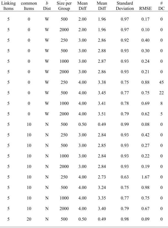
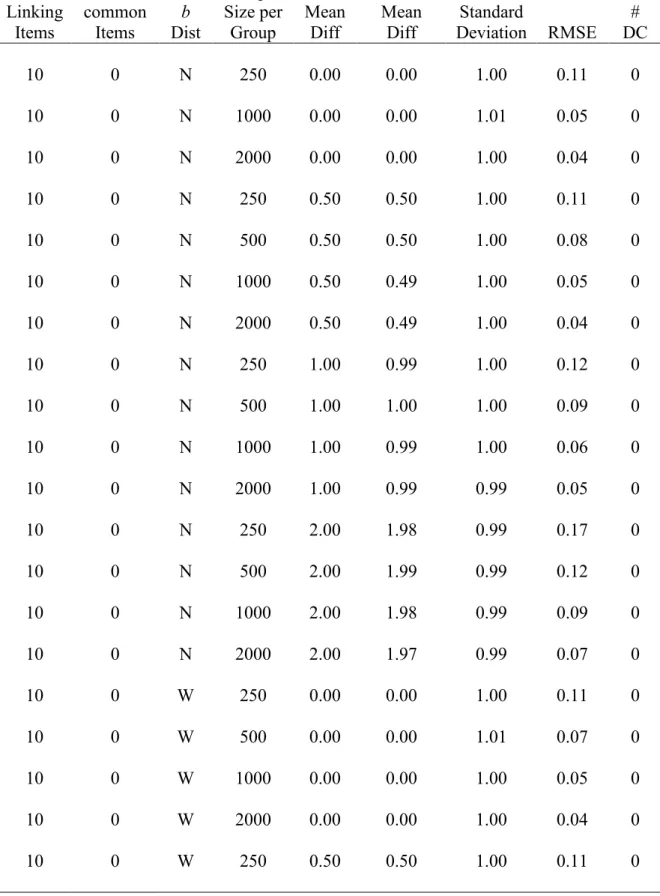
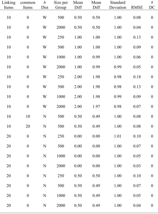
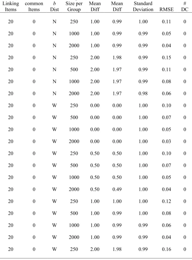
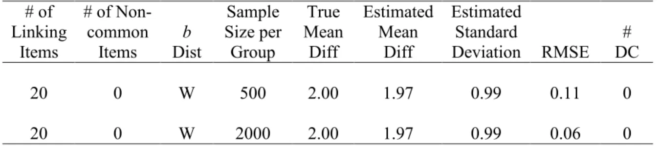
Table A1

Estimated mean differences and RMSE

# of Linking

Items

# of Non-common Items b Dist Sample Size per Group True Mean Diff Estimated Mean Diff Estimated Standard Deviation RMSE # DC

1 10 N 500 0.50 0.46 0.97 0.17 0

1 20 N 500 0.50 0.44 0.96 0.18 0

5 0 N 250 0.00 0.00 1.02 0.12 0

5 0 N 500 0.00 0.00 1.01 0.08 0

5 0 N 1000 0.00 0.00 1.01 0.06 0

5 0 N 2000 0.00 0.00 1.01 0.04 0

5 0 N 250 0.50 0.50 1.01 0.13 0

5 0 N 500 0.50 0.49 1.00 0.09 0

5 0 N 1000 0.50 0.50 1.00 0.06 0

5 0 N 2000 0.50 0.49 1.00 0.04 0

5 0 N 250 1.00 1.00 1.00 0.15 0

5 0 N 500 1.00 0.99 1.00 0.10 0

5 0 N 1000 1.00 0.99 0.99 0.07 0

5 0 N 2000 1.00 0.99 0.99 0.05 0

5 0 N 250 2.00 1.96 0.97 0.21 0

5 0 N 500 2.00 1.97 0.98 0.15 0

5 0 N 1000 2.00 1.96 0.97 0.11 0

5 0 N 2000 2.00 1.96 0.97 0.09 0

(76)

Table A1: Estimated mean differences and RMSE (continued) # of

Linking Items

5 0 N 500 3.00 2.91 0.96 0.27 0

5 0 N 1000 3.00 2.90 0.95 0.21 0

5 0 N 2000 3.00 2.89 0.95 0.17 0

5 0 N 250 4.00 3.59 0.84 0.67 11

5 0 N 500 4.00 3.66 0.86 0.52 2

5 0 N 1000 4.00 3.66 0.87 0.47 0

5 0 N 2000 4.00 3.67 0.87 0.43 0

5 0 W 250 0.00 -0.01 1.02 0.12 0

5 0 W 500 0.00 0.00 1.00 0.08 0

5 0 W 1000 0.00 0.00 1.00 0.06 0

5 0 W 2000 0.00 0.00 1.00 0.04 0

5 0 W 250 0.50 0.50 1.01 0.13 0

5 0 W 500 0.50 0.50 1.00 0.09 0

5 0 W 1000 0.50 0.50 1.00 0.06 0

5 0 W 2000 0.50 0.50 1.00 0.04 0

5 0 W 250 1.00 1.00 1.00 0.16 0

5 0 W 500 1.00 1.00 0.99 0.11 0

5 0 W 1000 1.00 0.99 0.99 0.08 0

5 0 W 2000 1.00 0.99 0.99 0.06 0

(77)

Linking Items

5 0 W 500 2.00 1.96 0.97 0.17 0

5 0 W 2000 2.00 1.96 0.97 0.10 0

5 0 W 250 3.00 2.86 0.92 0.40 0

5 0 W 500 3.00 2.88 0.93 0.30 0

5 0 W 1000 3.00 2.87 0.93 0.24 0

5 0 W 2000 3.00 2.86 0.93 0.21 0

5 0 W 250 4.00 3.38 0.75 0.88 45

5 0 W 500 4.00 3.45 0.77 0.75 22

5 0 W 1000 4.00 3.41 0.78 0.69 8

5 0 W 2000 4.00 3.51 0.79 0.62 5

5 10 N 500 0.50 0.49 0.99 0.08 0

5 10 N 250 3.00 2.84 0.93 0.42 0

5 10 N 500 3.00 2.85 0.93 0.27 0

5 10 N 1000 3.00 2.84 0.93 0.22 0

5 10 N 2000 3.00 2.84 0.93 0.19 0

5 10 N 250 4.00 2.73 0.63 1.67 0

5 10 N 500 4.00 3.24 0.75 0.98 0

5 10 N 1000 4.00 3.35 0.77 0.75 0

5 10 N 2000 4.00 3.40 0.79 0.67 0

(78)

Linking Items

10 0 N 250 0.00 0.00 1.00 0.11 0

10 0 N 1000 0.00 0.00 1.01 0.05 0

10 0 N 2000 0.00 0.00 1.00 0.04 0

10 0 N 250 0.50 0.50 1.00 0.11 0

10 0 N 500 0.50 0.50 1.00 0.08 0

10 0 N 1000 0.50 0.49 1.00 0.05 0

10 0 N 2000 0.50 0.49 1.00 0.04 0

10 0 N 250 1.00 0.99 1.00 0.12 0

10 0 N 500 1.00 1.00 1.00 0.09 0

10 0 N 1000 1.00 0.99 1.00 0.06 0

10 0 N 2000 1.00 0.99 0.99 0.05 0

10 0 N 250 2.00 1.98 0.99 0.17 0

10 0 N 500 2.00 1.99 0.99 0.12 0

10 0 N 1000 2.00 1.98 0.99 0.09 0

10 0 N 2000 2.00 1.97 0.99 0.07 0

10 0 W 250 0.00 0.00 1.00 0.11 0

10 0 W 500 0.00 0.00 1.01 0.07 0

10 0 W 1000 0.00 0.00 1.00 0.05 0

10 0 W 2000 0.00 0.00 1.00 0.04 0

(79)

Linking Items

10 0 W 500 0.50 0.50 1.00 0.08 0

10 0 W 2000 0.50 0.50 1.00 0.04 0

10 0 W 250 1.00 1.00 1.00 0.13 0

10 0 W 500 1.00 1.00 1.00 0.09 0

10 0 W 1000 1.00 0.99 1.00 0.06 0

10 0 W 2000 1.00 0.99 0.99 0.05 0

10 0 W 250 2.00 1.98 0.98 0.18 0

10 0 W 500 2.00 1.98 0.98 0.13 0

10 0 W 1000 2.00 1.98 0.99 0.09 0

10 0 W 2000 2.00 1.97 0.98 0.07 0

10 10 N 500 0.50 0.49 1.00 0.08 0

10 20 N 500 0.50 0.49 1.00 0.08 0

20 0 N 250 0.00 0.00 1.01 0.10 0

20 0 N 500 0.00 0.00 1.00 0.07 0

20 0 N 1000 0.00 0.00 1.00 0.05 0

20 0 N 2000 0.00 0.00 1.00 0.03 0

20 0 N 250 0.50 0.50 1.00 0.10 0

20 0 N 500 0.50 0.49 1.00 0.07 0

20 0 N 1000 0.50 0.49 1.00 0.05 0

(80)

Linking Items

20 0 N 250 1.00 0.99 1.00 0.11 0

20 0 N 1000 1.00 0.99 0.99 0.05 0

20 0 N 2000 1.00 0.99 0.99 0.04 0

20 0 N 250 2.00 1.98 0.99 0.15 0

20 0 N 500 2.00 1.97 0.99 0.11 0

20 0 N 1000 2.00 1.97 0.99 0.08 0

20 0 N 2000 2.00 1.97 0.98 0.06 0

20 0 W 250 0.00 0.00 1.00 0.10 0

20 0 W 500 0.00 0.00 1.00 0.07 0

20 0 W 1000 0.00 0.00 1.00 0.05 0

20 0 W 2000 0.00 0.00 1.00 0.03 0

20 0 W 250 0.50 0.50 1.00 0.10 0

20 0 W 500 0.50 0.50 1.00 0.07 0

20 0 W 1000 0.50 0.50 1.00 0.05 0

20 0 W 2000 0.50 0.49 1.00 0.04 0

20 0 W 250 1.00 1.00 1.00 0.12 0

20 0 W 500 1.00 0.99 1.00 0.08 0

20 0 W 1000 1.00 0.99 0.99 0.06 0

20 0 W 2000 1.00 0.99 0.99 0.04 0

(81)

Linking Items

20 0 W 500 2.00 1.97 0.99 0.11 0

20 0 W 2000 2.00 1.97 0.99 0.06 0

Note. A N (narrow) bdistribution refers to a uniform distribution of b’s drawn from 0.5 standard deviations below the lower group mean to 0.5 standard deviations above the higher group mean. A W (wide) bdistribution refers to a uniform distribution of b’s drawn from 1.5 standard deviations below the lower group mean to 1.5 standard deviations above the higher group mean. The true and estimated mean differences are in standard deviation units. The estimated mean difference and estimated standard deviation are the means of 1,000

(82)

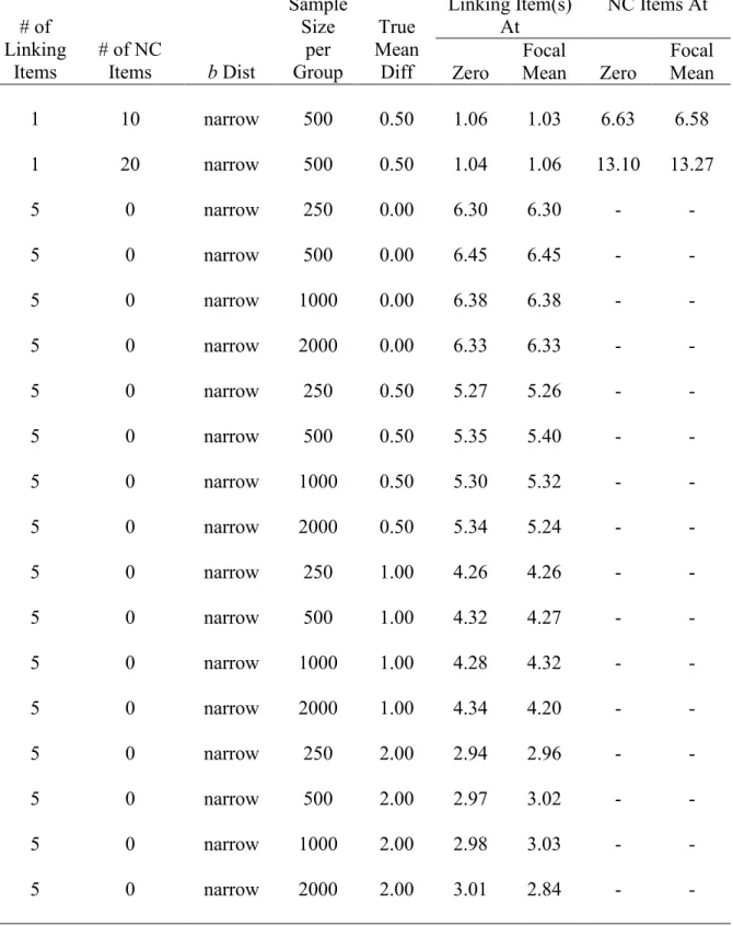
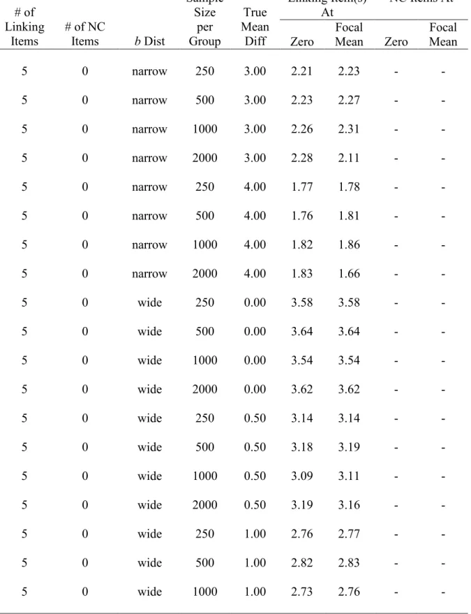
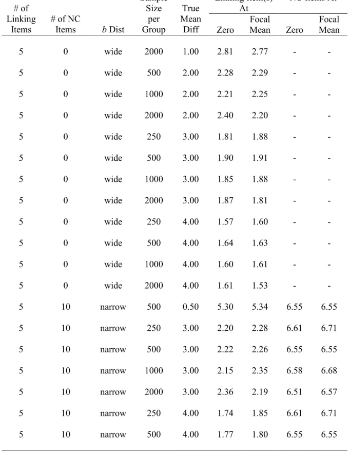
Table A2 Information Information in Linking Item(s) At Information in NC Items At # of

Linking

Items # of NC Items bDist

Sample Size per Group True Mean

Diff Zero

Focal

Mean Zero Focal Mean

1 10 narrow 500 0.50 1.06 1.03 6.63 6.58

1 20 narrow 500 0.50 1.04 1.06 13.10 13.27

5 0 narrow 250 0.00 6.30 6.30 - -

5 0 narrow 500 0.00 6.45 6.45 - -

5 0 narrow 1000 0.00 6.38 6.38 - -

5 0 narrow 2000 0.00 6.33 6.33 - -

5 0 narrow 250 0.50 5.27 5.26 - -

5 0 narrow 500 0.50 5.35 5.40 - -

5 0 narrow 1000 0.50 5.30 5.32 - -

5 0 narrow 2000 0.50 5.34 5.24 - -

5 0 narrow 250 1.00 4.26 4.26 - -

5 0 narrow 500 1.00 4.32 4.27 - -

5 0 narrow 1000 1.00 4.28 4.32 - -

5 0 narrow 2000 1.00 4.34 4.20 - -

5 0 narrow 250 2.00 2.94 2.96 - -

5 0 narrow 500 2.00 2.97 3.02 - -

5 0 narrow 1000 2.00 2.98 3.03 - -

(83)

Table A2: Information (continued)

Information in Linking Item(s)

At

Information in NC Items At # of

Linking Items

# of NC

Items bDist

Diff Zero

Focal

5 0 narrow 250 3.00 2.21 2.23 - -

5 0 narrow 500 3.00 2.23 2.27 - -

5 0 narrow 1000 3.00 2.26 2.31 - -

5 0 narrow 2000 3.00 2.28 2.11 - -

5 0 narrow 250 4.00 1.77 1.78 - -

5 0 narrow 500 4.00 1.76 1.81 - -

5 0 narrow 1000 4.00 1.82 1.86 - -

5 0 narrow 2000 4.00 1.83 1.66 - -

5 0 wide 250 0.00 3.58 3.58 - -

5 0 wide 500 0.00 3.64 3.64 - -

5 0 wide 1000 0.00 3.54 3.54 - -

5 0 wide 2000 0.00 3.62 3.62 - -

5 0 wide 250 0.50 3.14 3.14 - -

5 0 wide 500 0.50 3.18 3.19 - -

5 0 wide 1000 0.50 3.09 3.11 - -

5 0 wide 2000 0.50 3.19 3.16 - -

5 0 wide 250 1.00 2.76 2.77 - -

5 0 wide 500 1.00 2.82 2.83 - -

(84)

At

Linking Items

# of NC

Items bDist

Diff Zero

Focal

5 0 wide 2000 1.00 2.81 2.77 -

-5 0 wide 500 2.00 2.28 2.29 - -

5 0 wide 1000 2.00 2.21 2.25 - -

5 0 wide 2000 2.00 2.40 2.20 - -

5 0 wide 250 3.00 1.81 1.88 - -

5 0 wide 500 3.00 1.90 1.91 - -

5 0 wide 1000 3.00 1.85 1.88 - -

5 0 wide 2000 3.00 1.87 1.81 - -

5 0 wide 250 4.00 1.57 1.60 - -

5 0 wide 500 4.00 1.64 1.63 - -

5 0 wide 1000 4.00 1.60 1.61 - -

5 0 wide 2000 4.00 1.61 1.53 - -

5 10 narrow 500 0.50 5.30 5.34 6.55 6.55

5 10 narrow 250 3.00 2.20 2.28 6.61 6.71

5 10 narrow 500 3.00 2.22 2.26 6.55 6.55

5 10 narrow 1000 3.00 2.15 2.35 6.58 6.68

5 10 narrow 2000 3.00 2.36 2.19 6.51 6.57

5 10 narrow 250 4.00 1.74 1.85 6.61 6.71

(85)

At

Linking Items

# of NC

Items bDist

Diff Zero

Focal

5 10 narrow 1000 4.00 1.73 1.89 6.58 6.68

5 20 narrow 500 0.50 5.36 5.34 13.28 13.02

10 0 narrow 250 0.00 12.70 12.70 - -

10 0 narrow 500 0.00 12.78 12.78 - -

10 0 narrow 1000 0.00 12.78 12.78 - -

10 0 narrow 2000 0.00 12.69 12.69 - -

10 0 narrow 250 0.50 10.65 10.56 - -

10 0 narrow 500 0.50 10.63 10.69 - -

10 0 narrow 1000 0.50 10.67 10.65 - -

10 0 narrow 2000 0.50 10.57 10.61 - -

10 0 narrow 250 1.00 8.65 8.51 - -

10 0 narrow 500 1.00 8.55 8.64 - -

10 0 narrow 1000 1.00 8.61 8.59 - -

10 0 narrow 2000 1.00 8.52 8.59 - -

10 0 narrow 250 2.00 6.00 5.86 - -

10 0 narrow 500 2.00 5.88 5.96 - -

10 0 narrow 1000 2.00 5.92 5.93 - -

10 0 narrow 2000 2.00 5.88 5.94 - -

(86)

At

Linking Items

# of NC

Items bDist

Diff Zero

Focal

10 0 wide 500 0.00 7.28 7.28 -

-10 0 wide 2000 0.00 7.17 7.17 - -

10 0 wide 250 0.50 6.30 6.26 - -

10 0 wide 500 0.50 6.34 6.39 - -

10 0 wide 1000 0.50 6.35 6.30 - -

10 0 wide 2000 0.50 6.27 6.29 - -

10 0 wide 250 1.00 5.59 5.55 - -

10 0 wide 500 1.00 5.55 5.64 - -

10 0 wide 1000 1.00 5.61 5.54 - -

10 0 wide 2000 1.00 5.53 5.57 - -

10 0 wide 250 2.00 4.55 4.51 - -

10 0 wide 500 2.00 4.42 4.51 - -

10 0 wide 1000 2.00 4.50 4.45 - -

10 0 wide 2000 2.00 4.44 4.52 - -

10 10 narrow 500 0.50 10.49 10.58 6.77 6.62

10 20 narrow 500 0.50 10.65 10.67 13.00 13.08

20 0 narrow 250 0.00 25.29 25.29 - -

20 0 narrow 500 0.00 25.30 25.30 - -

(87)

At

Linking Items

# of NC

Items bDist

Diff Zero

Focal

20 0 narrow 2000 0.00 25.63 25.63 -

-20 0 narrow 500 0.50 21.14 21.09 - -

20 0 narrow 1000 0.50 21.33 21.24 - -

20 0 narrow 2000 0.50 21.30 21.49 - -

20 0 narrow 250 1.00 17.05 17.03 - -

20 0 narrow 500 1.00 17.09 17.02 - -

20 0 narrow 1000 1.00 17.23 17.12 - -

20 0 narrow 2000 1.00 17.10 17.39 - -

20 0 narrow 250 2.00 11.80 11.80 - -

20 0 narrow 500 2.00 11.81 11.73 - -

20 0 narrow 1000 2.00 11.88 11.81 - -

20 0 narrow 2000 2.00 11.66 12.01 - -

20 0 wide 250 0.00 14.31 14.31 - -

20 0 wide 500 0.00 14.36 14.36 - -

20 0 wide 1000 0.00 14.44 14.44 - -

20 0 wide 2000 0.00 14.60 14.60 - -

20 0 wide 250 0.50 12.55 12.50 - -

20 0 wide 500 0.50 12.59 12.57 - -