IMPROVEMENTS TO REAL TIME AEROSOL ANALYSIS USING AMBIENT SAMPLING/IONIZATION MASS SPECTROMETRY
Kenneth Dakota Swanson
A dissertation submitted to the faculty at the University of North Carolina at Chapel Hill in partial fulfillment of the requirements for the degree of Doctor of Philosophy in the
Department of Chemistry (Analytical) in the School of Arts and Sciences.
Chapel Hill 2018
Approved by:
James W. Jorgenson Gary L. Glish
© 2018
ABSTRACT
Kenneth Dakota Swanson: Improvements to Real Time Aerosol Analysis using Ambient Sampling/Ionization Mass Spectrometry
(Under the direction of Gary L. Glish)
Ambient ionization is a family of techniques that requires very few or no sample preparation steps and has become an important area of research in analytical applications using mass spectrometry. Extractive electrospray ionization (EESI) is an ambient
ionization technique that allows real-time sampling of organic aerosols. Similar to electrospray ionization, the composition of the electrospray solvent used in extractive electrospray ionization can easily be altered to change the chemistry of ionization. A novel EESI source design is presented to improve the reproducibility of the interactions occurring in EESI. This design uses three concentric capillaries to deliver solvent, sample and
nebulizing gas. Coaxial EESI was found to improve the inter-experiment variation by a factor of four and intra-run relative standard deviation by a factor of 2.4. Unlike most standard EESI designs, the device has the form factor of a standard electrospray (ESI) emitter and can be used without any further instrument modifications. A simple design for an open port sampling interface coupled to electrospray ionization (OPSI-ESI) is also presented as a novel approach for the analysis of aerosols. The design uses minimal
ACKNOWLEDGEMENTS
I would like to begin by thanking my advisor, Professor Gary Glish, for taking in a student who loved building with LEGOs and training him to use that creativity for science. Gary, your infectious and limitless curiosity has provided me opportunities to explore chemistry in ways no other advisor could. I will be forever grateful and inspired by your dedication to cultivate well-rounded scientists by focusing on the quality of the science rather than the quantity of results.
To the current and former members of the Glish Group, thank you for being a constant source of support, critique, and humor. You have provided a safe space for the exploration of both good and bad ideas and those collective successes and failures have made me a better scientist. I would like to particularly recognize Matt for taking the time to write and continually modify programs to make data workup easier, and for pushing me, perhaps harder than anyone else, to strive for reproducibility over settling for interesting results. Some of the work in this dissertation was completed with the aid of some hard-working undergrads. Anne, Brandon, and Katherine, thank you for following my whims and striving to produce quality data. I am also very appreciative of the graduate students who aided me in editing this dissertation (Matt, James, Nick, Paul, Tavleen, Tiffany, and Nathan).
Mom, you have always told me I can do anything I set my mind to, and I foolishly believed you. Your faith in me has propelled me to where I am today. To my brother, Curt, you and Chenoa have provided me with an inexhaustible supply of love and support. Thank you for taking me into your family and always ensuring I had everything I needed to succeed. To Dan and the men of Glee Club, thank you for giving me the opportunity to sing with you. By deeming me a tenor, you challenged me to step outside of my comfort zone and I am a far better person for it. Jerome, thank you for befriending me on my first day, for
challenging me with fun chemistry problems, and for showing me it is possible to balance a career in chemistry and a passion for music.
Finally, Brittni, whose daily encouragement was my sustaining force throughout my graduate career, words cannot express how much I love and appreciate you. Your warm smile makes each day, the good and the bad, worthwhile.
i carry your heart (i carry it in my heart)
TABLE OF CONTENTS
LIST OF TABLES ... xi
LIST OF FIGURES ... xii
LIST OF ABBREVIATIONS AND SYMBOLS ... xviii
CHAPTER 1: INTRODUCTION TO AEROSOL ANALYSIS BY AMBIENT IONIZATION MASS SPECTROMETRY ... 1
1.1 Introduction to Aerosol Particle Analysis ... 1
1.2 Analysis of the Chemical Composition of an Aerosol ... 2
1.3 Mass Spectrometry ... 4
1.4 Ambient Ionization Mass Spectrometry ... 5
1.5 Summary... 6
REFERENCES ... 8
CHAPTER 2: EXPERIMENTAL METHODS AND MATERIALS ... 12
2.1 Materials ... 12
2.2 Aerosol Generation ... 13
2.2.1 Constant Output Atomizer (COA)... 13
2.2.2 Pyroprobe ... 19
2.4 Mass Spectrometry ... 30
2.5 Ionization and Sampling ... 31
2.5.1 Electrospray Ionization ... 31
2.5.2 Extractive Electrospray Ionization (EESI) ... 33
2.5.3 Coaxial Extractive Electrospray Ionization (Coaxial EESI) ... 36
2.5.4 Open Port Sampling (OPSI) ... 36
REFERENCES ... 38
CHAPTER 3: EXTRACTIVE ELECTROSPRAY IONIZATION... 40
3.1. Introduction ... 40
3.2. Metal Cationization Extractive Electrospray Ionization Mass Spectrometry ... 41
3.2.1. Introduction to Metal Cationization EESI... 41
3.2.2. Unique Experimental Details ... 42
3.2.3. Metal Cationization EESI of Levoglucosan ... 44
3.2.4. Metal Cationization of Other Compounds Containing Multiple Oxygens ... 47
3.2.5. Tandem Mass Spectrometry of Metal Cationized Compounds ... 50
3.2.6. Conclusions ... 54
3.3. Metal Cationization during Pyrolysis of Cellulose ... 54
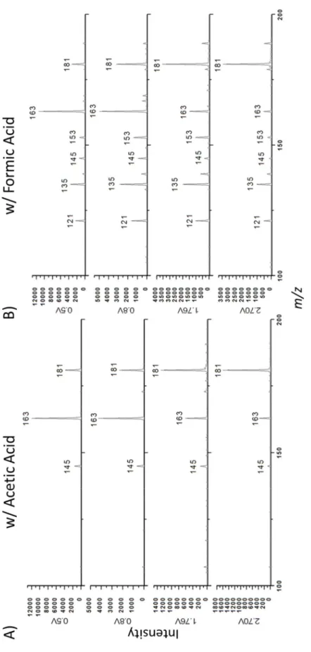
3.4. Influence of Acid Additive on EESI ... 56
3.5. Summary and Conclusions ... 65
CHAPTER 4: COAXIAL EXTRACTIVE ELECTROSPRAY IONIZATION ... 72
4.1. Introduction ... 72
4.2. Using the Aerosol-gas Flow as the Nebulization Gas ... 73
4.3. Coaxial EESI... 75
4.3.1. Design and Fabrication of a Coaxial EESI source ... 79
4.3.2. Comparison of Coaxial EESI to Standard EESI ... 84
4.4. Thermo-coaxial EESI ... 88
4.5. Solvent Composition ... 98
4.6. Port Switching ... 102
4.7. Effect on the Chemistry of Ion Formation ... 104
4.7.1. Analysis of Aerosolized Proteins by EESI ... 104
4.7.2. Analysis of Aerosolized Small Molecules using EESI ... 110
4.8. Summary and Conclusions ... 113
REFERENCES ... 117
CHAPTER 5: OPEN PORT SAMPLING INTERFACE - ELECTROSPRAY IONIZATION ... 119
5.1. Introduction ... 119
5.2. Open Port Sampling Interface coupled to Electrospray Ionization ... 120
5.2.1. Design and Operation of OPSI-ESI... 120
5.2.2. Measurement of Aspiration Rate ... 124
5.2.4. Comparison to Standard EESI ... 129
5.3. Improvements on the OPSI-ESI design for Aerosol Analysis ... 131
5.4. Solvent Composition ... 135
5.5. Summary and Conclusions ... 140
REFERENCES ... 142
CHAPTER 6: SUMMARY AND FUTURE DIRECTIONS ... 144
6.1. General Summary ... 144
6.2. Chapter Summaries ... 144
6.2.1. Chapter 3: Extractive Electrospray Ionization ... 144
6.2.2. Chapter 4: Coaxial Extractive Electrospray Ionization ... 145
6.2.3. Chapter 5: Open Port Sampling Interface – Electrospray Ionization ... 145
6.3. Future Directions ... 146
6.3.1. Quantification of Compounds in an Aerosol using OPSI-ESI ... 146
6.3.2. Structural Investigation of Compounds in Aerosol by Water Adduction ... 148
6.3.3. Separations coupled to OPSI-ESI for Complex Aerosol Analysis ... 152
LIST OF TABLES
Table 3.1. Product ion mass and neutral loss data for MS/MS of protonated, lithiated and silver-cationized levoglucosan and glucose as shown in Figure 3.6. Sodium and potassium
cationization do not produce product ions. ... 53 Table 3.2. Description of the acid sources used to investigate the acetic
acid contaminant. ... 63 Table 4.1. Tuning parameters for the comparing standard and coaxial
EESI in the analysis of oleic acid aerosol using a Bruker
HCTultra ion trap mass spectrometer. Differences between the
two configurations are bolded. ... 77 Table 4.2. Tuning parameters for the comparing standard and coaxial
EESI in the analysis of aerosolized pyrolysis products of cellulose using a Bruker Esquire 3000 ion trap mass
spectrometer. Differences between the two configurations are
LIST OF FIGURES Figure 2.1. Schematic of the constant output atomizer system
demonstrating atomization and flows. ... 14 Figure 2.2. A) AutoCAD drawing of a cap to fit a 150 mL specimen vial.
B) 3D printed caps attached to a 20 mL scintillation vial and
150 mL specimen vial. ... 16 Figure 2.3. COA with 3D printed cap on 20 mL scintillation vial in
operation. ... 18 Figure 2.4. Results from the Optimization of COA parameters. a) Size
distribution of the aerosol particles as it relates to aerosol concentration. b) Comparison of COA pressure and dilution flow rates in terms of aerosol concentration. Particle statistics shown include c) mean diameter, d) geometric mean diameter, e) median diameter, and f) mode diameter as a function of both COA
pressure and dilution flow rate... 20 Figure 2.5. Picture of the Pyroprobe model 5250 with labeled components. ... 21 Figure 2.6. Schematic of the valve operation in the Pyroprobe model
5250 with arrows indicating the direction of aerosol/gas flow. ... 23 Figure 2.7. Schematic of the manufacturer suggested mode of operation
of the Pyroprobe model 5250... 26 Figure 2.8. Time-resolved pyrolysis profiles of cellulose at varying
temperatures. ... 28 Figure 2.9. Mass spectra of cellulose pyrolysis at varying temperatures. ... 28 Figure 2.10. Time-resolved pyrolysis profiles of cellulose at varying
temperature ramp rates. ... 29 Figure 2.11. Schematic of an ESI nebulizer. ... 32 Figure 2.12. Schematic of EESI setup. ... 34 Figure 2.13. Picture of the Esquire 3000 Plus mass spectrometer
A) with the source housing intact and B) with the source
housing removed. ... 34 Figure 2.14. Picture demonstrating the arrangement of EESI in the
Figure 3.2. Comparison of concentration profiles of both [M+Li]+ and [M+Na]+ for levoglucosan by EESI. Both metals reached an
optimal intensity between 5 and 10 mM. ... 46 Figure 3.3. Comparison of [M+Li]+ and [M+Na]+ for levoglucosan from
EESI in a mixture of the two metals. Total metal concentration
was 5 mM. ... 48 Figure 3.4. Comparison of intensities resulting from cationization of
different analytes. All values were normalized to the observed ion intensity of the protonated species in the absence of added metal salt. The ratio for [M+Ag]+ is representative of the sum
of the ion intensities of both isotopes. ... 49 Figure 3.5. CID MS/MS spectra of (a) [levoglucosan+H]+, (b)
[levoglucosan+Li]+, (c) [levoglusocan+107Ag]+, (d) [glucose+H]+,
(e) [glucose+Li]+, and (f) [glucose+107Ag]+. ... 51 Figure 3.6. Full scan mass spectra of EESI of pyrolyzed ethyl cellulose
with metal salt additives. ... 55 Figure 3.7. Mass spectra of the solvent blanks using acetic acid and
formic acid as additives. ... 57 Figure 3.8. CID MS/MS spectra at varying fragmentation voltage
settings of the solvent blanks using A) acetic acid and
B) formic acid. ... 59 Figure 3.9. Bar graph of the unreactive fraction from m/z 163 observed
in the analysis of aerosolized levoglucosan using acetic acid and
formic acid as additives. ... 61 Figure 3.10. Analysis of different acid sources to observe the A)
unreactive fraction and B) intensity of m/z 163. A description
of the acid labels are given in Table 3.2. ... 64 Figure 3.11. High resolution mass spectra of the solvent blanks
containing both formic acid and acetic acid as an additive. ... 66 Figure 4.1. Mass spectra of deprotonated oleic acid ([M-H]-) using
different ionization sources. ... 74 Figure 4.2. Diagram of standard EESI. ... 76 Figure 4.3. Diagram of coaxial EESI. Solvent (blue) flows down a center
capillary surrounded by a sheath of nebulizing gas (green). Aerosol (red) flows through the outer capillary and interacts with the solvent and nebulizing gas at the tip of the emitter
Figure 4.4. (A) Assembled coaxial EESI device measuring 136 mm in length with a maximum radius of 28 mm. (B) Explosion view of the device with all pieces labeled. All pieces are assembled along
the axis shown. ... 81 Figure 4.5. (a) Fabricated coaxial EESI device measuring 136 mm in
length. (b) Zoomed image of the tip of the device showing the three concentric capillaries. (c) Zoomed image of the tip of the device to illustrate the distance each capillary extends from the
device. ... 83 Figure 4.6. Comparison between standard (red) and coaxial (blue) EESI
for the study of deprotonated oleic acid aerosol ([M-H]-) from oleic acid aerosol. The left pane is the absolute intensity of each
configuration (n=9) after disassembly and reassembly of the configuration. The center pane is a representative trace of the absolute intensity as a function of time for each configuration. The right pane is the average (n=9) of the intra-run relative
standard deviations for each trace as a function of time. ... 85 Figure 4.7. Comparison between standard (top) and coaxial (bottom)
EESI of the spectra obtained from EESI of the aerosol generated
from the pyrolysis of cellulose. ... 87 Figure 4.8. Comparison of the total ion chronogram between standard
(red) and coaxial (blue) EESI in the study of the aerosol generated from the pyrolysis of cellulose over the course of a pyrolysis
experiment. The temperature program (green) is also shown
corresponding to the green axis. ... 87 Figure 4.9. Picture showing coaxial EESI insulated from the clamp by
a 3D printed collar (brown). ... 90 Figure 4.10.Mass spectrum of deprotonated oleic acid ([M-H]-) analyzed
by thermo-coaxial EESI. The inset chronogram shows the signal
response as aerosol is introduced to the source... 92 Figure 4.11. Pictures showing A) thermo-coaxial EESI in operation and
B) standard EESI in operation on the Thermo Scientific
LTQ-FTICR mass spectrometer. ... 92 Figure 4.12. Mass spectra comparing standard and thermo-coaxial
EESI using the LTQ mass analyzer. ... 94 Figure 4.13. Mass spectra comparing standard and thermo-coaxial
Figure 4.14. Chronograms of three replicate runs tracing m/z 185 during the analysis of the aerosol generated from the pyrolysis
of cellulose using A) standard EESI and B) thermo-coaxial EESI. ... 96 Figure 4.15. Accurate mass spectra of m/z 163 using the FT-ICR shown
as A) single spectrum and B) time-resolved spectrum. ... 97 Figure 4.16. Mass spectra of the aerosol generated from the pyrolysis
of cellulose ionized by coaxial EESI using different solvent
compositions. ... 99 Figure 4.17. Histogram of peaks observed in the analysis of the aerosol
generated from the pyrolysis of cellulose using coaxial EESI with different solvent compositions. The inset bar graph shows
the total number of peaks observed for each solvent composition. ... 101 Figure 4.18. Pictures of the coaxial EESI device A) originally, B) after
reinforcement, and C) an AutoCAD drawing of the plastic support. ... 103 Figure 4.19. A chronogram of the analysis of the aerosol generated
from the pyrolysis of cellulose using coaxial EESI in different
modes of operation and at different flow rates. ... 105 Figure 4.20. Aerosol size distribution of a blank aerosol and an aerosol
containing lysozyme. ... 107 Figure 4.21. Analysis of lysozyme using different ionization techniques. ... 108 Figure 4.22. Analysis of ubiquitin using different ionization techniques. ... 109 Figure 4.23. Mass spectra of lysozyme from an aerosol analyzed by
standard EESI with and without the use of an electrospray solvent. ... 111 Figure 4.24. Mass spectra of lysozyme from an aerosol analyzed by
coaxial EESI with and without the use of an electrospray solvent. ... 111 Figure 4.25. Comparison of the response of lithiated levoglucosan,
m/z 169 to the addition of lithium to the electrospray solvent
in both standard and coaxial EESI. ... 112 Figure 4.26. Mass spectra of the aerosol generated from the pyrolysis
of cellulose analyzed by coaxial EESI with and without the use
of an electrospray solvent. ... 114 Figure 5.1. Schematic of open port sampling interface – electrospray
ionization (OPSI-ESI) A) without aerosol introduction and B) with aerosol
introduction. ... 121 Figure 5.2. Comparison of OPSI-ESI emitter and a standard ESI
Figure 5.3. Plot of gas velocity versus aspiration rate through the inner
capillary (N=5). ... 125 Figure 5.4. Figure showing the response of OPSI-ESI to an aerosol of
nicotine at 159 m s-1(blue), 247 m s-1(orange), 326 m s-1 (grey), and 405 m s-1 (purple) gas velocities. The red trace indicates whether aerosol was directed toward the OPSI-ESI interface
(ON) or away from the OPSI-ESI interface (OFF). ... 127 Figure 5.5. (a) Mass spectra obtained using OPSI-ESI for the analysis
of pyrolyzed cellulose, EESI for the analysis of pyrolyzed cellulose, OPSI-ESI for the analysis of pyrolyzed lignin extracted from tobacco, and OPSI-ESI for the analysis of pyrolyzed hemicellulose extracted from tobacco. A comparison of the total ion count across the mass range 15 to 250 m/z for
both OPSI-ESI and EESI of pyrolyzed cellulose (N=3) is shown in (b). ... 130 Figure 5.6. Picture of the modular OPSI-ESI device A) alone and B)
attached to a Bruker ESI emitter. ... 133 Figure 5.7. Plot showing the relationship of nebulization gas to
aspiration rate for each the standard and modular OPSI-ESI
devices. ... 133 Figure 5.8. Picture of the modular OPSI-ESI device on a Thermo
Scientific Ion Max source. ... 134 Figure 5.9. Extracted ion chronogram of caffeine, m/z 195, sampled
from an aerosol with the modular OPSI-ESI device on the Thermo Scientific Ion Max source. The orange trace indicates
the presence or absence of aerosol at the solvent interface. ... 136 Figure 5.10. Mass spectra of the aerosol generated from the pyrolysis
of cellulose ionized by OPSI-ESI using different solvent
compositions. ... 138 Figure 5.11. Histogram of peaks observed in the analysis of the aerosol
generated from the pyrolysis of cellulose using OPSI-ESI with different solvent compositions. The inset bar graph shows the
total number of peaks observed for each solvent composition. ... 139 Figure 6.1. GC-MS chromatograms of aerosol collected onto a filter
and extracted in methanol for two different methods of aerosol
generation. ... 147 Figure 6.2. Bar graph showing the reactivity of α-methylglucoside
ionized by ESI and EESI under two different dry gas flow rates. ... 149 Figure 6.3. Graph showing the relationship of unreactive fraction of
Figure 6.4. Graph showing the unreactive fraction of glucose-12C and
LIST OF ABBREVIATIONS AND SYMBOLS
3D three-dimensional
AIM aerosol instrument manager
AMS aerosol mass spectrometer
APCI atmospheric pressure chemical ionization
°C degrees Celsius
-C13 isotopically labeled with carbon-13
CID collision induced dissociation
CO carbon monoxide
COA constant output atomizer
CPC condensation particle counter
cm centimeter
Da unified atomic mass unit
DESI desorption electrospray ionization
DFT density functional theory
DIMS differential ion mobility spectrometry
DMA differential mobility analyzer
-dn isotopically labeled with n deuterium atoms EESI extractive electrospray ionization
EI electron ionization
EIC extracted ion chronogram
ESI electrospray ionization
FA formic acid
FT-ICR Fourier transform – ion cyclotron resonance
GC gas chromatography
g gram
H2O water
HESI heated electrospray ionization
HOAc acetic acid
HV high voltage
hr hour
ID inner diameter
IEM ion evaporation model
in inch
kV kilovolt
L liter
LC liquid chromatography
LPM liters per minute
LTPI low temperature plasma ionization
MeOH methanol
MS mass spectrometry
MS/MS tandem mass spectrometry
MSn n stages of mass spectrometry
m meter
m/z mass-to-charge ratio
mA milliampere
mL milliliter
mM millimolar
mm millimeter
ms millisecond
min minute
µA microampere
µL microliter
µM micromolar
µg microgram
µm micrometer
µs microsecond
n=4 number of replicates
N2 nitrogen
NL intensity of the most abundant peak
NNN n-nitrosonornicotine
NPT national pipe thread taper
nA nanoampere
nm nanometer
OD outer diameter
OPSI open port sampling interface
PILS particle-into-liquid sampler
PLA polylactic acid
ppm part-per-million
psig pounds per square inch gauge
QIT quadrupole ion trap
RSD relative standard deviation
SCFM standard cubic feet per minute
SMPS scanning mobility particle sizer
TIC total ion chronogram
UR unreactive rate
V volts
Vpp peak-to-peak voltage
v/v volume/volume percent
ZDV zero dead volume
[M+H]+ positively charged protonated analyte
CHAPTER 1: INTRODUCTION TO AEROSOL ANALYSIS BY AMBIENT IONIZATION MASS SPECTROMETRY
1.1. Introduction to Aerosol Particle Analysis
Aerosol particle analysis presents a significant analytical challenge due to variations in size, composition, and phase1. An aerosol is a system of small particles suspended in a gas. A single aerosol particle is a conglomeration of molecules that can range in diameter from a few nanometers (nm), a collection of a two or more molecules, to ten microns (m)2. The lifetimes of aerosol particles are inversely proportional to the particle size. The
Environmental Protection Agency has set regulation standards for particles less than 10
m in diameter because they can penetrate deep into the lungs3. Particular attention is given to aerosol particles 2.5 m or less in diameter due to the environmental damage of particles that can travel long distances and settle onto the ground or into water sources. Depending on the chemical composition of these particles, this settling can cause reduction of visibility, acidification of lakes and streams, depletion of nutrients in soil, and damage to forestry and farm crops4. Further, the World Health Organization estimated that exposure to airborne pollution particles results in approximately 348,000 premature deaths every year5. Unless particles are specifically produced to be of a single diameter, or monodisperse, aerosol particles are typically polydisperse in size. This is important because aerosol
assumption because the chemical composition of aerosol particles are often a function of particle size as shown in the literature6,7.
Any single aerosol particle can be heterogeneous or homogeneous depending on the phase of the particle, where the phase can be a liquid, solid, or a mixture of both. Thus, analysis of the surface of a particle may not be representative of the whole particle, especially when constituents are insoluble in a liquid droplet, forming a heterogeneous particle. This becomes important in analyses where solubility is a factor in extracting compounds from the particle.
1.2. Analysis of the Chemical Composition of an Aerosol
The analysis of the chemical composition of an aerosol is critical to many different fields, including secondary organic aerosol formation8,9, drug delivery10,11, biological warfare agents12, and biomass burning13. An analysis method can generally be grouped by two categories: amount of sample preparation and the ability to distinguish particles from one another. The amount of sample preparation required by an analysis determines whether an analysis is on-line (little or no sample preparation) or off-line (sample preparation is
required). The ability to distinguish particles from one another determines whether the aerosol is sampled in bulk (particles analyzed without respect to size), size-separated prior to analysis, or analyzed on a single-particle level.
represent the compounds present in the aerosol particles immediately after generation. Further, no information regarding particle size or composition as a function of size is obtained.
Particles may be size-separated prior to either off-line or on-line analyses, but both present significant challenges17. Any off-line analysis will suffer from the aforementioned chemical aging, reactions with surfaces, and evaporative losses. On-line analyses of size-selected particles include the use of a scanning mobility particle sizer (SMPS) system18. An SMPS system, such as a differential mobility analyzer (DMA), separates particles by first charging particles uniformly and then separating the particles using an electric field19. The trajectory of smaller particles will be easily changed in a small electric field while larger particles require a larger electric field20. Size-separated particles are usually detected using a laser system such as a condensation particle counter21. While a laser system gives
information on the distribution of sizes in an aerosol, it gives no information on the chemical composition of an aerosol.
Another method of aerosol size-separation is used prior to mass analysis in the
commercial Aerodyne Aerosol Mass Spectrometer (AMS)22–24. This system utilizes a time-of-flight particle measurement where particles are accelerated with the same kinetic energy22. The velocity of each particle is determined by its mass, thus smaller particles arrive at the electron impact (EI) ionization source of the mass spectrometer earlier than larger particles yielding a separation of particles in time. For this analysis, a fast mass analyzer is required such as a quadrupole or a time-of-flight. The information obtained in this analysis includes size distribution of the aerosol particles, but the compositional analysis is limited to
determination of compound classes rather than molecular assignment25. The EI source imparts enough internal energy to both ionize a compound and induce significant
may be determined from the fragmentation pattern if only a single species if present, but compound identification is very difficult in a complex mixture due to overlapping
fragmentation patterns. For this reason, the AMS system is ill-suited for compound identification in an aerosol. Custom-built mass spectrometers have been built for single-particle analyses, but these involve laser-induced ionization which suffers from the same drawbacks as EI where relative abundance of compound classes may be determined, but compound identification is very difficult26–29.
1.3. Mass Spectrometry
Mass spectrometry is a fast, highly selective, and sensitive analysis technique that is uniquely suited for chemical analysis of complex mixtures. For successful mass analysis of the intact molecular ions from a sample, an analyte must be converted from its native state into gaseous ions. For an aerosol, particles must be dissociated into individual molecules and ionized. EI is often used in tandem with mass analysis due to the ability to control the energy of ionization. However, it typically imparts too much internal energy for the direct analysis of complex samples leading to excessive fragmentation and convoluted spectra. These ionization techniques are typically used in conjunction with chromatographic techniques such as liquid chromatography (LC) or gas chromatography (GC) to reduce sample complexity prior to mass analysis. Unfortunately, neither LC nor GC are very amenable to on-line aerosol analysis because both techniques usually begin with a sample in the liquid phase. To use chromatographic separations with an on-line aerosol analysis, an aerosol sample would have to be put into solution and injected onto a column on a fast timescale that reduces chemical aging.
can occur, depending on the electric fields generated by the ion optics, but ESI is generally considered a soft-ionization technique. In ESI, an electric field is generated by applying a potential difference between the inlet to the mass spectrometer and a capillary containing the analyte of interest dissolved in solution32. Charge accumulates on the solution at the tip of the capillary and a Taylor cone of solution is formed from which small, highly charged droplets are ejected toward the mass spectrometer. By the ion evaporation model (IEM), a droplet desolvates until the surface charge reaches the Rayleigh limit33 and the droplet explodes into smaller droplets due to columbic repulsion of the charges. Over time, solvated ions are ejected from the charged droplet. The solvent evaporates from the solvated ion until bare analyte ions are transmitted through the mass spectrometer for mass analysis34. Similar challenges exists for ESI as for LC or GC analysis. In ESI, the sample needs to be dissolved in solution before ionization. An aerosol would have to be put into solution and electrosprayed on a fast timescale that reduces chemical aging.
1.4. Ambient Ionization Mass Spectrometry
Ambient ionization refers to a family of ionization techniques in mass spectrometry in which ionization occurs at atmospheric pressure prior to introduction of the ions into the vacuum region of the mass spectrometer35–39. Benefits of ambient ionization include minimal or no sample preparation and the ability to analyze samples from their native state in real-time39. Ambient ionization can be broadly classified into laser-based techniques, atmospheric pressure chemical ionization (APCI)-related techniques, and electrospray-based techniques40.
plate. This type of analysis allows for concentration of the aerosol for increased signal intensity; however, the technique suffers from problems similar to filter collection as discussed earlier. A particle-into-liquid sampler (PILS) has also been used to sample from aerosols resulting from biomass burning prior to electrospray ionization42. Both of these techniques require sample collection prior to analysis by mass spectrometry and are susceptible to chemical aging and evaporative losses.
Real-time ambient ionization has also been applied to aerosol particles. Low
temperature plasma ionization (LTPI) has been used to characterize organic aerosols in which the plasma from a dielectric barrier discharge intersects a stream of organic aerosol particles43,44. The most reported technique for the on-line characterization of aerosol particles is extractive electrospray ionization (EESI)45–47. EESI involves a real-time
extraction by colliding aerosol particles with the electrospray plume. This technique is one of the most versatile ionization techniques currently available for bulk aerosol analysis due to the ability to easily alter the extraction by manipulation of the electrospray solvent composition48,49. These techniques do not require significant instrument modifications as they can be used on any mass spectrometer with an atmospheric pressure interface. 1.5. Summary
The experimental methods used in subsequent chapters are provided in Chapter 2. The instrumentation used is also covered, including information about the aerosol generation systems, the electrospray ionization source, the extractive electrospray ionization source, and the mass spectrometry systems used.
The work presented in Chapter 3 involves the use of EESI to improve the sensitivity of multiple oxygen-containing compounds by using metal cations in the electrospray
solvent. Fortuitously, this also led to improved dissociation patterns upon MS/MS of two of the compounds analyzed. Some studies are presented to show the similarity in the
structures formed by EESI and ESI.
Chapter 4 discusses the drawbacks of the current EESI source and outlines a new design for a more stable source that can be used with the existing source housing. The fabrication of a coaxial EESI source is discussed and characterization of this source is presented in comparison to the existing EESI source. Solvent composition optimization for coaxial EESI is presented in the study of pyrolyzed cellulose.
REFERENCES
1. Prather, K. A., Hatch, C. D. & Grassian, V. H. Analysis of Atmospheric Aerosols. Annu. Rev. Anal. Chem. 1, 485–514 (2008).
2. Kaiser, J. Mounting Evidence Indicates Fine-Particle Pollution. Science 307, 1858– 1861 (2005).
3. Particulate Matter (PM) Basics. US Environmental Protection Agency (2016). Available at: https://www.epa.gov/pm-pollution/particulate-matter-pm-basics. 4. Health and Environmental Effects of Particulate Matter (PM). US Environmental
Protection Agency (2003). Available at: https://www.epa.gov/pm-pollution/health-and-environmental-effects-particulate-matter-pm.
5. Joint WHO / Convention Task Force on the Health Aspects of Air Pollution. Health risks of particulate matter from long-range transboundary air pollution. (2006). 6. Lundgren, D. A. Atmospheric Aerosol Composition and Concentration as a Function
of Particle Size and of Time. J. Air Pollut. Control Assoc. 20, 603–608 (1970). 7. Noble, C. A. & Prather, K. A. Real-Time Measurement of Correlated Size and
Composition Profiles of Individual Atmospheric Aerosol Particles. Envionmental Sci. Technol. 30, 2667–2680 (1996).
8. Surratt, J. D. et al. Chemical Composition of Secondary Organic Aerosol Formed from the Photooxidation of Isoprene. J. Phys. Chem. A 110, 9665–9690 (2006).
9. Krechmer, J. E. et al. Formation of Low Volatility Organic Compounds and
Secondary Organic Aerosol from Isoprene Hydroxyhydroperoxide Low-NO Oxidation. Environ. Sci. Technol. 49, 10330–10339 (2015).
10. Arunthari, V., Bruinsma, R. S., Lee, A. S. & Johnson, M. M. A Prospective,
Comparative Trial of Standard and Breath-Actuated Nebulizer: Efficacy, Safety, and Satisfaction. Respir. Care 57, 1242–1247 (2012).
11. Smith, J. H. et al. Nebulized live-attenuated influenza vaccine provides protection in ferrets at a reduced dose. Vaccine 30, 3026–3033 (2012).
12. Pazienza, M. & Britti, M. S. Use of Particle Counter System for the Optimization of Sampling, Identification and Decontamination Procedures for Biological Aerosols Dispersion in Confined Environment. J. Microb. Biochem. Technol. 06, 43–48 (2013). 13. Brito, J. et al. Ground-based aerosol characterization during the South American
Biomass Burning Analysis (SAMBBA) field experiment. Atmos. Chem. Phys. 14, 12069–12083 (2014).
15. Bateman, A. P. et al. The effect of solvent on the analysis of secondary organic aerosol using electrospray ionization mass spectrometry. Environ. Sci. Technol. 42, 7341– 7346 (2008).
16. Turpin, B. J., Saxena, P. & Andrews, E. Measuring and simulating particulate organics in the atmosphere: Problems and prospects. Atmos. Environ. 34, 2983–3013 (2000).
17. McMurry, P. A review of atmospheric aerosol measurements. Atmos. Environ. 34, 1959–1999 (2000).
18. Keady, P. B., Quant, F. R. & Sem, G. J. Differential mobility particle sizer: a new instrument for high-resolution aerosol size distribution measurement below 1 µm. TSI Q. 9, 3–11 (1983).
19. Liu, B. Y. H. & Pui, D. Y. H. Electrical neutralization of aerosols. J. Aerosol Sci. 5, 465–472 (1974).
20. Hagen, D. E. & Alofs, D. J. Linear Inversion Method to Obtain Aerosol Size
Distributions from Measurements with a Differential Mobility Analyzer. Aerosol Sci. Technol. 2, 465–475 (1983).
21. Wiedensohlet, A. et al. Intercomparison study of the size-dependent counting efficiency of 26 condensation particle counters. Aerosol Sci. Technol. 27, 224–242 (1997).
22. Canagaratna, M. R. et al. Chemical and microphysical characterization of ambient aerosols with the aerodyne aerosol mass spectrometer. Mass Spectrom. Rev. 26, 185– 222 (2007).
23. Shilling, J. E., King, S. M., Mochida, M., Worsnop, D. R. & Martin, S. T. Mass spectral evidence that small changes in composition caused by oxidative aging processes alter aerosol CCN properties. J. Phys. Chem. A 111, 3358–3368 (2007). 24. Jimenez, J. L. et al. Evolution of Organic Aerosols in the Atmosphere: A New
Framework Connecting Measurements to Models. Science (80-. ). 326, 1525–1529 (2009).
25. Zahardis, J., Geddes, S. & Petrucci, G. A. Improved Understanding of Atmospheric Organic Aerosols via Innovations in Soft Ionization Aerosol Mass Spectrometry. Anal. Chem. 83, 2409–2415 (2011).
26. Denkenberger, K. A., Moffet, R. C., Holecek, J. C., Rebotier, T. P. & Prather, K. A. Real-time, single-particle measurements of oligomers in aged ambient aerosol particles. Environ. Sci. Technol. 41, 5439–5446 (2007).
28. Hatch, L. E., Pratt, K. A., Huffman, J. A., Jimenez, J. L. & Prather, K. A. Impacts of Aerosol Aging on Laser Desorption/Ionization in Single-Particle Mass Spectrometers. Aerosol Sci. Technol. 48, 1050–1058 (2014).
29. Axson, J. L., May, N. W., Colón-Bernal, I. D., Pratt, K. A. & Ault, A. P. Lake Spray Aerosol: A Chemical Signature from Individual Ambient Particles. Environ. Sci. Technol. 50, 9835–9845 (2016).
30. Fenn, J. B. Electrospray Wings for Molecular Elephants (Nobel Lecture). Angew. Chemie Int. Ed. 42, 3871–3894 (2003).
31. Covey, T. R., Thomson, B. A. & Schneider, B. B. Atmospheric pressure ion sources. Mass Spectrom. Rev. 28, 870–897 (2009).
32. Wong, S. F., Meng, C. K. & Fenn, J. B. Multiple Charging in Electrospray Ionization of Poly(ethylene glycols). J. Phys. Chem. 92, 546–550 (1988).
33. Rayleigh, Lord. XX. On the equilibrium of liquid conducting masses charged with electricity. London, Edinburgh, Dublin Philos. Mag. J. Sci. 14, 184–186 (1882). 34. Iribarne, J. V. On the evaporation of small ions from charged droplets. J. Chem.
Phys. 64, 2287 (1976).
35. Ifa, D. R., Wu, C., Ouyang, Z. & Cooks, R. G. Desorption electrospray ionization and other ambient ionization methods: current progress and preview. Analyst 135, 669– 681 (2010).
36. Huang, M.-Z., Yuan, C.-H., Cheng, S.-C., Cho, Y.-T. & Shiea, J. Ambient Ionization Mass Spectrometry. Annu. Rev. Anal. Chem. 3, 43–65 (2010).
37. Harris, G. A., Galhena, A. S. & Fernandez, F. M. Ambient sampling/ionization mass spectrometry: Applications and current trends. Anal. Chem. 83, 4508–4538 (2011). 38. Yao, Z.-P. Characterization of proteins by ambient mass spectrometry. Mass
Spectrom. Rev. 31, 437–447 (2012).
39. Wu, C., Dill, A. L., Eberlin, L. S., Cooks, R. G. & Ifa, D. R. Mass spectrometry imaging under ambient conditions. Mass Spectrom. Rev. 32, 218–243 (2013). 40. Weston, D. J. Ambient ionization mass spectrometry: current understanding of
mechanistic theory; analytical performance and application areas. Analyst 135, 661– 668 (2010).
41. Laskin, J. et al. High-Resolution Desorption Electrospray Ionization Mass
42. Bateman, A. P., Nizkorodov, S. A., Laskin, J. & Laskin, A. High-Resolution Electrospray Ionization Mass Spectrometry Analysis of Water-Soluble Organic Aerosols Collected with a Particle into Liquid Sampler. Anal. Chem. 82, 8010–8016 (2010).
43. Spencer, S. E., Tyler, C. A., Tolocka, M. P. & Glish, G. L. Low-Temperature Plasma Ionization-Mass Spectrometry for the Analysis of Compounds in Organic Aerosol Particles. Anal. Chem. 87, 2249–2254 (2015).
44. Spencer, S. E., Santiago, B. G. & Glish, G. L. Miniature Flow-Through
Low-Temperature Plasma Ionization Source for Ambient Ionization of Gases and Aerosols. Anal. Chem. 87, 11887–11892 (2015).
45. Doezema, L. A. et al. Analysis of secondary organic aerosols in air using extractive electrospray ionization mass spectrometry (EESI-MS). RSC Adv. 2, 2930 (2012). 46. Gallimore, P. J. & Kalberer, M. Characterizing an extractive electrospray ionization
(EESI) source for the online mass spectrometry analysis of organic aerosols. Environ. Sci. Technol. 47, 7324–7331 (2013).
47. Swanson, K. D., Spencer, S. E. & Glish, G. L. Metal Cationization Extractive Electrospray Ionization Mass Spectrometry of Compounds Containing Multiple Oxygens. J. Am. Soc. Mass Spectrom. 28, 1030–1035 (2017).
48. Swanson, K. D., Worth, A. L. & Glish, G. L. A coaxial extractive electrospray ionization source. Anal. Methods 9, 4997–5002 (2017).
CHAPTER 2: EXPERIMENTAL METHODS AND MATERIALS 2.1. Materials
All solvents used for electrospray ionization and related solvent-assisted ionization processes were purchased from either Thermo Fisher Scientific (Hampton, NH) or Sigma-Aldrich Corporation (St. Louis, MO) at a purity grade of Optima® unless otherwise noted. The solvents used include water (Fisher, W7-4), acetonitrile (Fisher, A996-4), methanol (Fisher, A454-4), chloroform (Fisher, Certified ACS, C298-500), toluene (Fisher, Certified ACS, T324-500), dichloromethane (Fisher, Certified ACS, D37-500). Acid additives to the electrospray solvent include acetic acid (Fisher, A113-50) and formic acid (Fisher, A117-50). Metal salt additives to the electrospray solvent include lithium acetate dihydrate (Sigma, Reagent-grade, L6883), sodium acetate (Fisher, Certified ACS, S-210), potassium acetate (Sigma, ACS reagent, 236497), and silver trifluoroacetate (Sigma, 98%, T62405). For metal cationization studies, the analytes targeted for analysis include levoglucosan (Carbosynth, 98%, ML06636 or Sigma, 99%, 316555), syringol (Sigma, 99%, D135550), maltol (Sigma, analytical standard, 18299), D-glucose (Sigma, >99.5%, G8270), and syringaldehyde (Sigma, 98%, S7602-5G). Other small molecules analytes used oleic acid (Fluka, >99%, 75090), nicotine (Sigma, >99%, N3876), N-Nitrosonornicotine (TRC, KIT0570), caffeine, (Sigma, ReagentPlus, C0750), methyl-α-D-glucopyranoside (Carbosynth, 98%, MM03961), and methyl- β-D-glucopyranoside (Carbosynth, 98%, MM03162). Isotopically labeled standards that were used include D-glucose-13C6 (Sigma, 99%, 389374),
peptide in an aerosol, leucine enkephalin (Sigma, >95%, L9133) was used. For the analysis of protein in an aerosol, lysozyme from chicken egg white (Sigma, >90%, L6876), ubiquitin from bovine red blood cells (Sigma, BioUltra, U6253), and myoglobin from equine heart (Sigma, >90%, M1882) were prepared in predominantly methanolic solutions with 10% added water to enhance solubility. For the analysis of pyrolysis products of biomass, microcrystalline cellulose (Alfa Aesar, A17730) was used. Sample extracts of lignin and hemicellulose from tobacco were provided by R.J. Reynolds Tobacco Company (Winston-Salem, NC). Raw tobacco that was genetically engineered to have low nicotine content was also provided by R.J. Reynolds Tobacco Company.
2.2. Aerosol Generation
2.2.1. Constant Output Atomizer (COA)
Two methods of aerosol generation were employed for the characterization of the ambient sampling devices discussed in this dissertation. A constant output atomizer (Model 3076, TSI Inc., Shoreview, MN) was used to generate a polydisperse aerosol from a
by a second nitrogen flow to aid in desolvation. In some cases, the dilution tube was
removed for analysis. Particles flow out of the output port of the dilution tube to the desired sampling apparatus with an aerosol gas flow that ranged from 0.5 to 12 L/min.
The solution reservoir intended to be used with the system is a 1L plastic-coated glass bottle designed with unique threads to fit the plastic cap provided with the system. The smallest amount of solution that one can use in the solvent reservoir is determined by the length of the metal tube that extends into solution. When there is insufficient solvent to reach the metal tube, aspiration no longer occurs. In time, the solution will evaporate with continued nitrogen flow. The minimum solution volume that can be used and generate an aerosol is about 200 mL. In an effort to reduce the volume of solution required for aerosol generation, a new plastic cap was designed in AutoCAD and 3D printed. Two designs were considered for 3D printing, a cap to fit a 20 mL scintillation vial and one to fit a 150 mL specimen container as shown in Figure 2.2. The threading was matched to the unique threads of each container so that the cap could be securely twisted onto the desired
container. Three holes were printed or drilled into the caps for the pressure relief valve, the metal aspirating tube, and the solution return in recirculation mode. Each hole was printed or drilled to be slightly larger than 0.375” in diameter to accommodate NPT threads. A new metal aspirating tube was made using 0.125” stainless steel tubing, a stainless steel ultra-torr vacuum fitting (Swagelok, SS-8-UT-1-6), and appropriately sized
o-rings. The tubing was cut to extend to the bottom of the container in each case and the tubing was secured to the vacuum fitting by sliding the o-rings onto one end of the tubing and inserting the assembly into the NPT end of the vacuum fitting. The vacuum fitting was then secured to the cap by threading onto the central-most hole in the cap to allow
pressure relief valve were transplanted from the original cap as shown in Figure 2.3. Care was taken in the design process to ensure enough room for the plastic tubing that
accompanies the solvent return while keeping the holes far enough apart to avoid cracking the print material. When pressurized, the seal created by the scintillation vial threading onto the cap was not very good as methanol aerosol was observed leaking from the connection. One layer of electrical tape placed on the threads of the scintillation vial was enough to create a good seal.
For the 20 mL scintillation vial, a minimum of 5mL was necessary to form an aerosol. In this configuration, the aerosol solution disappeared at a much higher rate than expected. No single source of leakage was observed, instead the outer surface of the 3D printed cap became wet. It appears that even at high print resolution, the pores inherent to 3D printing are too large to create a sufficient seal for prolonged and reproducible aerosol generation.
The settings for the COA were studied and optimized using a scanning mobility particle sizer system (described in Section 2.3), and the results are displayed in Figure 2.4. The most crucial settings for the COA system are the pressure at the atomizer
(COA pressure) and the flow rate of the dilution flow. The COA pressure and the solvent reservoir pressure that is regulated by the pressure relief valve are different due to a pressure drop across the system. A representative size distribution of oleic acid dissolved in methanol is shown in Figure 2.4a. The aerosol is polydisperse, but normally distributed around a mean diameter of 51 nm at 5 standard cubic feet per minute (SCFM) and 30 psig COA pressure. The green markers in Figure 2.4b-f represent 3 SCFM dilution flow and the blue markers represent 5 SCFM dilution flow. No significant difference was observed when the dilution flow was changed in this study. Shown in Figure 2.4b, the total aerosol
concentration was observed to increase linearly as the COA pressure was increased. At COA pressures above 30 psig, the pressure relief valve on the solvent reservoir periodically released, which changed the pressure in the system. For this reason, no COA pressures above 30 psig were studied. Particle statistics of mean, geometric mean, median, and mode diameters at different COA pressures are shown in Figures 2.5c-f. Generally, the mean, geometric mean, and median diameters decreased as COA pressure increased, which suggests that smaller droplets are created by the larger linear velocity at the atomizer aperture. If smaller droplets are formed from the same volume, more droplets are formed. 2.2.2. Pyroprobe
to provide a surface for a solid sample to rest inside the tube while allowing some flow through the sample. A sample is then loaded into the tube ranging from 5-20 mg of material. The filled sample tube is placed into the autosampler of the Pyroprobe 5250 shown in Figure 2.5. The valve oven is held at 300 °C at all times. This oven (Figure 2.5h), keeps the bottom valve, 8-port valve and tubing warm to avoid condensation of the aerosol particles onto surfaces. The autosampler (Figure 2.5b) actuates the sample tube (Figure 2.5a) to be in line with the pyrolysis chamber (Figure 2.5e), and the sample tube is dropped onto a closed top valve (Figure 2.5c). The top valve is then actuated into an open position, causing the sample tube to drop into the chamber (Figure 2.5d) onto a closed bottom valve (Figure 2.5f). The top valve then closes, sealing the sample tube into the pyrolysis chamber. The 8-port valve (Figure 2.5i) actuates to flow pure nitrogen through the pyrolysis chamber. A current is then applied to the chamber heating coil (Figure 2.5e) to heat the pyrolysis chamber. A typical heating program for most samples included in this work is as follows. The sample is equilibrated in the chamber for 10 seconds with the heating coil at 25 °C. The sample is then heated at a rate of 10 °C/s to a temperature of 650 °C and held at that
temperature for 5 minutes. These values were typically used for analysis, but other settings were studied and the results are discussed below. At the end of the heating period, the bottom valve is actuated and the sample tube is ejected through the bottom chute (Figure 2.5g).
where there is no flow through the pyrolysis chamber. Pure nitrogen flows into the 5th port of the 8-port valve directly to the output. The plumbing in Figure 2.6 is not the
manufacturer suggested mode of operation. The instrument was modified to this mode of operation for the purpose of improved signal intensity upon sampling of the generated aerosol3. The problems created by using this mode of operation include increased clogging, instability of the sample tube, and frequent breakage of sample tubes. The clogging
observed has been attributed to two sources. The first source of clogging is due to the direction of gas flow in the pyrolysis chamber in position 1. Large sample particles and aerosol are easily blown out of the sample tube to the outlet of the top valve. The second source of clogging was condensation of particles inside the top valve and the following tubing due to a decrease in temperature. The top valve is not directly heated by the oven in the same way as the bottom valve, thus particles are more likely to settle and condense onto cooler surfaces. Clogging was frequently observed at the output of the top valve and in the tube connecting the top valve to the 8-port valve, which was only solved by flowing solvent in the opposite direction to the gas flow to dislodge the clog.
dropped out of the chamber. If the sample tube stopped falling inside either one of the valves, the valve would actuate based upon a timer and crush the sample tube. A crushed tube requires extensive cleaning of the valves and pyrolysis chamber to remove broken quartz pieces. Further, when the 8-port valve was in position 2, no sample was loaded into the probe, but no gas flowed through the chamber. Any sample material that had blown outside the tube would remain in the chamber, causing buildup of char inside the chamber which led to an ongoing need to clean the system.
These problems were not solved until the Pyroprobe was returned to manufacturer specifications as shown in Figure 2.7. In this mode, the flow of gas in the chamber is
downward, in the direction of the sample packing, which leads to less sample dispersement outside the sample tube and the sample tube no longer levitates with the gas flow. Further, the manufacturer suggested mode of operation includes a purge gas flow (also pure
nitrogen) that flows through the pyrolysis chamber when no sample tube is present. Thus, there was gas flow through the chamber at all times. This mode resulted in less clogging, less cleaning, and fewer sample tubes were broken upon entry into the pyrolysis chamber. A flow meter and pressure gauge were added in-line with the inlet nitrogen flow to
maintain consistency in those parameters. No significant reduction in signal intensity was observed when sampling from the aerosol generated from pyrolysis of sample material using this improved mode of operation. As expected, this improved method of operation resulted in more consistent pyrolysis between samples and the lowered maintenance allowed the use of the autosampler for higher throughput analyses.
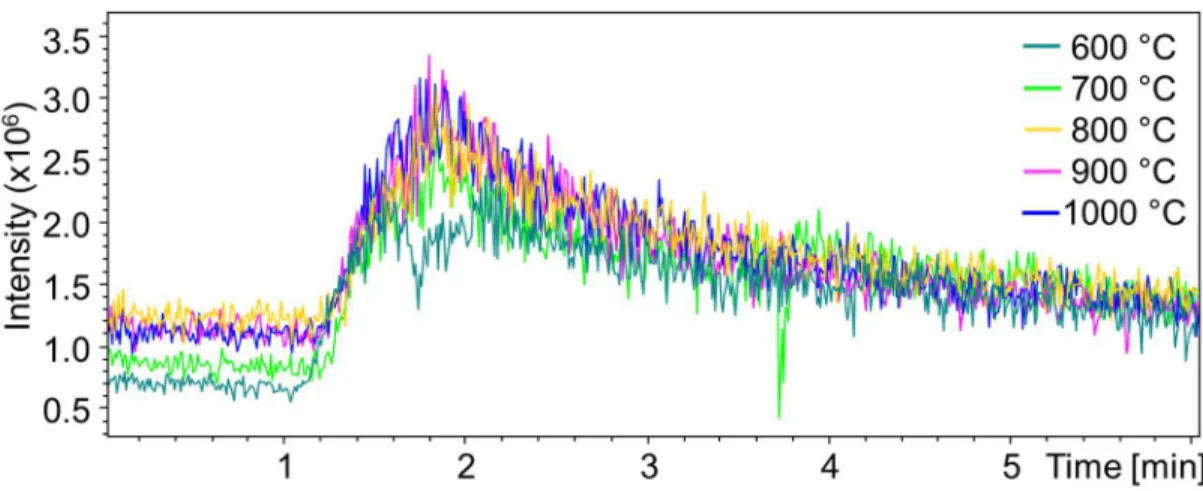
through the sample. Nonetheless, when a slow ramp rate (10 °C/s) is used to observe the pyrolysis of a sample of cellulose, the sample inside the tube changes color from white to brown at approximately 550 °C, indicated the onset of pyrolysis. Previous literature suggests 650 °C as the average temperature inside the pyrolysis region of a burning
cigarette, so 650 °C was the setting used for most experiments. Multiple temperatures were used to examine the effect of temperature setting on the pyrolysis of cellulose as shown in Figure 2.8. The total ion chronogram (TIC) over pyrolysis runs at temperatures of 600, 700, 800, 900, and 1000 °C suggest there is no difference in the total signal observed as a
function of temperature. Further, the mass spectrum obtained from each temperature setting is similar as displayed in Figure 2.9. The same peaks are observed in each spectrum and the absolute intensity of each peak does not change much as a function of temperature.
The setting for ramp rate in the heating program during pyrolysis was also studied by varying the ramp rate from 1 °C/s to 999 °C/s to a temperature of 650 °C. As shown in Figure 2.10 for 1 °C/s, pyrolysis occurs at 9 minutes and continues as the temperature reaches the maximum. For all others, pyrolysis occurs at approximately 0.5 minutes. This is evidence that the heating rate setting is the heating rate of the heater coil, not the sample. The heating rate of the sample is also a function of the gas flow rate through the system that acts to cool the sample as the heater coil warms the sample. The spectrum observed for each ramp rate was nearly identical. The area under the pyrolysis “peak” for the 1 °C/s ramp rate from 9 minutes to approximately 16 minutes is much larger than the area under any of the other peaks. This suggests that more aerosol is sampled from a single pyrolysis run at slow ramp rates. This is a way one could do an experiment that requires the
Figure 2.8. Time-resolved pyrolysis profiles of cellulose at varying temperatures.
2.3. Aerosol Particle Size Measurement
The scanning mobility particle sizing (SMPS) system used includes a differential mobility analyzer (Model 3080, TSI Inc., Shoreview, MN) and a condensation particle counter (Model 3022A, TSI Inc. Shoreview, MN)4,5. A polydisperse aerosol was directed to the inlet of the differential mobility analyzer (DMA) with a flow rate not exceeding 1 L/min. If the flow of the gas carrying the aerosol particles was greater than 1 L/min, a Swagelok tee with a gate valve was used to divert a portion of the flow. The particles are uniformly charged then separated in size by an electric field. The sized particles are then sent to the condensation particle counter (CPC) for detection. In the CPC, particles are sent through a condensation chamber where a saturated t-butyl alcohol vapor condenses onto the particles to increase the particle diameter for measurement by light scattering. The number density of particles is correlated in time to the DMA voltage to generate a plot of particle number density versus particle diameter. Particle statistics can then be determined using the Aerosol Instrument Manager (AIM) software by TSI Inc6. The version of the software used was AIM 9.0.0.0.
2.4. Mass Spectrometry
purposes of ESI or related techniques: Esquire 3000 Plus quadrupole ion trap mass
spectrometer (Bruker, Billerica, MA) equipped with an Apollo I ESI source (Agilent, Santa Clara, CA), HCT-Ultra quadrupole ion trap mass spectrometer (Bruker, Billerica, MA) equipped with an Apollo I ESI source (Agilent, Santa Clara, CA), LTQ-FT linear ion trap and fourier transform – ion cyclotron resonance (FT-ICR) mass spectrometer (Thermo Scientific, Waltham, MA) equipped with an Ion Max ESI source (Thermo Scientific, IQLAAEGABBFACTMAJI).
2.5. Ionization and Sampling 2.5.1 Electrospray Ionization
For the Esquire 3000 and HCT-Ultra mass spectrometers, the nebulizer used was either an Agilent (G1946-67098) or Bruker (A5940) nebulizer, both of which have nearly the same form factor for the Apollo I ESI source. For solvent delivery, a single-syringe infusion pump was used with various Hamilton gastight syringes. A schematic of an ESI nebulizer is shown in Figure 2.11. The solvent is delivered through a central capillary and the
was measured to be 90 °C using a Klein Tool MM400 and a bead wire type K temperature probe. For the Bruker instruments, the high voltage (HV) is applied to the inlet of the mass spectrometer while the nebulizer is held at ground. In positive mode, the inlet is held at a negative potential to attract ions of a positive charge. In most cases, this inlet capillary voltage was set to -5 kV for positive mode. In negative mode, the inlet is held at a positive potential to attract ions of a negative charge. In most cases, this inlet capillary voltage was set to +4 kV for negative mode. For ESI, the analyte was dissolved in a 1:1 mixture of methanol and water with acid (acetic or formic) added at 1% by volume unless otherwise noted.
2.5.2 Extractive Electrospray Ionization (EESI)
The ambient ionization and ambient sampling techniques used in the research discussed in this dissertation are all variants on ESI. Extractive electrospray ionization occurs when a plume of charged droplets interact with airborne droplets or aerosol particles7,8. For analysis of an aerosol, this is accomplished by intersecting a stream of analyte-containing aerosol particles with an electrospray plume to generate analyte ions9–11. A schematic of this interaction is shown in Figure 2.12. The source housing on the
Figure 2.12. Schematic of EESI setup.
exception of the data shown in Chapter 3, the arrangement shown in Figure 2.14 was used. The emitter is placed 7 mm away from the inlet to the mass spectrometer, orthogonal to the inlet capillary, with the tip of the nebulizer situated just above the inner ring of the spray shield. The aerosol outlet tube is placed on-axis with the inlet capillary at a distance of 10-15 mm. Just as in conventional ESI described above, the potential is applied to the inlet capillary. Because the source housing was removed, the electrospray nebulizer is no longer held at ground in this configuration, thus it must be manually grounded using a grounding strap attached from the body of the nebulizer to a grounded point on the mass
spectrometer. The electrospray solvent used in most cases was a 1:1 mixture of methanol and water with acid (acetic or formic) added at 1% by volume. This was altered in some studies to change the selectivity of the extraction by using different ratios, different solvents or different additives.
2.5.3 Coaxial Extractive Electrospray Ionization (Coaxial EESI)
To address the challenges associated with EESI, a new device was developed to simplify the setup and improve upon the operation of EESI in the standard configuration12. This device is used with the source housing intact and operation is similar to ESI. The absolute magnitude of the electrospray voltage in both positive and negative modes was increased by 1000 V due to the increased distance from the tip of the coaxial EESI nebulizer to the inlet capillary. Further details, including the construction and optimization of coaxial EESI parameters may be found in Chapter 4.
2.5.4 Open Port Sampling (OPSI)
results presented in this dissertation used ESI. Only initial testing for the use OPSI with APCI for the analysis of aerosols was done, but the use of OPSI-APCI for the analysis of other sample types is described elsewhere14–16. The OPSI-ESI device is used with the source housing intact. The construction and operation of the device is described in detail in
REFERENCES
1. TSI. Model 3076 Constant Output Atomizer Instruction Manual. (2005). 2. CDS Analytical. Pyroprobe 5000 Manual. (2012).
3. Spencer, S. E. Development of an Aerosol Mass Spectrometry System for the Analysis of the Composition of Aerosol Particles in Real Time. Ph. D. Dissertation (University of North Carolina, 2015).
4. TSI. Series 3080 Electrostatic Classifiers Manual. (2008).
5. TSI. Model 3022A Condensation Particle Counter Manual. (2002). 6. TSI. Aerosol Instrument Manager Software Manual. (2005).
7. Chen, H., Venter, A. & Cooks, R. G. Extractive electrospray ionization for direct analysis of undiluted urine, milk and other complex mixtures without sample preparation. Chem. Commun. 19, 2042–2044 (2006).
8. Law, W. S. et al. On the Mechanism of Extractive Electrospray Ionization. Anal. Chem. 82, 4494–4500 (2010).
9. Doezema, L. A. et al. Analysis of secondary organic aerosols in air using extractive electrospray ionization mass spectrometry (EESI-MS). RSC Adv. 2, 2930 (2012). 10. Gallimore, P. J. & Kalberer, M. Characterizing an extractive electrospray ionization
(EESI) source for the online mass spectrometry analysis of organic aerosols. Environ. Sci. Technol. 47, 7324–7331 (2013).
11. Swanson, K. D., Spencer, S. E. & Glish, G. L. Metal Cationization Extractive Electrospray Ionization Mass Spectrometry of Compounds Containing Multiple Oxygens. J. Am. Soc. Mass Spectrom. 28, 1030–1035 (2017).
12. Swanson, K. D., Worth, A. L. & Glish, G. L. A coaxial extractive electrospray ionization source. Anal. Methods 9, 4997–5002 (2017).
13. Swanson, K. D., Worth, A. L. & Glish, G. L. Use of an Open Port Sampling Interface Coupled to Electrospray Ionization for the On-Line Analysis of Organic Aerosol Particles. J. Am. Soc. Mass Spectrom. 29, (2018).
14. Van Berkel, G. J. & Kertesz, V. An open port sampling interface for liquid
introduction atmospheric pressure ionization mass spectrometry. Rapid Commun. Mass Spectrom. 29, 1749–1756 (2015).
CHAPTER 3: EXTRACTIVE ELECTROSPRAY IONIZATION
Portions of this chapter are adapted from the following reference with permission from Springer Nature.
Swanson, K.D., Spencer, S.E., Glish, G.L. Metal Cationization Extractive Electrospray Ionization Mass Spectrometry of Compounds Containing Multiple Oxygens. Journal of the American Society for Mass Spectrometry, 28(6). 2017. DOI: 10.1007/s13361-016-1546-2.
3.1. Introduction
Ambient ionization is a family of techniques that requires very few or no sample preparation steps and has become an important area of research in analytical applications using mass spectrometry1–5. Extractive electrospray ionization (EESI) is an ambient ionization technique in which a solvent is electrosprayed through a nebulized sample6–13. EESI is simple in design and can be implemented with most commercial electrospray ionization (ESI) sources8. It has also been shown that EESI can be used to sample from aerosols in real time as an alternative to aerosol collection, extraction, and derivatization followed by lengthy analysis by gas chromatography-mass spectrometry (GC-MS) or liquid chromatography-mass spectrometry (LC-MS)14,15. One area of interest in our lab is
characterization of aerosols formed in the pyrolysis of biomass16,17.
solvent composition in EESI18,23. In previous studies using EESI, the electrospray solvent typically contains a proton source (often formic or acetic acid)2.
3.2. Metal Cationization Extractive Electrospray Ionization Mass Spectrometry 3.2.1. Introduction to Metal Cationization EESI
Trace sodium is adventitious in electrosprayed samples and can increase the number of peaks in mass spectra and decrease sensitivity due to formation of [M+Na]+ in addition to the normal [M+H]+. The source of sodium in the sample is typically attributed to salts leached from glassware or impurities in analytical grade solvents24. To reduce cation formation, on-line desalting methods have been used25. However, the addition of metal salts to the electrospray solvent in ESI has been shown to enhance sensitivity in some cases, including the ionization of peptides26, ethoxylate surfactants27, polyether ionophores28, and carbohydrates29. In ESI, large carbohydrates are most efficiently ionized by large metals such as cesium; however, smaller carbohydrates such as sugars are more efficiently ionized by smaller metals, such as lithium30. One example of this effect is the analysis of
After ionizing by EESI, tandem mass spectrometry (MS/MS) of each metal cationized compound was investigated as a method to obtain more information on the structure of compounds than can be obtained from MS/MS of the protonated species. Metal cationization has been used to obtain structural information from collision induced
dissociation (CID) in the study of ginsenosides32, polyglycols33, monosaccharides34, disaccharides35, and polysaccharides36.
3.2.2. Unique Experimental Details
The electrospray solvent was a 1:1 mixture of water and methanol (v/v) prior to inclusion of an additive. For EESI with an acid, the additive used was acetic acid (Fisher, Hampton, NH) at a concentration of 175 mM. To study interactions with metals, sodium acetate, lithium acetate, potassium acetate, and silver trifluoroacetate were added to the electrospray solvent at concentrations ranging from 0.5 mM to 25 mM.
3.2.3. Metal Cationization EESI of Levoglucosan
Metal salts were individually added to the electrospray solvent for EESI-MS to ionize aerosolized levoglucosan and compare signal intensities. Protonated levoglucosan is observed in the mass spectrum when acetic acid is used as an additive with no trace of sodiated levoglucosan. When a metal salt was used as the additive for EESI, the
corresponding metal cationized levoglucosan was observed, with no protonated molecule, in the mass spectrum. The intensity of each metal cationized molecule observed was compared to the ion intensity of the protonated molecule measured when acetic acid was used as an additive (n=4). The same concentration of levoglucosan was used in the constant output atomizer for all experiments, thus any increase in signal intensity is related to an increase in sensitivity. When lithium was used as an additive, the signal for [levoglucosan+Li]+ (m/z 169) was 4.3 ± 0.9 times greater than the signal for [levoglucosan+H]+ (m/z 163) when acetic acid was used as an additive. Similarly, the signal for [levoglucosan+Na]+ (m/z 185) was 3.0 ± 0.7 times greater when sodium was used as an additive, and the summed signal for [levoglucosan+Ag]+ (m/z’s 269 and 271) was 1.5 ± 0.6 times greater when silver was used as an additive. Conversely, when potassium was used as an additive, the signal for
of [M+107Ag]+ and [M+109Ag]+. While the sensitivity of a single isotopic peak is slightly less than the protonated species, the isotope pair provides a characteristic signature in the mass spectrum. Compounds that have undergone silver cationization can easily be distinguished from other species by the isotopic peak doublet.
Lithium and sodium were found to increase sensitivity of levoglucosan detection much more than silver, thus experiments were carried out to separately determine the optimal concentration of lithium and sodium in the electrospray solvent to form metal cationized levoglucosan. The concentration of each metal additive was individually varied from 0.5 mM to 25 mM added to the electrospray solvents. In Figure 3.2, intensity of [M+X]+, where X represents the metal additive, is plotted as a function of metal


![Figure 3.2. Comparison of concentration profiles of both [M+Li] + and [M+Na] + for levoglucosan by EESI](https://thumb-us.123doks.com/thumbv2/123dok_us/8263201.2189118/67.918.225.692.400.682/figure-comparison-concentration-profiles-li-na-levoglucosan-eesi.webp)