Magellan/M2FS Spectroscopy of Galaxy Clusters: Stellar Population Model and Application to Abell 267

(1)

Magellan

/

M2FS Spectroscopy of Galaxy Clusters: Stellar Population

Model and Application to Abell 267

Evan Tucker1 , Matthew G. Walker1 , Mario Mateo2, Edward W. Olszewski3, John I. Bailey, III4, Jeffrey D. Crane5 , and Stephen A. Shectman5

1

McWilliams Center for Cosmology, Carnegie Mellon University, Pittsburgh, PA, USA 2

Department of Astronomy, University of Michigan, Ann Arbor, MI 48109-1042, USA 3

Steward Observatory, University of Arizona, Tucson, AZ 85721, USA 4

Leiden Observatory, Leiden University, P.O. Box 9513, 2300RA Leiden, The Netherlands 5

Carnegie Observatories, 813 Santa Barbara Street, Pasadena, CA 91101, USA

Received 2017 May 10; revised 2017 June 29; accepted 2017 July 30; published 2017 August 29

Abstract

We report the results of a pilot program to use the Magellan/M2FS spectrograph to survey the galactic populations and internal kinematics of galaxy clusters. For this initial study, we present spectroscopic measurements for 223 quiescent galaxies observed along the line of sight of the galaxy cluster Abell 267 (z~0.23). We develop a Bayesian method for modeling the integrated light from each galaxy as a simple stellar population, with free parameters that specify the redshift(vlos/c)and characteristic age, metallicity([Fe H]), alpha-abundance([a Fe]), and internal velocity dispersion (sint) for individual galaxies. Parameter estimates derived from our 1.5 hr

observation of A267 have median random errors of svlos=20 km s-1, sAge=1.2 Gyr, s[Fe H]=0.11 dex,

s[a Fe]=0.07 dex, andssint=20 km s-1. In a companion paper, we use these results to model the structure and internal kinematics of A267.

Key words:galaxies: clusters: individual(Abell 267)–galaxies: general– techniques: imaging spectroscopy

Supporting material:machine-readable table

1. Introduction

Galaxy clusters are the most massive gravitationally bound and collapsed structures in the universe, and therefore are important laboratories for observational cosmology(Diaferio & Geller1997; Dressler et al.2004; Voit2005; Jones et al.2009; Vikhlinin et al.2009; Rines et al.2013; Geller et al.2013). Due to their high density of galaxies they are also ideal for studying galaxy interactions and the effects these interactions have on the galaxy population. Galaxy clusters are studied in a multitude of ways, from gravitational lensing, both weak and strong (for example Kneib 2008; Applegate et al. 2014; Barreira et al. 2015; Gonzalez et al. 2015, and references therein), to X-ray temperature measurements of hot intracluster gas(Guennou et al.2014; Moffat & Rahvar2014; Girardi et al. 2016; Rabitz et al. 2017) to Sunyaev–Zeldovich effects (Sunyaev & Zeldovich1970; Churazov et al.2015), to optical spectroscopy(e.g., Rines et al.2003,2013; Hwang et al.2014; Stock et al. 2015; Biviano et al. 2016; Dressler et al. 2016; Tasca et al. 2016; Sohn et al. 2017, and references therein). Many of these methods seek to measure the mass and/or the mass function of the cluster, thus constraining cosmological parameters such as the amplitude of the power spectrum or the evolution of matter and dark energy densities over cosmolo-gical time.

With the advancement of multi-object spectrographs, astronomers now have the ability to conduct large spectro-scopic surveys of galaxies in cluster environments. Multiple-object spectroscopic systems have allowed for observations of hundreds of objects simultaneously. These spectrographs provide the necessary tools to perform efﬁcient follow-up of photometrically identiﬁed galaxies over a range of redshifts. For example, the Sloan Digital Sky Survey(SDSS)produced a spectroscopic catalog of millions of galaxy spectra with up to

1000 cluster member galaxies at low redshift and less than 10 member galaxies at their highest redshiftz~0.8(Ahn et al. 2012; SDSS Collaboration et al.2016). Additionally, the new age of spectroscopic data from SDSS includes integral field unit (IFU) observations with MApping Nearby Galaxies at Apache Point Observatory(MANGA), which resolves galaxy spectra in two dimensions on the sky. Using the 6.5m MMT and Hectospec fiber spectrograph, Rines et al. (2013) have measured redshifts for more than 22000 individual galaxies in 58 clusters (the HECs survey). Moreover, astronomers have used MMT/Hectospec and VLT/VIMOS to build large spectroscopic catalogs for cluster galaxies observed with the Cluster Lensing and Supernova Survey with Hubble(CLASH; e.g., Geller et al.2014; Biviano et al.2013; Rosati et al.2014; Girardi et al.2015). Another commonly used spectrograph, The Inamori-Magellan Areal Camera and Spectrograph (IMACS), is a multi-slit, wide-field spectrograph on the Baade-Magellan Telescope in Chile, and has been used in recent years to study galaxy clusters(Dressler et al.2011; Oemler et al.2013).

The Michigan/Magellan Fiber System (M2FS) is a multi-object ﬁber spectrograph consisting of 256 ﬁbers and was installed on the 6.5 m Clay Magellan Telescope at the Las Campanas Observatory in Chile in 2013 August(Mateo et al. 2012; Bailey et al. 2014). In its highest resolution setting (R~50000), M2FS was used by Bailey et al.(2016)to search for exoplanets in open clusters, used by Johnson et al.(2015a) to measure chemical abundances in globular clusters(see also Johnson et al.2015b,2017; Roederer et al.2016a), and used by Roederer et al. (2016b) to measure chemical abundances in dwarf spheroidal galaxies. At more moderate resolutions (R~18000) Walker et al. (2015a, 2016) and Simon et al. (2015) used M2FS for detailed kinematic analyses of dwarf spheroidal galaxies.

(2)

In addition to cosmological constraints from cluster masses, the galaxy spectra themselves convey a multitude of informa-tion about their stellar populainforma-tions. In recent years, with the development of more robust statistical techniques, there has been great progress in the fitting of galaxy spectra to extract stellar population information. These efforts have focused on building a more robust statistical framework around the early methods of stellar population synthesis (Tinsley 1972; Searle et al. 1973; Larson & Tinsley 1978) used for modeling the spectral energy distributions (SEDs) of galaxies. These early stellar population synthesis methods have been improved over the years to incorporate a more complete understanding of galactic processes(see Walcher et al.2011for a review). In the past few years, new efforts have been made to apply Bayesian techniques to fit these stellar population models. BayeSED (Han & Han 2014)and BEAGLE(Chevallard & Charlot2016) are two recently developed Bayesian models aimed at fitting SEDs of galaxies over a large wavelength coverage. However, these models are geared towards SEDs, which sample only a few band passes over a large wavelength range(fromγ-rays to IR). And most recently, Meneses-Goytia et al. (2015) developed a single stellar population model with Bayesian statistical techniques to fit spectra in the near-infrared.

In this paper we develop an integrated light population synthesis method forfitting galaxy spectra that is built upon the modeling techniques developed by Walker et al.(2015b). We applied this method to spectra, obtained in 2013 November, of Abell 267 (A267)with the Michigan/Magellan Fiber System (M2FS) on the Clay Magellan Telescope at Las Campanas Observatory in Chile. In Section2we describe the observations and subsequent data reduction. Section 3 describes the integrated light spectral(ILS)model used tofit these spectra. In Section4we describe how we implemented andfit this model and test it with mock spectra and previouslyfit galaxy spectra. In Section5we apply the model tofit the new A267 spectra.

2. Observations and Data Reduction

In this section we present a pilot program for cluster spectroscopy at low resolution with M2FS and detail the reduction of these spectra.

2.1. Target Selection

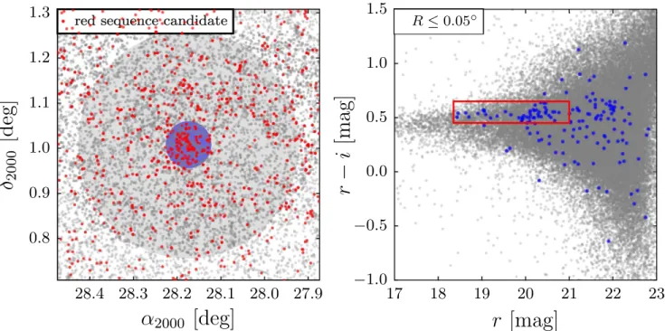
We select targets for M2FS observations by identifying galaxies detected in SDSS images(Data Release 12, Alam et al. 2015)that are projected along the line of sight to Abell 267 and are likely to be quiescent cluster members. First, we extract from SDSS all extended sources projected within a circle of diameter 0 . 5 that is centered on Abell 267(a2000=28 . 174 ,

d2000= + 1 . 008); for all such objects brighter than r=23,

Figure1 displays sky positions and r, r–i photometry. In the right panel of Figure1, the blue markers indicate colors and magnitudes for the galaxies closest to the center of Abell 267, i.e., those lying within the shaded blue circle (radius0 . 05 )in the left panel of Figure1. These objects clearly trace A267ʼs red sequence, which is enclosed by a red rectangle in the right panel of Figure1. Finally, the red points in the left panel of Figure1indicate the sky positions for all galaxies lying in the red sequence selection box. We consider all objects within this selection box to be candidate members of Abell 267ʼs red sequence. It is from this set of objects that we select M2FS targets, giving greater weight to brighter objects.

2.2. Observations

We observed 223 individual galaxy spectra on 2013 November 30 on the Clay Magellan Telescope using M2FS. We used the low-resolution grating on M2FS and chose a coverage range of 4600–6400Åwith a resolution ofR~2000. Of the 256 fibers available on M2FS, we allocated 223 for science targets, leaving 33 fibers directed at relatively blank regions of sky. We observed thefield over 6 subexposures of

(3)

15 minutes each, which we then stacked to improve the signal-to-noise ratio(S/N)and remove cosmic rays(see Section2.3 below). For wavelength calibration we took thorium–argon– neon lamp exposures both before and after a set of science exposures, and we took a quartz-lamp exposure immediately after the sequence of science exposures. To identify the apertures on the CCD for each fiber we took “fibermap” exposures, which are high S/N exposures of the ambient light in the dome during the daytime. For the purpose of calibration and correction for variations infiber throughput, we also took a series of high S/N exposures(including Th–Ar–Ne and quartz calibrations)during the evening twilight sky.

2.3. Data Reduction

The detector used with M2FS consists of two 4096×4112 pixel CCDs, each of which is read out through four amplifiers. We used the 2×2 binning setup for readout, so the output images are 2048×2056 pixels. The 256 fibers are organized into 16 cassettes of 16fibers each. The cassettes are spatially separated on the CCD and within each cassette each individual fiber is spatially separated. Figure2 shows an example of one of the CCDs with twilight spectra obtained during the A267 observations.

We use standardIRAFroutines to process the raw images, to extract the 1D spectra and to estimate the wavelength solution for each spectrum obtained in each science exposure. We also propagate the variance associated with the count level in each pixel of each image. At the outset, for every science frame(i.e., the images obtained in an individual science exposure) we generate a corresponding variance frame in which the value assigned to a given pixel is

= +

( ) C( )G R ( )

Var pix pix 2, 1

where C(pix) is the count in analog-to-digital units (ADU),

»

-G 0.68e ADU is the gain of the M2FS detector and

=

-R 2.7e is the read noise. In order to propagate variances, we process variance frames according to the way that we process their corresponding science frames (see below). For example, where we combine spectra via addition or subtraction (e.g., to combine subexposures or to subtract sky background) we compute the combined variances as the sum of the variances associated with the pixels contributing to the sum or difference. Or, where we rescale count levels in a given science exposure(e.g., to correct for the variability in theﬁber throughput)we rescale the variances by the square of the same factor.

For a given frame we begin the data reduction pipeline using theIRAFpackage CCDPROC to perform overscan corrections independently for each amplifier. We then rescale the counts in each frame by the gain associated with each amplifier independently in order to convert ADUs to electrons. For each of the two CCDs, we combine the four amplifier images to form a continuous gain-corrected image. We then bias subtract and remove the dark current. For the dark current correction, we rescale the measured dark current by the exposure time of each individual subexposure, then subtract this rescaled dark current. During our observations of A267, there was a non-negligible dark current that builds up in the corners of the CCD and contributed∼50–200 counts per 15 minute exposure.

Next, we use the IRAF package APALL to identify the locations and shapes of the spectral apertures, and to extract 1D spectra for science, quartz, Th–Ar–Ne arcs, and twilight exposures and associated variance frames. We initially identify aperture locations and trace patterns in the relatively bright

fibermap exposures. Fibermap exposures are obtained by taking short exposures, with all fibers plugged, of ambient sunlight in the dome during the daytime. We use fibermaps instead of quartz calibration frames to identify aperture locations because the ambient sunlight more uniformly illuminates all fibers, compared to quartz exposures. After identifying the aperture locations with the fibermaps, we use theIRAFpackage APSCATTER tofit the scattered light in the regions of the CCD outside the apertures and subtract thisfit from the regions of the CCD inside the apertures. Fixing the relative locations and shapes of the apertures according to the

ﬁbermaps, we use APALL and allow the entire aperture pattern to shift globally in order to provide the best match to the corresponding science frames. We apply exactly the same shift to deﬁne the apertures and traces for the Th–Ar–Ne frames. We then use APALL to extract the spectra from each aperture by combining (adding) counts from pixels along the axis perpendicular to the dispersion direction for each science, twilight, and Th–Ar–Ne and associated variance frames.

Next, we use the extracted twilight spectra to adjust for differences infiber throughput and pixel sensitivity. Wefirstfit a (6th-order) Legendre function to the extracted twilight spectra, which iteratively rejects counts that either exceed the

ﬁt by more than three times the rms of the residuals or are smaller than the ﬁt by more that 1.75 times the rms of the residuals. The lower tolerance is smaller than the upper tolerance to effectively exclude the absorption features from the

ﬁt. We then determine the median count level of theﬁt for each

ﬁber and normalize eachﬁt by the mean of these median count levels. Finally, we divide the science and twilight spectra by

(4)

this normalized fit per spectrum, thereby correcting for differences in throughput and pixel sensitivity simultaneously. Next, we estimate wavelength solutions, λ(pix). For each extracted Th–Ar–Ne spectrum, we use the IRAF package IDENTIFY to fit a (5th-order) Legendre polynomial to the centroids of between 30 and 40 identified emission lines of known wavelength. Residuals of thesefits typically have a root mean square(rms)scatter∼0.150Åor~10 km s-1_{. We assign}

the same aperture-dependent wavelength solutions to the corresponding science frames. Except for extraction from 2D to 1D, each individual spectrum retains the same sampling native to the detector; therefore, the wavelength solutions generally differ from one spectrum to another and have a non-uniformD Dl pix even within the same spectrum.

2.4. Sky Subtraction

After determining the wavelength solutions and correcting for ﬁber throughput and pixel sensitivity, we estimate the background sky and subtract it from our science exposures. Apart from a strong atmospheric emission feature at∼5600Å, the main source of sky background is scattered sunlight.

Following Koposov et al. (2011), we begin by taking the sky

ﬁbers (in this set of exposures ∼33) for a given frame and interpolate the individual sky spectra onto a common grid with constant spacingD ¢ Dl pix¢ ~0.1Å(oversampled by a factor of 16 with respect to the original sampling). For each discrete wavelength of the oversampled sky spectrum, we record the median count level and estimate the variance as

p

= ( )

N Var 2.198 MAD

2 , 2

sky

2

sky

where Nsky~33 and MAD is the median absolute deviation

(Rousseeuw & Croux1993). We then interpolate the resulting spectrum of median sky level and associated variances back onto the real, irregularly sampled wavelength solution that is unique to a given science spectrum. Lastly, we subtract the sky spectrum from the science spectrum, pixel by pixel.

Following sky subtraction, we then combine subexposures by taking the inverse-variance weighted mean at each pixel using theIRAFpackage SCOMBINE with the rejection routine CRREJECT (CosmicRayREJECT) to remove cosmic rays.

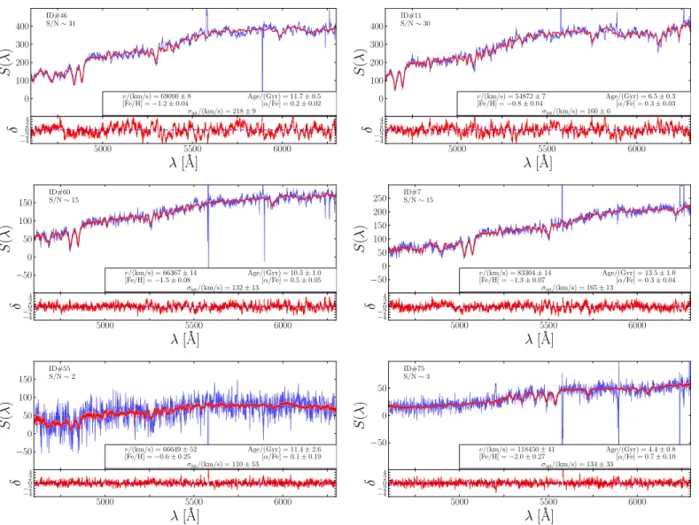
Figure 3.Sky-subtracted M2FS spectra(blue)for probable Abell 267 member galaxies(left panels)and contamination galaxies(right panel)spanning median signal-to-noise2S N pixel30. The red overplotted regions show the range of spectra encompassing the central 68% and 95% of the posterior PDFs(dark and light red, respectively)for our spectral model(Section3). The text in each panel lists the median S/N and our estimates ofvlos,Age,[Fe H],[a Fe], andsint, as well as the

ID#ʼs for easy reference to the data listed in Table3. The bottom portion of each panel shows the residuals of theseﬁts scaled by the variance in each pixel

(5)

Figure3 displays examples of the resulting M2FS spectra for science targets.

3. Integrated Light Population Synthesis Model for Galaxy Spectra

We model the galaxy spectra by generating synthetic integrated light spectra (ILS). This model is building on the procedure of Walker et al.(2015b; hereafterW15b), but here we are extending this model from resolved stellar spectra to integrated light spectra. The general procedure is to build a luminosity-weighted sum of template stellar spectra that correspond to a simple stellar population of a given age, metallicity, and alpha-abundance, and then to shift and smooth that spectrum to match the redshift, internal velocity dispersion, and instrumental broadening of the spectrograph.

3.1. Integrated Light Spectral Library

Theﬁrst component of the model is a stellar spectral library. We use the Phoenix Stellar Spectral Library (Husser et al. 2013)as the basis for building the integrated light spectra. This synthetic spectral library is computed on a regular four-dimensional grid in Teff, logg, [Fe/H], and [α/Fe] space

spanning a large range in each parameter: 0–15 Gyr in Age, 0 to 5 in logg, −4.0 to +0.5in[Fe H], and −0.2 to +0.8in

a

[ Fe]. We continuum-normalize each spectrum beforehand. This library does not include rare bright stars such as carbon or asymptotic giant branch(AGB)stars and therefore they will not be included in our model. Despite their rarity, the high luminosities of these stars can contribute signiﬁcantly to a galaxy’s integrated light(Conroy & Gunn2010). Because our model does not include the contribution of these stars, our parameter estimates are susceptible to systematic error that is not reﬂected in the quoted random errors.

In order to calculate an integrated light spectrum, we need to know how the stars from the stellar library contribute to the light in each stellar population; in other words we need to sum luminosity-weighted contributions along the isochrone for a given stellar population. For this we use the Dartmouth Isochrone Database (Dotter et al.2008).6This database consists of a three-dimensional grid of isochrone lists in galactic age, mean metallicity[Fe/H], and chemical abundance[α/Fe]space. We construct a regular grid of isochrone lists with DAge=0.25 Gyr, D[Fe H]=0.5 dex, and D[a Fe]=0.2 dex. Each isochrone is a list of stellar properties (mass, effective temperature, magnitudes, surface gravity) describing the stars of a given age, metallicity, and chemical enrichment.

We ﬁrst generate an integrated light spectrum for each isochrone, thus converting the isochrone database into an ILS library. For this procedure, we weight each individual library spectrum according to the luminosity function computed by Dotter et al. (2008). For each luminosity bin in the tabulated luminosity function, we identify the isochrone with a luminosity closest to the bin’s central value. For the luminosity function we use a magnitude bin width of 0.1 and a Chabrier log-normal initial mass function(IMF)of the form

s

µ ⎡

-⎣⎢

⎤ ⎦⎥

( )

( ) dN dM exp ln M M

2 , 3

c 2

2

where Mc=0.22M is the central mass ands=0.57 is the dispersion (Chabrier 2003). In principle these could be free parameters of our model as well, but for now we hold them

ﬁxed. We identify which stars listed in the isochrone fall within a given magnitude bin (from the luminosity function) and determine the stellar parameters (Teff, logg, [Fe H], and

a

[ Fe])associated with the median star within the bin. This star will be included in the integrated light spectrum with a weight that is simply the product of the number of stars in the magnitude bin calculated from the luminosity function and the luminosity of the star selected.

We denote the original spectra in the library as L0(l,

qatm), corresponding to stellar-atmospheric parameters qatmº

a

(Teff, log , Fe H ,g [ ] [ Fe]). As described by W15b (their

Equations(7)and(8)), we apply a smoothing kernel over the entire stellar library to obtain a unique spectrum at the speciﬁc qatm of each isochrone. We denote the smoothed spectra as

q l

( )

L1 , atm. In our case, the number of spectra in the Phoenix

library is NL=5566, and we set the smoothing bandwidths

equal to the grid spacing in each dimension: hTeff =200 K,

=

hlogg 0.5 dex,h[Fe H]=0.5 dex, andh[a Fe]=0.2 dex.

After generating each individual stellar spectrum q

l

( )

L1,i , atm,i corresponding to each isochrone, we weight and sum these spectra as described above, which produces an integrated light spectrum given by:

å

q q

l = f l

( ) ( ) ( )

L , L , w. 4

i N

i i i

ILS gal 1, atm,

The weight given to each spectrum iswiºnifi, whereniis the

number of stars in the given magnitude bin and f_i is the luminosity of the star speciﬁed in the isochrone;N_fis the number of magnitude bins in the luminosity function and qgalº(Age, Fe H ,[ ] [a Fe]) are the galactic parameters

speciﬁc to each isochrone. We do this for the entire isochrone database, thus generating an ILS library covering the parameter space deﬁned byqgal.

Whenﬁtting the galactic spectra there are two processes that broaden the absorption features: instrumental line spread function(LSF)and internal motions(i.e., redshift distribution, internal velocity dispersion, galaxy rotations, and so on). The instrumental LSF must be measured independently to break its inherent degeneracy with internal velocity dispersion (see Section 3.2 below). To mimic broadening, we add another dimension to our ILS library: a smoothing parameter h0.

Following the same procedure described byW15bto broaden the spectra over a range of smoothing bandwidths, we apply Equations (5) and (6) from W15b to each LILS(l,qgal). We

generate six versions of each integrated light spectrum using smoothing bandwidthsh0=0, 2, 4, 6, 8, 10Å. This range of

smoothing bandwidths was chosen to cover the broadening associated with the range of internal velocity dispersions we expect to measure in our galaxy sample(up to~550 km s-1_at

5500Å).

3.2. Spectral Model

Following Koleva et al. (2009), Koposov et al. (2011), and W15b, we ﬁt each individual galaxy spectrum with a

6

(6)

spectral model of the form

l = l l ⎛l +

⎝

⎜ ⎡_⎣⎢ ⎤_⎦⎥⎞_⎠⎟

( ) [ ( )] ( ) ( )

M S P T v

c

max l 1 los , 5

where cis the speed of light andmax[ ( )]S l is the maximum count level of a science spectrum. Equation(5)is the same as Equation (2) in W15b, except we chose to not include the polynomialQm( )l , which is a wavelength-dependent redshift.

We noticed from ﬁtting the A267 spectra that the parameters needed for this polynomial are unconstrained in our low-resolution integrated light spectra, but are relativelyconstrained by the high-resolution, resolved stellar spectra of W15b. We still included in this model the same form for the polynomial

l

( )

Pl given byW15b’s Equations(3), whichﬁts the continuum of the observed spectra.

Because we are modeling a population of stars, we build into our model a way of measuring the internal velocity dispersion of this population. The velocity dispersion will manifest itself as a broadening of the absorption features in each spectrum. However, this broadening will be degenerate with the LSF of the spectrograph, so care must be taken to break this degeneracy between the two sources of broadening. To do this, we ﬁrst measure the LSF with twilight spectra and then broaden the model spectra according to the LSF in addition to the broadening associated with the velocity dispersion of the stars. In order to allow for a wavelength-dependent LSF, we introduce another polynomial for the smoothing bandwidth,

l

( )

Hn , which we allow to vary with wavelength according to

l l l

l l l l l l l = + - + -+ -+ -⎡ ⎣⎢ ⎤ ⎦⎥ ⎡ ⎣⎢ ⎤ ⎦⎥ ⎡ ⎣⎢ ⎤ ⎦⎥ ( ) ( )

H h h h

h

... . 6

n

s s

n s

n

0 1 0 2 0

2

0

Given that the broadening related to velocity dispersionsint is

given bysint c= Dl l, wherecis the speed of light, the total

broadening associated with both the LSF and the internal velocity dispersion of the population of stars is given by

l =⎜⎛s l⎟ + l ⎝

⎞ ⎠

( ) ( ) ( )

h

c Hn . 7

2 int 2 2

This method introduces n +2 new free parameters: one for internal velocity dispersion and the other, n+1, from thehn

coefﬁcients. However, whenﬁtting twilight spectra, we assume thatsint=0 because the “stellar population”consists of only

the Sun,so we onlyﬁt then+1parameters associated with the LSF. On the other hand, whenﬁtting science spectra we use the previously measured n+1LSF parameters from the twilight

ﬁts,so weﬁt only forsint.

In order to let the spectral model vary continuously despite the library’s coarse gridding in galactic parameter space and the discrete values of the smoothing bandwidth, we apply another wavelength-dependent smoothing over the entire collection of library spectra. Speciﬁcally, for any choice of galactic parameters qgal and smoothing bandwidth h( )l , we obtain a

unique template

å

q l l l l = q q q q l l - -- -l

(

)

(

)

( ) ( ) ( ) ( ) ( ) T

L h K

K , , , , , , , 8 h h i N h h h i N h h h

ILS gal 0 3

3 i i i i h i i h ILS gal gal gal 0 gal gal gal 0

whereNILS=14202 is the number of ILS library spectra and

the kernel is

q q

l l

a a l

- -= - - + -+ - + -a ⎛ ⎝ ⎜ ⎞ ⎠ ⎟ ⎡ ⎣ ⎢ ⎢ ⎛ ⎝ ⎜⎜ ⎞ ⎠ ⎟⎟⎤ ⎦ ⎥ ⎥ ( ) ( ) ([ ] [ ]) ([ ] [ ]) ( ( )) ( ) [ ] [ ] h

K h h

h h h h h h h , , exp 1 2

Age Age Fe H Fe H

Fe Fe . 9 h i i i h 3 gal gal gal 0 2 Age2 2 Fe H 2 2 Fe 2 0 2 2 i i i

We set the galactic smoothing bandwidthshgalequal to the grid

spacing in each dimension:hAge =0.25 Gyr,h[Fe H]=0.5 dex,

= a

[ ]

h Fe 0.2 dex,hh=1Å. We found that setting the

smooth-ing bandwidthhh=2Å(the grid spacing of the library)results in

our model favoring a larger broadening parameter, thus over-smoothing the spectralﬁt; therefore, we decreased the smoothing bandwidth tohh=1Å, which solved this issue. This smoothing

procedure gives posterior probability distributions that are approximately Gaussian and tend not to cluster near the library’s grid points.

4. Analysis of Spectra

We now apply this model forﬁtting spectra and estimating model parameters.

4.1. Likelihood Function and Free Parameters

Given the spectral modelM( )l , we assume that the observed spectrumS( )l has a likelihood





q l p l l l l = - -= l ⎡ ⎣⎢ ⎤ ⎦⎥ ( ( )∣ ) [ ( )] ( ( ) ( )) [ ( )] ( ) S S S M S 1

2 Var exp 1

2 Var .

10 i N i i i i 1 2

In practice the value ofM( )li that we use in Equation(10)is the linear interpolation, at observed wavelength li, of the discrete model we calculate from Equation(5). This interpola-tion is necessary because a given template spectrum T( )l

retains the discrete wavelength sampling of the synthetic library, which generally differs from those of the observed spectra.

Following W15b in order to define the polynomials in Equations(5)and(6), we chosel=5 andn=2, respectively. These choices give sufficient flexibility to fit the continuum shape and to apply low-order corrections to the wavelength solution. We adopt scale parameters l0 and ls such that

 l l l 

-1 ( - 0) s 1 over the entire wavelength range

(7)

With these choices the spectral modelM( )l is fully speciﬁed by a vector of 14 free parameters:

q=( [ ] [a ] s

) ( )

v

h h h p p p p p p

, Age, Fe H , Fe , ,

, , , , , , , , . 11

los int

0 1 2 0 1 2 3 4 5

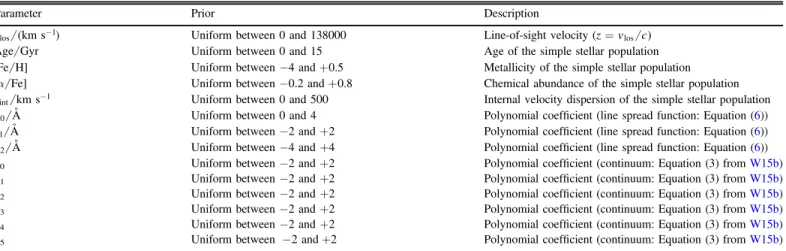
Thefirstfive have physical meanings and the rest are nuisance parameters. Table 1 lists all parameters and identifies the adopted priors, all of which are uniform over the specified range of values and zero outside that range.

4.2. Parameter Estimation

From Bayes’ theorem, given the observed spectrum S( )l, the model has a posterior probability distribution function (PDF)



q l l q q

l =

( ∣ ( )) ( ( )∣ ) ( )

( ( )) ( )

p S S p

p S , 12

where( ( )∣S l ,q)is the likelihood from Equation (10), p( )q

is the prior and



ò

q q q

l = l

( ( )) ( ( )∣ ) ( ) ( )

p S S p d ds ds1 2 13

is the marginal likelihood, or “evidence.”

In order to evaluate the posterior PDF, we must scan the 14D parameter space. For this task, we use the software package

MULTINEST7 (Feroz & Hobson 2008; Feroz et al. 2009).

MULTINEST implements a nested-sampling Monte Carlo algorithm that is designed to calculate the evidence (Equation (13)) and simultaneously to sample the posterior PDF(Equation(12)). Feroz & Hobson(2008)and Feroz et al. (2009)demonstrate thatMULTINESTperforms well even when the posterior is multimodal and has strong curving degen-eracies, circumstances that can present problems for standard Markov Chain Monte Carlo techniques.

4.3. Tests with Mock Spectra

As aﬁrst test of the accuracy of our model, we generated and

ﬁt mock spectra over a range of S/N values. Weﬁrst generated a noiseless mock spectrum, for a given set of Age,[Fe H],

a

[ Fe], andsint, using the pre-calculated spectral library (see

Section 3.1)and the spectral model described in Section 3.2. Table2shows the 20 sets of input galactic parameters we used to generate each noiseless mock spectrum. In order to also analyze the performance of our model at different S/N levels, we added noise such that the median S/N of each mock spectrum had values~1, 5, 10, 100. Therefore, each noiseless mock spectrum produced four noisy spectra, which we thenﬁt with our model. Each spectrum shown in Figure 4 was generated from the same noiseless mock spectrum (the input parameters for the mock spectra shown in Figure4are given in theﬁrst row in Table2).

Plotted over each mock spectrum in Figure 4 is the

best-ﬁtting model spectrum. We show in red the range of spectra attributed to the central 68% of the posterior distribution estimated by MULTINEST at each pixel. For high S/N levels, these red regions look just like single curves because theﬁts are tightly constrained; however, for low S/N, one can see the widths of these distributions(top left panel of Figure4). In the bottom portion of each panel, we show the residual difference

Table 1

Free Parameters and Priors for the Integrated Light Population Synthesis Model

Parameter Prior Description

-( )

vlos km s 1 Uniform between 0 and 138000 Line-of-sight velocity(z=vlos c)

Age Gyr Uniform between 0 and 15 Age of the simple stellar population

[Fe H] Uniform between−4 and+0.5 Metallicity of the simple stellar population

a

[ Fe] Uniform between−0.2 and+0.8 Chemical abundance of the simple stellar population

s _{km s}

-int 1 Uniform between 0 and 500 Internal velocity dispersion of the simple stellar population h0 Å Uniform between 0 and 4 Polynomial coefficient(line spread function: Equation(6)) h1 Å Uniform between−2 and+2 Polynomial coefficient(line spread function: Equation(6)) h2 Å Uniform between−4 and+4 Polynomial coefficient(line spread function: Equation(6))

p0 Uniform between−2 and+2 Polynomial coefficient(continuum: Equation(3)fromW15b) p1 Uniform between−2 and+2 Polynomial coefficient(continuum: Equation(3)fromW15b) p2 Uniform between−2 and+2 Polynomial coefficient(continuum: Equation(3)fromW15b) p3 Uniform between−2 and+2 Polynomial coefficient(continuum: Equation(3)fromW15b) p4 Uniform between−2 and+2 Polynomial coefficient(continuum: Equation(3)fromW15b) p5 Uniform between −2 and+2 Polynomial coefficient(continuum: Equation(3)fromW15b)

Table 2

Input Physical Parameters for the Mock Spectral Catalog

vlos Age [Fe H] [a Fe] sint

(km s−1₎ ₍_Gyr₎ ₍_dex₎ ₍_dex₎ ₍_{km s}−1₎

69579 10.9 0.39 −0.03 540

74406 5.8 −0.52 0.68 472

71331 9.0 −2.11 0.79 194

70380 10.8 −0.12 0.24 149

73100 13.2 −0.39 0.06 367

73851 14.9 −1.38 0.02 271

67592 0.2 −0.64 0.32 466

73442 2.8 −0.92 0.27 256

67467 3.1 −1.86 0.13 489

72545 7.9 −0.42 0.17 296

69134 8.7 0.60 −0.15 535

69698 1.4 −0.36 −0.10 204

68629 7.9 0.36 0.08 287

68724 14.4 0.36 0.20 519

71461 12.5 −2.38 0.63 507

68701 13.5 −0.38 0.58 534

73772 13.8 0.35 0.09 319

67092 1.4 −1.60 0.68 144

65444 3.2 −2.13 −0.04 365

67506 12.0 −2.13 0.51 364

7

(8)

between the best-ﬁtting spectrum (most likely set of para-meters) and the mock spectrum. The text within each panel indicates estimates of physical parameters redshift z, Age,

[Fe H],[a Fe], and internal velocity dispersionsint.

In the text of Figure4, along with the best-fit values of the galactic parameters, we also list their respective uncertainties. These uncertainties enclose the central 68% of the posterior PDF for each parameter. Therefore, in Figure 5 we show the marginal posterior PDFs for thefive galactic parameters, which better quantifies the distribution of each parameter. The posteriors shown in Figure 5 correspond to the spectral fits shown in Figure 4. Each color in the 1D and 2D posteriors corresponds to a different median-pixel S/N. The darker and lighter regions in the 2D posteriors show the 1s and 2s

contours of these distributions, respectively. For increasing S/N, the posterior distributions become more Gaussian in shape (which is expected considering that we use a Gaussian likelihood function Equation (10)) and the 2D posteriors are much better constrained. Furthermore, we also show the true input values of each of these parameters in purple. We can easily see how the posteriors converge on the true values as S/N increases. Additionally, we can see that some parameters are better constrained about the true values at lower S/N(vlos

for example), while other parameters([a Fe])have difﬁculty at low S/N.

We repeated this test for 20 sets of input parameters (Table2), and thus a total of 80 mock spectra. Figure6shows a summary of our results for the mock catalog. In each panel of Figure6, we show the difference between the true input value for each mock spectrum and the posterior PDFs for each of the

ﬁve galactic parameters. Each panel corresponds to a different parameter and the colors show how these distributions vary with S/N. As expected, with increasing S/N these posteriors become more constrained and are more centered on zero deviation(in other words centered on the true input value for the mock spectrum).

These tests establish good statistical properties for our model. However, they leave our estimates susceptible to systematic errors due to the choice of spectral library (e.g., incomplete line list)and isochrone databases(e.g., IMF).W15b found that there is a signiﬁcant dependence on choice of spectral library, such that estimates of[Fe H]and[a Fe]can suffer systematic errors of up to~0.5dex. In order to gauge the magnitude of these errors, we compare results obtained from our procedure with those obtained by others using different methods.

Figure 4.Mock spectra(blue)for different values of median S/N per pixel, which is identiﬁed in the top left of each panel. The original, noiseless mock spectrum is plotted in each panel in black. Overplotted in red in the top portion of each panel is the range of spectra encompassing 68% of the posterior distribution of the spectral

ﬁt. Also, in each panel we list the best-ﬁt parameters with uncertainties. Forvloswe show redshiftzinstead. In the bottom portion of each panel, we show the residual

(9)

4.4. External Tests

As a ﬁnal test of our model, we compared our model estimates with previously published results. The spectra for this test were generously provided by I. Chilingarian(2017, private communications) and we compared our results to those in Chilingarian et al. (2008) (hereafterC08). These spectra were observed on the ESO Very Large Telescope using the FLAMES/Giraffe instrument at a resolution of R~6300 in the wavelength range 5010–5831Å. Following the method outlined in Chilingarian et al. (2007), their spectral ﬁtting method is built upon the PEGASE.HR synthetic spectra (Le Borgne et al. 2004). Using a Salpeter IMF, they generated a

template spectrum from a linear combination of synthetic spectra at a given age and metallicity similar to our procedure. Using a multidimensionalc2_{minimization procedure, they}_ﬁ_rst

ﬁt the kinematics and continuum for each spectrum at a set of

ﬁxed values for age and metallicity. Finally, they obtained a map of minimalc2_{in age}_–_{metallicity space for each spectrum,}

from which they estimated age and metallicity for the given stellar population. Therefore, they estimated the stellar population parameters of age and mean metallicity along with line-of-sight velocity and internal velocity dispersion, all of which we compare to the output from our model. Furthermore, they measured Lick indices to compute magnesium abundance ratios[Mg Fe], which we compare to our estimates of chemical enrichment[a Fe].

Beforefitting the spectra, we noticed from manual inspection that one spectrum had strong emission lines, which we masked by setting the variance in those pixels to large values (109). Figure 7 compares the results between the two models: our results are on thex-axis(with the subscript“new”)whileC08 results are on the y-axis(with the subscript “old”). The solid black line overplotted in each panel guides the eye to a one-to-one relationship. For the velocity panel, we show the difference between measured velocities in order to more clearly show the distribution. We also fit a linear least-squares line to these distributions while fixing the slope to unity so that we can quantify any systematic differences between the two models.

Figure 5. Marginal posterior probability distributions for the five galactic parameters corresponding to thefits to mock spectra shown in Figure4. Each S/N value is represented with a different color, as indicated in the top right panel. For the 2D posteriors, we show the the 1σand 2σregions of these distributions as the darker and lighter regions, respectively. Above each column is the marginalized 1D posterior PDFs for each of thefive parameters. Also shown in each panel in purple is the input value of the parameters used to generate this noiseless mock spectrum.

Figure 6. Difference between all posterior PDFs and the true input values

(subscript true)for theﬁve physical parameters for all mock spectra. Each PDF is colored by the median-pixel S/N, as shown in the top left panel.

(10)

Theseﬁts are shown as the dashed black lines in each panel. In the bottom plot of each panel we show histograms of the differences between the two models, incorporating this systematic offset, and scaled by the total uncertainty in the measurements. In the bottom left panel we compare our measurements of chemical abundance[a Fe]to their measure-ment of [Mg/Fe]; therefore, this systematic offset partially correlates to the abundance of elements other than magnesium in the stellar population. The systematic offsets between our results and theirs is most likely due to differences in the choice of spectral libraries. We discussed above in Section 4.3 that different library spectra can affect the stellar property estimates by up to 0.5 dex. We caution the reader to understand that our estimates are susceptible to such systematic offsets.

The histograms show that our measured model parameters are mostly within ∼2 standard deviations of those measured inC08. There are a few outliers(one most notable in[Fe H]

space) that differ by 3s from the values cited in C08 after accounting for systematic offsets. These outliers arefits to low S/N spectra, and our model still produces goodfits to the data even though our best-fitting parameters differ from C08. Nevertheless, it is not surprising to see one or two3soutliers in a sample of ∼50. The distribution of the age comparisons appears to show little correlation; however, the histogram in that panel shows that our results are consistent withC08given the cited uncertainties. We would like to note that lacking the twilight spectra that would be necessary to estimate the instrumental LSF of C08, we do not compare sint for their

spectra.

5. Results for Abell 267

As a first application of our model, wefit new data of the cluster A267. In order to measure the LSF of M2FS, wefirstfit a set of twilight spectra. In doing so, we estimate the posterior probability distribution of each of the 3 hn parameters (see

Section 3.2). Because we observed one twilight spectrum for each of the 256ﬁbers of M2FS, we quantify the posterior PDFs

of the LSF for each fiber independently. Then, when fitting each of the science spectra, we sample the PDFs of the LSF that corresponds to the fiber where the science spectrum was observed. This technique quantifies the LSF and allows our

ﬁtting routine to break the degeneracy between the LSF and sint;furthermore, it also naturally propagates the uncertainty in

each of the hn parameters intosint for each galaxy spectrum.

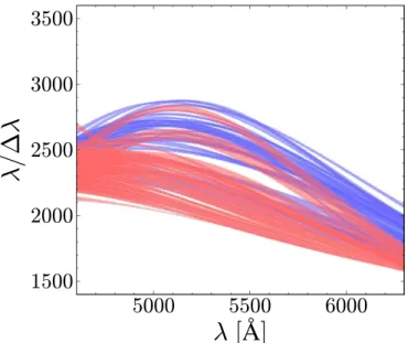
Figure 8 shows the resolving power R= Dl l for all the

ﬁbers used in this analysis. For eachﬁber we used the central 68% of the LSF covered by the PDFs determined by

MULTINESTto calculateR, which we plotted in Figure8. The two colors in Figure8correspond to the separate spectrographs that are used in M2FS. There is a clear dichotomy between the spectrographs, with the“blue”channel giving a systematically higher resolution; nonetheless,Ris roughly centered around the theoretical resolving power of M2FS at the low-resolution conﬁguration of∼2200.

Afterfitting all twilight spectra, we thenfit the sky-subtracted science spectra using the technique described in Section4above. Table3shows the results of thesefits for the galactic parameters. The parameter estimations are multidimensional posterior PDFs. Therefore, in Table3 we give the mean value of the marginal PDFs for each parameter, as well as the widths of these distributions(central 68%)shown as an error.

Figure 3 shows a series of sky-subtracted A267 spectra plotted in blue. Overplotted in red is the range of modelﬁts covering the central 68% of the posterior probability distribu-tion. Essentially, the red regions (thick red lines) show the width of the posterior PDF converted into a spectrum. The bottom panel of each plot shows the residuals scaled by the variance in each pixel. Here, we are only showing the residuals for the spectrum corresponding to the set of best-ﬁt parameters. The residuals scaled by the variance in each pixel are given by

d l l l

l

=

-( ) ( ) ( )

[ ( )] ( )

S M

S

Var , 14

whereS( )l is the sky-subtracted science spectrum,M( )l is the best-ﬁt model, andVar[ ( )]S l is the measured variance in the science spectrum. Also shown in each plot are the best-ﬁt galactic parameters along with their uncertainties, which are equal to the widths of their 1D posterior PDFs. To show the effectiveness of our model as a function of S/N, we arranged the plots with high median S/N per pixel in the top two panels (S N~30), to mid-level S/N in the middle (∼15), to low S/N in the bottom(∼2). Furthermore, the set of plots in the left column is for spectra with a high probability of membership to A267, while the spectra on the right are foreground and background galaxies.

In each of the plots in Figure3, we show the set of values for the galactic parameters corresponding to the best fit (highest likelihood) of the model to the data, along with their uncertainties. We display the multidimensional posterior PDF of thefive physical galactic parameters in Figure 9. Here, one can more easily see the effectiveness of our model to constrain the physical parameters of interest. For the 2D marginal PDFs, we once again show the1s and2s contours as the dark and light shaded regions, respectively, in each panel. Most of the PDFs in Figure9 are Gaussian in shape and therefore can be easily quantified by a mean(or a highest likelihood value)and a variance; however, some parameters (i.e., Age in Figure9)

(11)

have some Gaussian features. Because of this non-Gaussianity, it is better to describe the best-ﬁt parameters by a PDF instead of a single value and a variance. Having said that, we can still see in Figure 9 that the highest likelihood parameter values still estimate the mean of the posterior PDFs effectively and the variance in these values still gives a good approximation of the width of these distributions.

Figure 10 shows the error for each of the ﬁve galactic parameters labeled in the top right of each panel and median-pixel S/N as a function of r-band magnitude. We note the typical behavior for our observations: for fainter objects, median-pixel S/N decreases, while errors in measured quantities increase. The parameter estimates of A267 have median random errors of svlos=20 km s-1, sAge=1.2 Gyr,

s[Fe H]=0.11 dex,s[a Fe]=0.07 dex, andssint=20 km s-1.

All raw spectra, our spectralﬁts, and all posteriors attributed to these ﬁts are fully available online at the Zenodo database:https://doi.org/10.5281/zenodo.831784.

5.1. Comparison to Previous Redshift Results

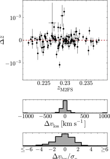
In order to discuss the accuracy of our A267 ﬁts, we compare our redshifts to those measured previously by Rines et al. (2013). In their paper they measured redshifts for over 22,000 galaxies from The Hectospec Cluster Survey (HeCS) and they cited 226 galaxy members to A267; we re-observe 114 of those galaxies. In Figure11we compare our measured redshifts (zM2FS) to theirs. In the top panel of Figure 11, for

added clarity we only show galaxies that are approximately at the redshift of A267 (z~0.23); on the other hand, the

Table 3

Results for Fitting of A267 Spectra

ID a2000 d2000 r i S/N vlos Age [Fe H] [a Fe] sint

(hh:mm:ss) (°:′:″) (mag) (mag) (km s−1₎ ₍_Gyr₎ ₍_dex₎ ₍_dex₎ ₍_{km s}−1₎

1 01:53:13.48 +01:00:48.6 20.38 19.86 10.1 114156±16 5.5±0.6 −0.72±0.10 0.05±0.05 193.3±12.2 2 01:53:20.26 +01:01:17.0 20.52 20.06 9.3 114059±18 6.5±0.4 −2.54±0.05 0.48±0.09 71.6±24.5 7 01:53:18.66 +01:05:8.6 20.12 19.64 15.5 83304±14 13.5±1.0 −1.32±0.07 0.34±0.04 165.1±13.0 11 01:53:28.58 +01:01:57.6 19.27 18.79 30.7 54872±7 6.5±0.3 −0.80±0.04 0.31±0.03 160.3±6.1 13 01:53:36.88 +01:03:50.8 20.13 19.63 5.0 66669±104 11.8±2.4 −1.29±0.25 0.34±0.18 298.6±84.3 19 01:52:59.68 +01:14:9.4 19.79 19.27 19.8 69207±11 11.4±0.8 −1.13±0.06 0.20±0.04 151.8±10.0 46 01:52:48.44 +00:58:44.8 19.43 18.91 31.2 69090±8 11.7±0.5 −1.19±0.04 0.16±0.02 218.2±9.4 55 01:52:31.17 +01:00:6.2 20.42 19.84 2.2 66649±52 11.4±2.6 −0.59±0.25 0.13±0.19 110.5±52.6 60 01:52:37.42 +00:59:2.2 19.62 19.06 15.8 66367±14 10.5±1.0 −1.53±0.08 0.47±0.05 132.0±12.5 75 01:52:20.13 +00:54:18.7 20.73 20.26 3.9 118450±41 4.4±0.8 −2.04±0.27 0.67±0.10 133.8±33.3

Note.

(This table is available in its entirety in machine-readable form.)

Figure 9.1D and 2D posterior probability distribution functions for theﬁve galactic parameters estimated for one of our A267 science targets(ID#46 in Table 3): line-of-sight velocity vlos, age, metallicity [Fe H], chemical abundance[a Fe], and internal velocity dispersionsintof the simple stellar

population. The dark and light shaded regions show the1sand2swidths of the 2D marginal posterior PDFs, respectively.

(12)

histograms in the bottom two panels show the distribution for all 196 repeat observed galaxies (separation< ´5 10-5 _deg₎_.

The top histogram panel shows the difference in the measured line-of-sight velocityDvlos, while the bottommost panel shows this difference scaled by the combined uncertainties in the measured redshifts sv. The histograms show that our redshift measurements are in good agreement with those measured by Rines et al.(2013).

6. Conclusions

We have introduced a new model for fitting galaxy spectra using a Bayesian approach and integrated light spectra. We chose to produce a new integrated light model for a few important reasons, which we highlight in the paper. The main reason is that we wish to implement this modeling in the Bayesian statistical framework offered by MultiNest, which allows us to fully quantify the covariances of all free parameters. Furthermore, our new model gives us theflexibility to alter any aspect of the model, from pre-calculated isochrones, to choices of synthetic spectral libraries, to the complexity of stellar populations, which would be difficult to implement with the previous population synthesis techniques.

In Section4.4, we showed that this model is able to adequately reproduce the results of previous stellar populationfits to A496 spectra, while increasing the flexibility for measuring the internal velocity dispersion of the stellar population. Lastly, this model robustly incorporates a wavelength dependencefit for the line-spread-function without the use of Hermite– Gaussian polynomials, which are typically used.

We outlined the process we used to generate an ILS library from a pre-calculated database of isochrones (Dartmouth Isochrones)and a library of synthetic stellar spectra (Phoenix Spectral Library). For this calculation, we assumed a Chabrier log-normal IMF withfixed scaling parameters, but the choice of IMF can be changed to incorporate different stellar evolution theories as well as allow the parameters or the model to be free. Furthermore, the choice of isochrones and stellar library can vary and one could use a library of real stellar spectra instead. We then discussed the model used tofit the galaxy operations and explained how wefit this model using the Bayesian nested-sampling algorithm MultiNest.

In order to test the statistical power of the model, we generated and ﬁt a mock catalog of galaxy spectra, thus quantifying the accuracy of the model. This showed that for increasing S/N, the model performs better; however, even for low S/N∼5, we are still able to reproduce the input galactic parameters with some level of precision. Furthermore, some of the galactic parameters are more easily estimated at lower S/N. For example, the velocity of the galaxy vlos can be estimated

from our model with a high degree of certainty over the full range of S/N tested with the mock catalogs; however, we achieved similar precision for the galactic age parameter at only high S/N values.

Following the analysis of the mock catalog, we applied the ILS model to new spectral data acquired from M2FS on the Clay Magellan Telescope. We ﬁt these spectra and estimated the posterior probability distribution for ﬁve galactic para-meters: vlos,Age,[Fe H][a Fe], andsint. We compared the

estimates of vlos to previously published measurements from

Rines et al. (2013), and found much agreement between the two measured redshifts.

In a companion paper, we will use our spectroscopic measurements to model the internal dynamics and galaxy populations of A267. In the companion paper we will apply a multi-population Dynamical Jeans Analysis. This model will simultaneouslyﬁt the dark matter and light distributions within the cluster while identifying contamination galaxies, substruc-ture within the cluster environment, and any overall cluster rotation.

We thank Margaret Geller and Ken Rines for helpful discussions that improved the quality of this work. We thank Charlie Conroy and Ben Johnson for useful discussions on incorporating wavelength dependence into the line-spread-function of the model. E.T. and M.G.W. are supported by National Science Foundation grants 1313045 and AST-1412999. M.M. is supported by NSF grant AST-1312997. E. W.O. is supported by NSF grant AST-1313006. We would also like to thank the anonymous referee for the helpful comments

ORCID iDs

Evan Tucker https://orcid.org/0000-0002-3542-8512 Matthew G. Walker https://orcid.org/0000-0003-2496-1925 Jeffrey D. Crane https://orcid.org/0000-0002-5226-787X

Figure 11.Comparison of the measured redshifts of each galaxy from our analysiszM2FSto previously published results in Rines et al.(2013). For clarity,

(13)

References

Ahn, C. P., Alexandroff, R., Allende Prieto, C., et al. 2012,ApJS,203, 21

Alam, S., Albareti, F. D., Allende Prieto, C., et al. 2015,ApJS,219, 12

Applegate, D. E., von der Linden, A., Kelly, P. L., et al. 2014,MNRAS,439, 48

Bailey, J. I., Mateo, M. L., & Crane, J. D. 2014,Proc. SPIE,9147, 91476P

Bailey, J. I., III, Mateo, M., White, R. J., et al. 2016,AJ,152, 9

Barreira, A., Li, B., Jennings, E., et al. 2015,MNRAS,454, 4085

Biviano, A., Rosati, P., Balestra, I., et al. 2013,A&A,558, A1

Biviano, A., van der Burg, R. F. J., Muzzin, A., et al. 2016,A&A,594, A51

Chabrier, G. 2003,PASP,115, 763

Chevallard, J., & Charlot, S. 2016,MNRAS,462, 1415

Chilingarian, I., Prugniel, P., Sil’Chenko, O., & Koleva, M. 2007, in IAU Symp. 241, Stellar Populations as Building Blocks of Galaxies, ed. A. Vazdekis & R. Peletier(Cambridge: Cambridge Univ. Press),175

Chilingarian, I. V., Cayatte, V., Durret, F., et al. 2008,A&A,486, 85

Churazov, E., Vikhlinin, A., & Sunyaev, R. 2015,MNRAS,450, 1984

Conroy, C., & Gunn, J. E. 2010,ApJ,712, 833

Diaferio, A., & Geller, M. J. 1997,ApJ,481, 633

Dotter, A., Chaboyer, B., Jevremović, D., et al. 2008,ApJS,178, 89

Dressler, A., Bigelow, B., Hare, T., et al. 2011,PASP,123, 288

Dressler, A., Kelson, D. D., Abramson, L. E., et al. 2016,ApJ,833, 251

Dressler, A., Oemler, A., Jr., Poggianti, B. M., et al. 2004,ApJ,617, 867

Feroz, F., & Hobson, M. P. 2008,MNRAS,384, 449

Feroz, F., Hobson, M. P., & Bridges, M. 2009,MNRAS,398, 1601

Geller, M. J., Diaferio, A., Rines, K. J., & Serra, A. L. 2013,ApJ,764, 58

Geller, M. J., Hwang, H. S., Diaferio, A., et al. 2014,ApJ,783, 52

Girardi, M., Boschin, W., Gastaldello, F., et al. 2016,MNRAS,456, 2829

Girardi, M., Mercurio, A., Balestra, I., et al. 2015,A&A,579, A4

Gonzalez, E. J., Foëx, G., Nilo Castellón, J. L., et al. 2015,MNRAS,452, 2225

Guennou, L., Biviano, A., Adami, C., et al. 2014,A&A,566, A149

Han, Y., & Han, Z. 2014,ApJS,215, 2

Husser, T.-O., Wende-von Berg, S., Dreizler, S., et al. 2013,A&A,553, A6

Hwang, H. S., Geller, M. J., Diaferio, A., Rines, K. J., & Zahid, H. J. 2014,

ApJ,797, 106

Johnson, C. I., Caldwell, N., Rich, R. M., et al. 2017,ApJ,836, 168

Johnson, C. I., McDonald, I., Pilachowski, C. A., et al. 2015a,AJ,149, 71

Johnson, C. I., Rich, R. M., Pilachowski, C. A., et al. 2015b,AJ,150, 63

Jones, C., Nulsen, P., Arnaud, K., et al. 2009, BAAS,41, 351

Kneib, J.-P. 2008, in A Pan-Chromatic View of Clusters of Galaxies and the Large-Scale Structure, Vol. 740, ed. M. Plionis, O. López-Cruz, & D. Hughes(Dordrecht: Springer),213

Koleva, M., Prugniel, P., Bouchard, A., & Wu, Y. 2009,A&A,501, 1269

Koposov, S. E., Gilmore, G., Walker, M. G., et al. 2011,ApJ,736, 146

Larson, R. B., & Tinsley, B. M. 1978,ApJ,219, 46

Le Borgne, D., Rocca-Volmerange, B., Prugniel, P., et al. 2004, A&A,

425, 881

Le Fevre, O., Vettolani, G., Maccagni, D., et al. 2003,Proc. SPIE,4834, 173

Mateo, M., Bailey, J. I., Crane, J., et al. 2012,Proc. SPIE,8446, 84464Y

Meneses-Goytia, S., Peletier, R. F., Trager, S. C., & Vazdekis, A. 2015,A&A,

582, A97

Moffat, J. W., & Rahvar, S. 2014,MNRAS,441, 3724

Oemler, A., Jr., Dressler, A., Gladders, M. G., et al. 2013,ApJ,770, 61

Rabitz, A., Zhang, Y.-Y., Schwope, A., et al. 2017,A&A,597, A24