DOI:10.1051/0004-6361/201525905 c
ESO 2015
Astrophysics
&
Mass distribution in an assembling super galaxy group at
z = 0.37
Merijn Smit
1, Tim Schrabback
2,1,3, Malin Velander
1, Konrad Kuijken
1, Anthony H. Gonzalez
4,
John Moustakas
5, and Kim-Vy H. Tran
61 Leiden Observatory, Leiden University, PO Box 9513, 2300 RA Leiden, The Netherlands e-mail:[email protected]
2 Argelander Institute for Astronomy, University of Bonn, Auf dem Hügel 71, 53121 Bonn, Germany
3 Kavli Institute for Particle Astrophysics and Cosmology, Stanford University, 382 via Pueblo Mall, Stanford, CA 94305-4060, USA 4 Department of Astronomy, University of Florida, Gainesville, FL 32611, USA
5 Department of Physics and Astronomy, Siena College, 515 Loudon Road, Loudonville, NY 12211, USA
6 George P. and Cynthia W. Mitchell Institute for Fundamental Physics and Astronomy, Department of Physics & Astronomy, Texas A&M University, College Station, TX 77843, USA
Received 16 February 2015/Accepted 26 July 2015
ABSTRACT
Aims.We present a weak gravitational lensing analysis of supergroup SG1120−1202, consisting of four distinct X-ray-luminous groups that will merge to form a cluster comparable in mass to Coma atz=0. These groups lie within a projected separation of 1 to 4 Mpc and withinΔv=550 km s−1and form a unique protocluster to study the matter distribution in a coalescing system.
Methods.Using high-resolution HST/ACS imaging, combined with an extensive spectroscopic and imaging data set, we studied the weak gravitational distortion of background galaxy images by the matter distribution in the supergroup. We compared the recon-structed projected density field with the distribution of galaxies and hot X-ray emitting gas in the system and derived halo parameters for the individual density peaks.
Results.We show that the projected mass distribution closely follows the locations of the X-ray peaks and associated brightest group galaxies. One of the groups that lies at slightly lower redshift (z≈0.35) than the other three groups (z≈0.37) is X-ray luminous, but is barely detected in the gravitational lensing signal. The other three groups show a significant detection (up to 5σin mass), with velocity dispersions between 355+55
−70and 530+ 45
−55km s−
1and masses between 0.8+0.4
−0.3×10
14and 1.6+0.5
−0.4×10 14h−1 M
, consistent
with independent measurements. These groups are associated with peaks in the galaxy and gas density in a relatively straightforward manner. Since the groups show no visible signs of interaction, this supports the hypothesis that we observe the groups before they merge into a cluster.
Key words.gravitational lensing: weak – galaxies: groups: general – galaxies: clusters: general – X-rays: galaxies: clusters – dark matter – galaxies: formation
1. Introduction
In the framework of hierarchical structure formation (Peebles 1970), matter overdensities grow through merging and accre-tion from the scales of galaxies up to those of large-scale struc-ture (LSS). In the concordanceΛcold dark matter (ΛCDM) cos-mology, the large-scale structure of the Universe is driven by the density fluctuations of dark matter, which provide the ini-tial framework for subsequent structure formation. As such, the mass distribution in the Universe is the driving force behind the formation of clustering sites for astrophysical processes, such as galaxy groups and clusters.
In galaxy formation and evolution, environment plays a role of major importance. Most galaxies are found in groups and clusters (e.g.,Eke et al. 2004), and observations indicate that the main part of galaxy evolution takes place in the group en-vironment, with significant post-processing occurring in clusters (Tran et al. 2008,2009, hereafter T08 and T09). A detailed un-derstanding of the total mass (dark and visible) and the structure of the mass density distribution is therefore necessary to under-stand both the processes of group and cluster formation and fun-damental scaling relations (e.g.,Leauthaud et al. 2010;Hoekstra et al. 2012;von der Linden et al. 2014) as well as to distinguish the latter from intrinsic variances in astrophysical processes.
Most overdensities are detected using visible, that is, bary-onic means. Common methods use galaxies (red sequence and spectroscopic association, e.g.,Eke et al. 2004;Gladders & Yee 2005) or gas (X-ray emission or the SZ effect, e.g., Sunyaev & Zeldovich 1970,1972;Finoguenov et al. 2007). While these methods are efficient, they might not always be as effective: they rely on the presence of baryonic matter, while the matter dis-tribution is driven by dark matter. Furthermore, the subsequent classification relies on observing the results of complex (astro-physical) processes, which introduces a significant intrinsic scat-ter in properties such as X-ray temperatures, star formation rate, and galaxy morphologies in different structures of comparable mass.
Gravitational lensing is the only direct probe of the total mass distribution, in the sense that it does not rely on astrophys-ical assumptions. A lower signal-to-noise ratio (S/N) makes it a less efficient detection method except for massive structures, but in combination with complementary methods, it is a pow-erful independent tool. From a statistical perspective, as an in-dependent, direct measurement, it can serve as a calibrator for mass-observable scaling relations (e.g., Leauthaud et al. 2010; Hoekstra et al. 2012;von der Linden et al. 2014). In individual systems it provides an independent estimation of the (projected) density field and can shed light on aspects such as interaction,
now identified in a robust manner, including examples of ac-cretion of smaller structures onto existing clusters. However, we have less observational evidence of the connection between structures on various scales, that is to say, the initial assembly of clusters from groups and galaxies. In this study, we perform a weak lensing analysis of SG1120−1202 (Gonzalez et al. 2005, hereafter G05), an assembling system of four galaxy groups at z∼0.37 discovered in the Las Campanas Distant Cluster Survey (LCDCS, Gonzalez et al. 2001). These groups are gravitation-ally bound and will merge into a galaxy cluster comparable in mass to Coma byz =0. The supergroup, hereafter SG1120, is confirmed by X-ray imaging and optical spectroscopy and has already formed a red sequence (see, e.g., G05, T08, T09, and Kautsch et al. 2008;Just et al. 2011;Freeland et al. 2011).
The individual subgroups are in the low-mass regime of X-ray groups,M200 ∼ 1013 to 1014 Mandσv ∼ 400 km s−1, and have not yet interacted. The aim of this study is to determine the total matter distribution in the system (dark and baryonic) and to constrain individual halo masses.
This paper is organized as follows. We summarize the gen-eral framework for weak lensing in Sect. 2. In Sect. 3 we briefly describe the data we use, while Sect. 4 covers the framework of measurement and analysis methods. In Sect. 5 we discuss the re-sults and the scientific implications. Section 6 gives a summary of our conclusions.
Throughout this paper we assume a Planck (Planck Collaboration XVI 2014) cosmology withΩM =0.3183,ΩΛ= 0.6817 andH0=67.04 km s−1Mpc−1.
2. Weak lensing framework
Gravitational lensing is the effect of curved space-time on the paths of light rays from distant sources to the observer as they pass through the potential of foreground structures. This geo-metrical effect leads to a displacement of point sources on the projected plane of the sky. The differential effect on extended sources leads to magnification and distortion effects. This is commonly described as a coordinate transformation
x y
=
1−κ−γ1 −γ2 −γ2 1−κ+γ1
x y
, (1)
where the trace componentκ is known as the convergence and the reduced symmetric part is determined by the gravitational shear (γ1, γ2).
Since we do not know the intrinsic source sizes or magni-tudes, we can only measure the net distortion or reduced shear (g1, g2)≡(γ1, γ2)/(1−κ):
x y
=(1−κ)
1−g1 −g2 −g2 1+g1
x y
, (2)
ple of background sources, these shapes will not be affected by gravitational lensing, but might be aligned with the potential of the structure under investigation. These effects are known as in-trinsic alignment (see, e.g.,Mandelbaum et al. 2006). However, recent results suggest that intrinsic alignments should have neg-ligible influence for current cluster weak lensing studies (Sifón et al. 2015).
The average measured distortion, corrected for systematic effects, can then be related to the projected density distribution in the lensing structure through
κ(θ)=4πG c2 Σ(θ)
DolDls Dos
, (3)
whereθrepresents the angular coordinates on the plane of the sky,Σ(θ) is the projected density distribution, andDiare the an-gular diameter distances between the observer, lens, and back-ground sources (luminosity distances, sometimes written asDl, are not used throughout this paper).
Normalized by 4πGc−2, the convergenceκis therefore also known as the dimensionless surface mass density, directly re-lated to the lensing density distribution and the lensing geome-try. For axisymmetric lenses,|γ|(θ)=κ¯(<θ)−κ(θ) with ¯κ(<θ) the mean surface mass density within a radial separationθ=|θ|to the lens centroid.
3. Data
For this project we made use of results of an extensive multi-wavelength data set (see, e.g., G05, T08, and T09).
Key to our lensing analysis are optical data, consisting of high-resolution HST/ACS1 imaging used for shape
mea-surements, as well as VLT/VIMOS (Le Fèvre et al. 2003), VLT/FORS2 (Appenzeller et al. 1998), and Magellan/LDSS3 spectroscopy.
We also used the X-ray temperatures based on Chandra/ACIS imaging and stellar masses inferred from VLT/VIMOS BVR photometry (T08) and complement our optical color information with KPNO/FLAMINGOS near-infrared (NIR)Ksimaging.
We useα=11h.19m.58s.0,δ=12◦0333.0 as center of coordi-nates, which roughly is the center of the VIMOS imaging data. To convert angular to physical separations, we use a reference redshift ofz = 0.37; this is the median of the redshifts of the four BGGs.
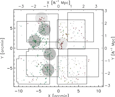
Fig. 1.Layout of the VLT/VIMOS pointings (red) and HST/ACS point-ings (blue). The detected X-ray peaks are shown as well (gray), with the radius of the circles 0.5h−1Mpc. The X-ray peaks 1 and 6 (light gray) are associated with structures at higher redshift, beyond SG1120 (G05).
3.1. HST imaging
The HST/ACS imaging data were taken in July 2005 and January 2006 and consist of ten pointings, forming a contiguous 11×18mosaic. Each tile was observed in F814W (0.05/pixel) for 2ks over four dithered exposures. Figure1shows the layout of the different pointings.
We reduced the data with the same pipeline as em-ployed inSchrabback et al.(2010), which usesMultiDrizzle
(Koekemoer et al. 2003) to stack exposures and remove cosmic rays. It also includes careful refinement of shifts and rotations between exposures as well as optimized weighting.
Schrabback et al. (2010) found that using MultiDrizzle
with the default cosmic-ray rejection parameters can cause cen-tral stellar pixels to be flagged as cosmic rays, especially when there are significant PSF variations between exposures. Galaxies are not affected, due to their shallower light profiles. To avoid differences in the effective stacked PSFs, we created separate stacks for stars and galaxies, with less aggressive cosmic-ray rejection for the former.
For a more detailed description of the reduction process, we refer toSchrabback et al.(2010).
3.2. Spectroscopy
We employed optical spectroscopy consisting of three subsets of data. The first subset of targets was selected from a magnitude-limited catalog (R ≤22.5), with preference given to objects in visually overdense regions (G05), and observed using VIMOS. Follow-up spectroscopy was selected from Ks catalogs (Ks ≤ 20) and carried out on LDSS3 and FORS2. Figure2shows the redshift distribution of the final target selection, using a redshift quality cut as defined in T08.
Members of the subgroups of SG1120 were initially selected as galaxies within 500 kpc of their respective X-ray peaks within the redshift range 0.32 ≤ z ≤ 0.39. We narrowed the redshift range to 0.34 ≤ z ≤ 0.38 without the loss of any members. Figure3shows a layout of the targets.
Fig. 2. Redshift distribution of the spectroscopic targets around SG1120. Three significant peaks are identified between 0.35 < z < 0.37, associated with SG1120; between 0.43<z<0.44, unassociated but concentrated slightly north of peak 1; and between 0.47<z<0.49, associated with X-ray peaks 1 and 6.
Fig. 3.Layout of spectroscopic targets, overlaid with the VLT/VIMOS pointings. (x, y) = (0,0) corresponds to α = 11.h19.m58.s0, δ = 12◦0333.0. Colors correspond to the peaks in Fig.2. The BGGs are indicated by larger circles.
3.3. Subgroups
In Table1, we give an overview of the properties of each sub-group, also given in G05, T08 and T09. We use the same num-bering convention for the X-ray peaks and BGGs as these papers. Subtle differences in the number of group members are due to using the same selection criteria as T09, but a slightly different cosmology.
Fig. 4.Radial (z, y) distribution of all objects (black dots, with a redshift quality of 3 as defined in T08). Objects within 500 kpc of an X-ray peak and the corresponding selection criteria are shown in different colors for easy distinction. The BGGs are indicated by larger circles, group redshifts by dashed lines.
4. Analysis
In this section we briefly describe our method of shape measure-ment. We discuss the redshift distribution and selection of back-ground sources. After establishing a reliable backback-ground catalog with robust shapes, we describe how we obtain a qualitative re-construction of the projected mass density and complement this with density profiles to the subgroups based on the BGG and X-ray peak positions.
4.1. KSB+ shape measurements
The art of measuring accurate galaxy shapes is an ongoing field of investigation, as witnessed, for instance, by the Shear TEsting Programmes and the GRavitational lEnsing Accuracy Testing (Heymans et al. 2006;Massey et al. 2007; Bridle et al. 2010; Kitching et al. 2012;Mandelbaum et al. 2015, hereafter STEP, STEP2, and GREAT08, GREAT10, and GREAT3). We make use of the KSB method (Kaiser et al. 1995), the most commonly used and tested technique in the past decade, and discuss its ap-plication to ACS data.
For this study we used the same approach as Schrabback et al.(2007,2010, the TS pipeline in STEP and STEP2) based on the implementation byErben et al.(2001). KSB uses the first-order effects of distortions induced by gravitational shear and
tion (PSF). The main source of variations of the ACS PSF is caused by changes in the telescope focus, causing spatial and temporal fluctuations (see, e.g.,Schrabback et al. 2007;Rhodes et al. 2007).
A common strategy is to map the distortions caused by the PSF using the shapes of foreground stars, but the average num-ber of stars in our ACS images is∼20–40. This leads to a poorly sampled PSF and an imperfect correction, causing significant residual distortions, especially detectable at the edges of the im-ages where the tiles overlap slightly. We therefore adopted the same strategy asSchrabback et al.(2010) based on a principal component analysis of the PSF variation in dense stellar fields.
Furthermore, deterioration of the ACS CCDs over time due to constant exposure to cosmic rays in space leads to an effect called charge-transfer inefficiency (CTI), causing charge trails in the CCD readout direction (e.g.,Rhodes et al. 2007;Massey et al. 2010;Schrabback et al. 2010). These effects will affect the measured shear pattern and the reconstruction of the projected density distribution, and it is therefore important to correct for them.
Here we applied the same parametric CTI model as de-scribed in Schrabback et al. (2010) for the correction of the KSB+polarizations.
After constructing the shape measurement catalogs, we ap-plied several common selection criteria and cuts. These crite-ria are based on simulations and quality flags of the detection and shape measurement pipelines, and they depend on the noise properties, on the variance and convergence of the model fits, and on the object and PSF size.
A list of the various selection criteria can be found in the Appendix. Sources that pass the criteria of all pipelines num-ber 7012, for a source density of ∼64 galaxies/arcmin2 with
MAG_AUTOmagnitudesi814<27.1.
4.2. Redshift distribution
We acquired spectroscopic redshifts for 497 objects in our cat-alogs. The spectroscopic targets were selected based on mag-nitude, and preference was given to visually overdense regions, which means that these spectroscopically confirmed members do not give a complete picture of the galaxy distribution in SG1120. The brightest confirmed supergroup member hasi814 = 17.5, while the spectroscopic survey remains >50% complete to i814=20.5 (T09). We find that confirmed supergroup members have numbers peaking between magnitudes 19.5<i814<20.0.
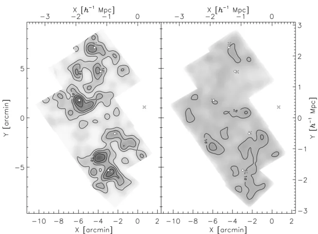
Fig. 5.Number density of sources withi814 <22 (left) andi814 >22 (right), smoothed using a Gaussian smoothing kernel with a width of 20. Dense regions are shown as dark in a normalized grayscale. Contours correspond to fluctuations in integer standard deviations in number density.
initially selected background sources as objects withi814 ≥ 22 and assessed possible contamination by faint foreground objects. Figure5shows the number density of sources withi814<22 and i814 > 22, where we have used a Gaussian smoothing with a 20kernel width.
Because gravitational lensing is a geometric effect that has a non-linear dependence on redshift, we took the expected redshift distributions into account, following the same parametrization as inSchrabback et al.(2010). We show the total redshift distribu-tion of sources withi814>22 in Fig.6. For a given lens redshift, such as in this particular system, the lensing signal has a lin-ear dependence on the lensing efficiencyβ= max{0,Dls/Dos}. We can therefore determine a mean lensing efficiencyβfor the sources with respect to each subgroup redshift.
As mentioned earlier, both X-ray peak 1 and 6 (G05) are as-sociated with structures at higher redshift (both 0.46<∼z<∼0.48). We must take the gravitational distortions caused by these back-ground structures into account when trying to isolate the signal from SG1120. We therefore also determined a mean lensing ef-ficiency for these structures.
We found average lensing efficiencies of β ≈ 0.52 for SG1120, corresponding to an effective background redshift ofzeff ≈0.88, andβ ≈0.42 for the two background structures, corresponding to an effective background redshift ofzeff ≈0.95.
4.2.1. Foreground contamination
An intrinsic redshift distribution of sources withi814 >22 im-plies that some of these objects are faint foreground sources or members of the SG1120 structure. Based on our parametric
redshift distribution, we estimate that∼9% of our background sources to lie in front of SG1120.
Foreground sources are not lensed by the groups. We account for this dilution effect by assigning β = 0 to this part of the redshift distribution in our definition of the lensing efficiency above.
This assumes a random field of view, which is not the case for our observations, with known overdensities atz ∼0.37 and z ∼ 0.48. However, Fig. 5 suggests no significant correlation between the distribution of these sources and the galaxy distri-bution of SG1120. To estimate possible variations in the number densitynof sources withi814>22, we derived an average num-ber density profile around the group centers, as shown in Fig.7. We used radial bins between 10 < θ < 95 to avoid the BGGs and the edges of the ACS coverage. We also considered only the group centers of groups 2 through 5, as group 6 is not entirely covered by the ACS pointings. Finally, we averaged the signal over all four subgroups to increase the S/N.
We then quantified the radial dependence of the galaxy num-ber density by fitting a parameterized profile given by n(θ) = (1+a/θ)nbg, withθin arcseconds and withnbg = 64/arcmin2 fixed. (In fact, if we allownbgto vary, we recovernbg = (64± 3)/arcmin2.) We founda=0.14±1.11, consistent with no trend in galaxy number density with radial separation from the lens centers.
Fig. 6.Parametric redshift distribution of sources withi814>22 (upper
panel) and the corresponding distribution in lensing efficiencyβ(lower panel). In theupper panel, the dashed green line corresponds tozeff ≈ 0.88 with respect to SG1120 and the dotted red line corresponds tozeff≈ 0.95 with respect to the two structures at higher redshift. In thelower panel, the dashed green curve shows the distribution inβwith respect to SG1120, withβ ≈0.52 (dashed green vertical line), and the dotted red curve the distribution inβfor the two structures atz =0.48, with β ≈0.42 (dotted red vertical line).
Fig. 7.Variations in galaxy number densitynas a function of radial distance from the lens positions, using the X-ray peaks (diamonds) and BGG positions (squares). Data points are slightly offset for clar-ity. Overplotted is the average number density of∼64 galaxies/arcmin2 of the whole ACS mosaic (black solid line) and the best-fit radial pro-file (dashed) with 1σerrors (dotted). The estimated effect of the lensing magnification,μα−1, is shown in grayscale, varying the slope of the lu-minosity function between 0< α < 3. Different shades in grayscale correspond to steps of 0.5×10¹⁴in group massM
200.
number density. Magnification increases both the observed flux of background sources, leading to an increase inn, and the solid angle behind the lenses, causing a dilution ofn(not to be con-fused with the dilution of the shear signal caused by unlensed foreground objects in the background source sample). It then depends on the slopeαof the luminosity function whether the lensing magnification causes a net increase or decrease in num-ber density byμα−1, whereμandαdepend of the source redshift. Both effects were shown byHildebrandt et al.(2009). A decrease could cancel the effect of unidentified group members.
We wish to obtain a rough estimate of the expected influence of magnification to check whether it is smaller than the statistical uncertainty. For this we ignored the redshift dependencies ofμ andαand considered a wide range 0< α < 3, which was sim-ply chosen to assess all possible variations in the magnification without making assumptions about the luminosity function. We used a group mass ofM200=1.0 × 10¹⁴, whereM200is defined as the total mass within a radius ofr200 of a halo, where the
number densities, BGGs, and X-ray peaks) is closely correlated with the underlying mass distribution. Second, we determine the density profile parameters for each subgroup, taking into account the effect of each subgroup and background structure simultaneously.
4.3.1. Reconstruction of the mass distribution
We used a Kaiser-Squires (KS, Kaiser & Squires 1993) in-version technique to reconstruct the surface mass density. We smoothed the data onto a rectangular grid, using a Gaussian smoothing kernel with a width of 20, equal to the smoothing used for the galaxy number densities in Fig.5.
We investigated possible systematic errors in our data by changing the phase of the shear by 12π, which corresponds to rotating the background galaxies by 14π. The distortion caused by weak lensing does not introduce a curl in the shear field, and the resulting reconstructed map should display only noise in the absence of systematic errors.
4.3.2. Density profile parameters
Earlier studies indicate that the groups are infalling for the first time and have not yet interacted, although X-ray measurements show a possible onset of interaction (G05). We considered the groups as individual overdensities with spherically symmetric density distributions and derived halo parameters for each group, including the background structure around X-ray peak 6.
We considered two types of density profiles and two possible choices of group centroids. We considered the Navarro-Frenk-White (NFW, Navarro et al. 1996) density profile and compared this to the singular isothermal sphere (SIS) model.
The SIS profile is determined by a single free parameter, the halo velocity dispersionσγ, where the subscriptγis used to dis-tinguish this parameter, derived from a two-dimensional model of the projected mass density, from other derivations of velocity dispersion, such as the one-dimensionalσzderived from the
red-shift distribution. The advantages of this profile are its simplicity and the linear dependence of the lensing signal on the squared velocity dispersion. The tangential component of the shear with respect to the group center is given by
γt(θ)= 2π
c2σ 2
γ
β
θ, (5)
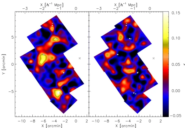
Fig. 8.Smoothed map of the reconstructed projected density distribution (left) and the imaginary control signal (right) where the shear signal is rotated out of phase. X-ray peak positions are indicated by white crosses and BGG positions by white circles.
The NFW profile is usually expressed in terms of its mass and concentration and depends on redshift. The halo massM200 is given by
M200≡200ρcrit(z) 4 3πr
3
200=100 H(z)
G r 3
200· (6)
The concentration c200 is defined as the relation between the characteristic shape of the density profile andr200. The analyti-cal formulas for the shear signal of an NFW profile can be found inWright & Brainerd(2000) andBartelmann(1996).
Because of the lower S/N, the centers of dark matter haloes should not be estimated directly from the lensing data when de-termining density profile parameters. Instead, one has to rely upon visible tracers such as peaks in the X-ray emission of hot gas or the brightest or heaviest galaxy (e.g., in terms of a stel-lar mass as derived in T08) in the group or cluster. If the fitted halo model is offset from the true underlying halo, the fit is in-ferior and the introduced systematic uncertainties can be signif-icant (George et al. 2012). In particular, the halo mass will on average be underestimated, while the uncertainties, most often determined from confidence levels, will be increased. This leads to both a biased and a less effective study.
As described in George et al. (2012), there are several choices possible as tracer of the halo center. These can be based upon a central galaxy, several or all of the associated galaxies, or the X-ray flux. In this study, the haloes under consideration are part of a coalescing system, and an offset from the true halo cen-ter of some or all of these tracers is not unlikely. However, the BGGs of the subgroup are also the most massive group galax-ies (MMGG,George et al. 2012) in terms of stellar mass and magnitudes in most observed bands and coincide well with the X-ray peaks (T08). We derived the parameter values using both options and determined whether these are consistent.
Given the close angular separation of the X-ray peaks, we did not compute azimuthally averaged profiles. Instead, we com-puted the total lensing distortiong =gifor each background
source induced by each of the six foreground structures. This is valid if we assume g 1, which is certainly the case for the sources where the distortion is not dominated by one of the lensing structures.
We then determined profile parameters for each subgroup using a χ2 minimization. For X-ray peak 1, we assumed σ = 820 km s−1from G05 and an order of magnitudeM
200 =3.7× 10¹⁴h−1Mand assessed the effect of omitting the influence of this background structure.
5. Results
In this section we discuss the reconstructed density distribution and best-fit profile parameters, and we show that SG1120 is con-sistent with expectations from hierarchical structure formation, even though the system is not relaxed.
5.1. Matter distribution
In Fig.8 we show the reconstruction of the projected surface mass density. We detect significant peaks near three of the fore-ground structures. We do not detect a significant peak in the density distribution near X-ray peak 2.
Fig. 9.Marginalized 2Dχ2distributions of the simultaneous fit to the in-dividual subgroup velocity dispersions, together with the marginalized 1D likelihoods for each subgroup. Overplotted are the 68.3%, 95.4%, and 99.7% confidence levels.
in a coalescing system. Finally, the map shows significantly stronger peaks than the control map.
5.2. Individual groups
5.2.1. SIS velocity dispersions
We present the results of the jointχ2minimization fit of SIS pro-file parameters around the X-ray peaks in Fig.9. The reducedχ2 value isχ2ν=1.4.
The combined contours of Fig.9show no features that in-dicate significant degeneracies between the individual group σγ values. While it is to be expected that nearby mass concen-trations influence the shear pattern around an individual lens, we conclude that noise is a dominant factor in these results. More massive haloes or smaller halo separations can be expected to increase correlations.
The resultingσγvalues are given in Table2. Consistent with
the reconstructed mass map in Fig.8, we do not detect a very significant lensing signal around X-ray peak 2, barely exceeding the 68% confidence limit.
The velocity dispersion associated with X-ray peak 1 is nec-essarily kept constant, as the peak lies outside the ACS mosaic. Upon inspection, it turns out that varying this parameter between 0≤σ1≤820 km s−1does not alter the results by more than 10% of the 68% confidence interval for X-ray peak 2, which lies clos-est to peak 1. The effect is even smaller for the other groups.
Similar to our assessment of systematics for the mass map reconstruction, we repeated the fit to a control signal by chang-ing the phase of the shear by12π. The results are consistent with a control signal ofgc≈0. Because of its less favorable lensing geometry (β = 0.42), the constraints for group 6 are weaker, although it is still detected at a significance ofσ≈1.6.
Finally, we determined how much our results would be affected if the signal were boosted by a dilution factor of
error bars are plotted at the vertical median.
1+(a+σa)/θ=1+1.25/θ for group member contamination,
as discussed in Sect. 4.2, using a conservative 1σ upper limit. We find that this does not alter the results by more than 37% of the 68% confidence intervals, justifying our earlier approach.
We repeated the fit around the BGGs as tracers of the halo centers. The results are very similar, with the fitted values also given in Table2. There is some difference with up to 2σ devia-tions between the results for peaks 3 and 5, where the separation between X-ray peak and BGG is also the largest. The quality of the fit, in terms of a reducedχ2value, is the same.
5.2.2.M200
In the same manner, we determined NFW profile parame-ters from the distortion pattern in the ACS field around the subgroups.
Weak lensing data of individual groups or low-mass clus-ters do not have sufficient S/N to provide useful constraints on M200 andc200 simultaneously. Therefore, we employed the mass–concentration relation given inMandelbaum et al.(2008), restricting the fit to one free parameter,M200. The results of these fits are summarized in Table2, both for the X-ray centroids and BGGs as tracers of the halo centers.
5.2.3. Scaling relations
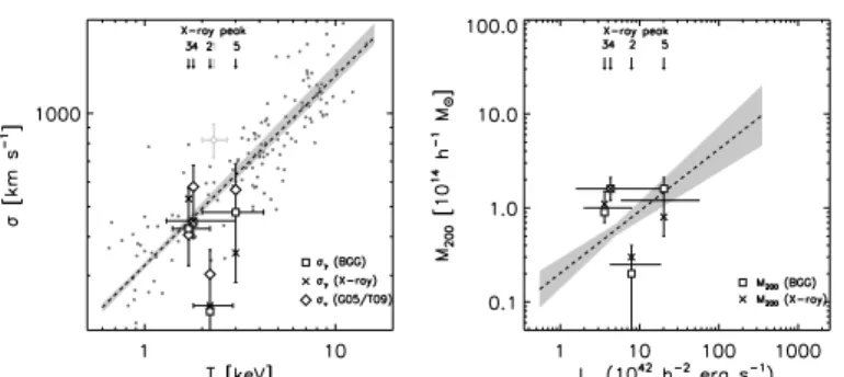
G05 showed that the subgroups were consistent with the lo-cal TX −σz relation (Xue & Wu 2000), a fact which did not
change with more spectroscopic data in T09. Here we did not determine 1D velocity dispersions from the redshift distribution of group members, but assumed the projections of 3D halo mod-els. Hence, we are not limited by group member identification. As mentioned before, group centroiding can be a problem.
Although the parameters of individual groups have shifted in this analysis, on average the groups still lie on the local TX−σzrelation, showing a scatter of similar magnitude as the
data inXue & Wu(2000, Fig.10).
Leauthaud et al.(2010) constrained theLX−M200 scaling relation using weak lensing data of groups in the COSMOS field. The supergroup as a whole is consistent with this scaling relation as well, within the scatter (Fig.10).
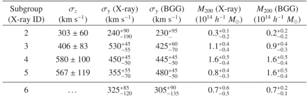
Table 2.Profile parameter fit results.
Subgroup σz σγ(X-ray) σγ(BGG) M200(X-ray) M200(BGG) (X-ray ID) (km s−1) (km s−1) (km s−1) (1014h−1 M
) (1014h−1M
) 2 303±60 240+90
−190 230+ 95
... 0.3+−00..12 0.2+ 0.2
−0.2 3 406±83 530+45
−55 425+ 60
−70 1.1+ 0.4
−0.4 0.9+ 0.4
−0.3 4 580±100 450+45
−50 445+ 45
−50 1.6+ 0.5
−0.4 1.6+ 0.5
−0.4 5 567±119 355+55
−70 480+ 45
−50 0.8+ 0.4
−0.3 1.6+ 0.5
−0.4
6 . . . 325+85
−120 305+ 90
−135 0.7+ 0.6
−0.5 0.7+ 0.2
−0.1
Even though individual groups do not always lie precisely on the determined scaling relations, differences in environment and their effect on the astrophysical processes behind the observ-ables used in these analyses create intrinsic scatter around these relations, which is averaged out in a stacking analysis such as employed inLeauthaud et al.(2010).
6. Summary
We have performed a weak lensing analysis of the coalescing supergroup SG1120 and showed that the underlying density dis-tribution of matter is well traced by both visual galaxy light and X-ray emission. The subgroups of SG1120 have not yet in-teracted, but are expected to do so within short timescales, as projected separations are of about 1–4 Mpc (G05). As such, the system is a unique demonstration of hierarchical structure formation.
Slight offsets between the peaks in the galaxy distributions, X-ray gas, and the total matter distributions are well within smoothing scales used and are consistent with an unrelaxed sys-tem on the verge of merging. We found that using either X-ray peaks or BGGs as tracers for the halo centers (George et al. 2012) has a minor impact on the derived halo parameters, with results consistent within 2σerror bars. We consider these con-clusions to be an indication of the robustness of our results.
Furthermore, while the groups are close enough to be gravi-tationally bound (G05), the individual group halo masses are low enough compared to their separations to treat them as individual lenses, within parameter error bars.
The fitted profile parameters are consistent with well-demonstrated scaling relations, within the intrinsic scatter cre-ated by astrophysical variations (Leauthaud et al. 2010). This is further confirmation that the observed structure of SG1120 is consistent with the paradigm of hierarchical structure formation, providing a unique example of this theoretical framework.
Structures such as SG1120 are rare. In fact, SG1120 should be seen as a single piece of a much larger puzzle, where con-firmation from studies of similar structures is a necessity. The structure of SG1120 is uniquely oriented in the plane of the sky, and the subgroups show no signs of interaction yet, mak-ing it well suited to distmak-inguish the various components and overdensities. An example of a well-studied heavier structure is the Cl 1604 supercluster (Gal et al. 2008), where the complex structure presents difficulties in determining accurate masses, ei-ther using spectroscopic velocity dispersions (e.g.,Lemaux et al. 2012) or weak lensing analyses of a few selected subclusters (Margoniner et al. 2005;Lagattuta 2011).
Especially the extension of studies like these to individual systems of lower mass like SG1120 will present a significant challenge, both in detecting such rare coalescing systems and
in obtaining robust and accurate lensing measurements, given the lower S/N. An interesting approach is the combination of large existing spectroscopic group catalogs (e.g.,Eke et al. 2004; Berlind et al. 2006;Tempel et al. 2012;Robotham et al. 2011) and recent or currently ongoing large sky imaging surveys of various width and depth, designed for lensing (e.g.,Heymans et al. 2012; Gilbank et al. 2011;de Jong et al. 2013) that are supported by extensive spectroscopic and color information. Acknowledgements. We thank the anonymous referee for constructive and ef-ficient comments that helped to improve this paper and the robustness of our conclusions. M.S. acknowledges support from the Netherlands Organization for Scientific Research (NWO). T.S. acknowledges support from the Netherlands Organization for Scientific Research (NWO), NSF through grant AST-0444059-001, and the Smithsonian Astrophysics Observatory through grant GO0-11147A. Observations taken by NASA HST G0-10499, JPL/Caltech SST GO-20683, andChandraGO2-3183X3.Facilities.VLT (VIMOS), VLT (FORS2), Magellan(LDSS3), HST (ACS), SST (MIPS), CXO (ACIS).
Appendix A: Quality flags and selection criteria for background sources
We assigned several quality flags to the source catalogs during detection and shape measurement.
We used the same rms noise model and deblending pa-rameters asSchrabback et al.(2010) for object detection with
SExtrator. In addition to detection flags, we required at least
eight adjacent pixels with values more than 1.4σabove the back-ground. We defined an initial S/N cut by flagging objects with
FLUX_AUTO/FLUXERR_AUTO<10.
We furthermore selected sources with a minimum size com-pared to the smearing induced by the PSF. We excluded sources for which the half-light radiusrh(as defined inErben et al. 2001) compared to that of the average star is not smaller than rh > 1.2rh∗.
Finally, we selected sources with a KSB shape measurement S/N (defined inErben et al. 2001) larger than 4, to be consis-tent with KSB+studies using a similar definition of the source S/N. In this pipeline, the effect of smearing and shearing by the PSF is for an important part described by thePgtensor. To avoid being dominated by noise, we excluded sources for which Tr(Pg)/2<0.1 (seeErben et al. 2001, for technical details and terminology).
In the final source selection, the catalog of 8273 galaxies is reduced to 7012,∼64 galaxies/arcmin2, that pass all quality criteria from detection and shape measurement.
References
Appenzeller, I., Fricke, K., Fürtig, W., et al. 1998,The Messenger, 94, 1
Bartelmann, M. 1996,A&A, 313, 697
Bartelmann, M., & Schneider, P. 2001,Phys. Rep., 340, 291
Heymans, C., Van Waerbeke, L., Bacon, D., et al. 2006,MNRAS, 368, 1323
Heymans, C., Van Waerbeke, L., Miller, L., et al. 2012,MNRAS, 427, 146
Hildebrandt, H., van Waerbeke, L., & Erben, T. 2009,A&A, 507, 683
Hoekstra, H., Mahdavi, A., Babul, A., & Bildfell, C. 2012, MNRAS, 427, 1298
Just, D. W., Zaritsky, D., Tran, K.-V. H., et al. 2011,ApJ, 740, 54
Kaiser, N., & Squires, G. 1993,ApJ, 404, 441
Kaiser, N., Squires, G., & Broadhurst, T. 1995,ApJ, 449, 460
Kautsch, S. J., Gonzalez, A. H., Soto, C. A., et al. 2008,ApJ, 688, L5
Kitching, T. D., Balan, S. T., Bridle, S., et al. 2012,MNRAS, 423, 3163
Koekemoer, A. M., Fruchter, A. S., Hook, R. N., & Hack, W. 2003, in HST Calibration Workshop: Hubble after the Installation of the ACS and the NICMOS Cooling System, eds. S. Arribas, A. Koekemoer, & B. Whitmore, 337
Schrabback, T., Erben, T., Simon, P., et al. 2007,A&A, 468, 823
Schrabback, T., Hartlap, J., Joachimi, B., et al. 2010,A&A, 516, A63
Sifón, C., Hoekstra, H., Cacciato, M., et al. 2015,A&A, 575, A48
Sunyaev, R. A., & Zeldovich, Y. B. 1970,Ap&SS, 7, 3
Sunyaev, R. A., & Zeldovich, Y. B. 1972,Comments on Astrophysics and Space Physics, 4, 173
Tempel, E., Tago, E., & Liivamägi, L. J. 2012,A&A, 540, A106
Tran, K.-V. H., Moustakas, J., Gonzalez, A. H., et al. 2008,ApJ, 683, L17
Tran, K.-V. H., Saintonge, A., Moustakas, J., et al. 2009,ApJ, 705, 809
van Waerbeke, L. 2000,MNRAS, 313, 524
von der Linden, A., Allen, M. T., Applegate, D. E., et al. 2014,MNRAS, 439, 2
Wright, C. O., & Brainerd, T. G. 2000,ApJ, 534, 34