The term structure and cost channel effect of monetary policy

(1)

The Term Structure and Cost Channel Effect of

Monetary Policy

by Myung-Soo Yie

A dissertation submitted to the faculty of the University of North Carolina at Chapel Hill in partial fulfillment of the requirements for the degree of Doctor of Philosophy in the Department of Economics.

Chapel Hill 2007

Approved by:

Dr. Richard Froyen, Advisor

Dr. Stanley W. Black, Committee Member

Dr. Michael K. Salemi, Committee Member

(2)

c

2007

(3)

ABSTRACT

MYUNG-SOO YIE: The Term Structure and Cost Channel

Effect of Monetary Policy.

(Under the direction of Dr. Richard Froyen.)

Sims (1992) first recognized a puzzling protracted rise in the price level following

a contractionary monetary policy shock. Two groups of studies have addressed this

“price puzzle”. The first group suggests that the price anomaly can be resolved by

adding future inflation information to the policy rule, because they believe that this

undesirable result comes from the omission of important information available to the

monetary authority. The second group regards this price response as normal because

of the cost channel effect of monetary policy.

Since the effectiveness of monetary policy depends critically on the correct

identi-fication of the policy transmission mechanism, the recognition of the existence of the

cost channel is important for the policy makers. This paper provides evidence of the

cost channel effect through a structural VAR analysis. Based on empirical evidence,

I construct a dynamic stochastic general equilibrium model, which addresses the cost

channel effect.

My model focuses on two related features by which monetary policy affects real

variables. (1) The model derives the term structure of interest rates, which states that

the monetary policy action changes the market’s expectations on the current and future

short rate path that, in turn, determine the long rates. Despite the closer relationship

of macro variables to long rates than to short rates, the monetary authority adopts

(4)

studies fail to take into account the direct impact of long rates on the economy. In

contrast, (2) my model highlights the role of long rates. I find that time lags in the

capital formation and long-term financing contracts by firms enhance the cost channel

effect, and generate the variables’ staggered responses. The monetary policy action

changes the short and long rates through the term structure of interest rates. Also the

firms’ borrowing pattern for both labor costs with short-term contracts and investment

projects with long-term contracts link the nominal short- and long-term interest rates

directly to firms’ marginal costs.

This paper incorporates a simple cash in advance feature, sticky prices and wages,

and habit formation. My model indicates that the price stickiness makes a limited

contribution to generate persistent responses, but the sticky wage amplifies the inertial

behavior of variables and ensures that the real wage responds in the direction that

the cost channel effect of monetary policy predicts. Contrary to the studies by Fuhrer

(2000) and Amato and Laubach (2004), in which they showed that habit formation

helps to explain the gradual response of macro variables such as output and inflation

to monetary policy shocks, habit formation in this paper only smoothes the response

(5)

To my wife, Hyunju Oh, for dedicating her time and effort to taking care of me and

(6)

ACKNOWLEDGMENTS

First and foremost, I am grateful and would like to thank professor Richard Froyen,

who is my advisor, for innumerable, thoughtful discussions on my thesis topics. Many

of important features in my model came from these discussions. Without Dr. Froyen,

this paper would not be what it is today. I would like to thank professor Michael K.

Salemi for allowing me the time to learn various techniques on policy analysis. I also

thank Hamilton Fout for many discussions and feedback. Finally, I thank my parents

(7)

LIST OF FIGURES

2.1 Autocorrelation functions of VAR residuals I . . . 26

2.2 Impulse response functions to the federal funds rate shock . . . 27

2.3 Impulse response functions to the federal funds rate shock with commodity price . . . 28

2.4 Impulse response functions of yields to the federal funds rate shock . . . 29

2.5 Impulse responses to a term premium shock . . . 30

2.6 Impulse responses to the federal funds rate shock: pre-Volcker period, 1965:Q2-1979:Q3. . . 31

2.7 Impulse responses to the federal funds rate shock: Volcker-Greenspan period, 1979:Q4-2005:Q4. . . 32

2.8 Impulse responses of yields to the federal funds rate shock: pre-Volcker period, 1965:Q2-1979:Q3. . . 33

2.9 Impulse responses of yields to the federal funds rate shock: Volcker-Greenspan period, 1979:Q4-2005:Q4. . . 34

3.1 Slope of yields over the business cycle . . . 50

3.2 Autocorrelation functions of VAR residuals II . . . 51

(11)

3.4 The first-step term premium responses for all maturity

yields to the contractionary monetary policy shock . . . 53

3.5 Term premium response to the federal funds rate shock for each maturity yield. . . 54

3.6 The first-step responses of the term premium for different maturity bonds to the negative output shock . . . 55

3.7 Term premium response to the negative output shock for each maturity yield. . . 56

3.8 The first-step responses of the term premium for different maturity bonds to the negative inflation shock . . . 57

3.9 Term premium response to the negative inflation shock for each maturity yield. . . 58

3.10 Effects of the macroeconomic shocks on the yield curve . . . 59

4.1 Impulse responses to monetary policy shock: Baseline model . . . 110

4.2 Two different inflation performances . . . 111

4.3 Limiting case of habit formation: ζ = 0 vs. ζ = 1 . . . 112

4.4 Without loan markets . . . 113

4.5 Without nominal rigidities . . . 114

4.6 Technology shock: ˆξt=ρξξˆt−1 +ξ,t . . . 115

(12)

(13)

LIST OF TABLES

2.1 Summary statistics of level data . . . 23

2.2 Summary statistics of filtered data . . . 24

2.3 Autocorrelation test result: H0 :ρ1 = 0 . . . 25

3.1 Autocorrelation test result . . . 48

(14)

Chapter 1 Introduction

Sims (1992) first recognized a puzzling protracted rise in the price level following a

contractionary monetary policy shock. Two groups of studies have addressed this

“price puzzle.” The first group, which includes works such as Sims (1992) and Leeper,

Sims, and Zha (1996), suggests that the price anomaly can be resolved by adding future

inflation information in the policy rule, because they believe that this undesirable result

comes from the omission of important information available to the monetary authority.

According to Hanson’s (2004) study, however, there is little correlation between an

ability to forecast inflation and an ability to resolve the puzzle. The second group,

such as Barth and Ramey (2001), regards this price response as normal because of

the cost channel effect of monetary policy. Following the second group, this paper

provides evidence of the cost channel effect of the monetary policy transmission through

a structural vector autoregression (VAR) analysis. Based on empirical evidence, I

construct a dynamic stochastic general equilibrium (DSGE) model which addresses the

prolonged co-movement of price responses with short rates.

Since the effectiveness of monetary policy depends critically on the correct

identi-fication of the policy transmission mechanism, the recognition of the existence of the

cost channel and the term structure channel is important for policymakers. As Ravenna

(15)

of nominal interest rates to the firms’ marginal costs.1 Christiano and Eichenbaum

(1992a) and Christiano, Eichenbaum, and Evans (2005, hereafter CEE) link a firm’s

financing cost of labor to the nominal short-rate. Li and Chang (2004) connect the

nominal interest rate to the production cost of capital by assuming that firms finance

business investment. Even though these studies successfully generate a cost channel

effect in the general equilibrium framework, they focus only on the short-term financing

cost.

Contrary to previous cost channel models, this paper emphasizes the role of long

rates for generating the cost channel effect and the persistent responses of the

econ-omy. This is based on the argument by Woodford (1999) and Kozicki and Tinsley

(2002) that macro variables are more closely related to long rates than short rates.

Therefore the term structure of interest rates is considered as an important monetary

policy transmission channel which connects the policy action to long rates. But

previ-ous macroeconomic models regarding a term structure relationship have mainly focused

on finding determinants of long rates and have paid less attention to the role of long

rates in the economy. The most well-known theory about the term structure of interest

rates is the expectations hypothesis, which states that the policy affects long rates by

changing the average of current and future short-rate expectations. But, as Ellingsen

and S¨oderstr¨om (2001, 2004) noticed, some puzzling results observed in the term

struc-ture data cannot be explained by the expectations theory. First, long-term interest

rates respond more strongly to monetary policy innovation than the expected path of

short rates does. Second, since an exogenous increase in short rates should lower

infla-tion in the long run, a positive relainfla-tionship between long and short rates is puzzling.

Third, even though the average relationship is positive, the relationship between long

and short rates varies over time. To resolve these puzzling results, recent studies such

(16)

as Ellingsen and S¨oderstr¨om (2001, 2004) and Beechey (2004) rely on the

asymmet-ric information between private agents and the monetary authority. This asymmetasymmet-ric

information creates an inference problem for private agents, and the private agents’

inference on unobserved shocks affects the expectation path of short rates, hence the

behavior of long-term interest rates.

On the other hand, Kozicki and Tinsley (2001) and G¨urkaynak et al. (2005)

em-phasize the shift in private agents’ views of long-run inflation to explain the observed

violations of the expectations hypothesis. They argued that long-term interest rates

are more closely related to the market’s expectations on long-run inflation, which is

one of the goals for the monetary authority to stabilize. From their view, the Fisherian

relationship between nominal interest rates and anticipated changes in prices is more

important in determining the long-term interest rates.

Even though the empirical evidence is mixed, Cook and Hahn (1989) show that, on

the average, the overall term structure of interest rates increases, but declines with

ma-turity when the monetary authority raises short rates, which supports the expectations

hypothesis of the term structure of interest rates. Their findings can be supported by

Edelberg and Marshall (1996), and Evans and Marshall (2002), who argued that the

long-rate responses following monetary policy shocks move in the direction that the

expectations hypothesis implies. Favero (2005) also showed that the combination of a

Taylor rule and the expectations theory provide considerable support for the

expecta-tions hypothesis of the term structure.

But these efforts to resolve the behavior of long rates are not fully based on the

micro foundation. Moreover, they are all silent about the long rate’s effect on the

economy. Evans and Marshall’s (1998) study successfully introduces the term structure

of interest rates into the general equilibrium framework. But, by assuming that there is

(17)

become redundant assets. Fuhrer and Moore (1995) analyze the role of wage contracts

with a term structure relationship. The aggregate demand equation in their model

links the output gap and the ex ante long-term interest rate which is calculated from

the term structure equation. Their analysis, however, is not fully based on the micro

founded model, and fails to explain how the long rate affects output and inflation.

The DSGE model developed here, on the other hand, focuses on two related channels

through which monetary policy affects the economy. First, the model utilizes the term

structure of interest rates as a monetary policy transmission channel. Monetary policy

actions in the model change the market’s expectations of the current and future short

rate paths, which consequently determine long rates. The model states that the

long-term interest rates are the sum of two parts: the average of expectations of current and

future short rates and the term premium. The term premium is assumed to follow an

exogenousi.i.d.stochastic process with no relation to a monetary policy shock or other

macroeconomic shocks. This assumption implies that short-term interest rate policy

affects long rates through the expectations hypothesis of the term structure. Some

empirical evidence about this assumption will be presented by examining the impulse

response functions of the term premium implied by the impulse responses of different

maturity yields to macro-economic shocks. Second, as a cost channel of monetary

policy, the change of both short and long rates affects macro variables such as output

and inflation. The direct impact of long rates on the economy is considered one of

the sources of staggered responses of macro-variables because the change of long rates

alters the firm’s long-run ability to produce output by investing in long-term investment

projects.

Time lags in the formation of capital stock and long-term financing contracts of

firms distinguish my model from previous cost channel models. They enhance the

(18)

time-to-build feature that my paper adopts is introduced by Kydland and Prescott (1982) to

explain aggregate investment behavior as an alternative model to a capital adjustment

cost model. A capital adjustment cost model is intensively studied by Lucas (1967),

Gould (1968), and Hayashi (1982), among others. While they fail both to separate

the long- and short-run supply elasticities of capital and to recognize time lags in

completion of investment projects, Kydland and Prescott (1982) argue that the

multi-period formation of capital stock is a crucial factor for explaining aggregate fluctuations.

Financial intermediaries in my model are assumed to facilitate economic activity by

providing interest-bearing assets to households and financing contracts to firms. Some

behavioral assumptions on the financial market participants are made in order to avoid

an identification problem while connecting the nominal short- and long-term interest

rates directly to firms’ marginal costs. These assumptions are based on the matching

principle, which states that the maturity structure of debt matches the maturity of

projects or assets held by profit-seeking economic agents. First, firms use both

short-term loan contracts, for financing the cost of labor used in the production process every

period, and long-term loan contracts for financing the whole cost of investment projects

that take multiple periods to be used in the production process. Second, financial

intermediaries allocate resources by matching maturities between the source of funds

and the use of funds. Third, the loan markets are perfectly competitive markets. As a

result, nominal returns on short- and term bonds are equal to the short- and

long-term borrowing costs to firms, respectively. Hence, long-long-term bonds are not redundant

assets.

There are many studies that try to explain why firms use different maturity

finan-cial contracts in their production process. These studies can be categorized into three

groups: an agent or contracting cost hypothesis, a signal or liquidity risk

(19)

debt maturity is used to control the conflict of interest between equity-holders

(stock-holders) and debt-holders (bond-(stock-holders). It predicts the inverse relationship between

the debt maturity and growth opportunities, i.e., investment. Firms with risky debt

(risky bond, hence vulnerability to default) have an incentive on behalf of

equity-holders to reject projects with positive but low present value. This happens because

even if equity-holders, the investment decision makers, undertake the entire cost of the

projects including the risk of bankruptcy, they receive only a fraction of the returns by

sharing it with debt-holders. In the view of equity-holders, debt-holders appropriate

parts of their benefit created from bearing default risk. Therefore equity-holders will

have an incentive not to undertake projects with positive present value whenever the

value is lower than the amount of debt issued. This under-investment incentive can

be reduced by issuing short-term debt, which matures before investment decisions are

made. Therefore, firms prefer short-term debt to long-term debt. Debt-holders also will

try to avoid such a suboptimal investment being realized by reducing the stated period

of loan (Barclay and Smith 1995, Stohs and Mauer 1996, and Morgado and Pindado

2003).

Second, a signal or liquidity risk hypothesis states that, with positive transaction

cost, lower-quality firms self-select into long-term debt if they cannot afford the cost of

rolling over term debt, and high-quality firms signal their type by issuing

short-term debt to minimize adverse selection cost (Barclay and Smith 1995, Stohs and Mauer

1996)). Firms with the highest and lowest credit risk issue short-term debt because

firms with the highest credit ratings have small refinancing risk, and firms with very

poor credit ratings are unable to borrow long-term because of the extreme

adverse-selection costs. On the other hand, firms with intermediate credit risk issue long-term

debt. Since lenders are reluctant to refinance the debt if bad news arrives, the firms

(20)

(Barclay and Smith 1995).

Third, the tax-based model predicts that the interaction of borrowers’ preferences

for accelerating interest tax shields and lenders’ preferences for delaying the recognition

of interest income can cause borrowers to prefer long-term debt when the yield curve is

upward sloping. Hence, companies will use more long-term debt when the yield curve

is upward sloping (Barclay and Smith 1995).

Without theoretical background, we can also find some evidence that firms use

long-and short-term debt in the production process in Demirg¨u¸c-Kunt and Maksimovic’s

(1999) study. They found by examining debt maturities of firms in 30 countries during

1980 and 1991 that large firms in developed countries have more long-term debt than

short-term debt. Moreover, small firms in countries with a large banking sector have

less short-term debt and their debt is of longer maturity. The authors conjecture

that the economies of scale of financial intermediaries in obtaining information and

in monitoring debtors would facilitate access to external finance, particularly among

smaller firms. They also find that the high ratio of net fixed assets to total assets is

positively correlated to the use of long-term debt, which implies that firms use their

fixed assets (as collateral) to obtain long-term debt.

The model incorporates a simple cash-in-advance (CIA) feature, sticky prices and

wages, and habit formation. In general, price and wage stickiness are thought to

gen-erate the persistent response of variables. But sticky wages turn out to be a more

important factor than sticky prices in deepening the inertial behavior and the cost

channel effect. Contrary to CEE (2005), who emphasize the role of variable capital

utilization to generate persistence in output and inflation, the time-to-build technology

and long-term loan contracts are crucial in my model. The studies by Fuhrer (2000)

and Amato and Laubach (2004) show that habit formation helps to explain the gradual

(21)

But habit formation in this paper only smoothes the response of consumption across

time.

The rest of the paper is organized as follows. In Chapters 2 and 3, the preliminary

data analysis of the US economy will be carried out using a structural VAR analysis.

The evidence of a cost channel effect for monetary policy transmission and the role

of the term premium in the term structure of interest rates shown in the US data

will be discussed in these chapters. Chapter 4 presents the dynamic stochastic general

equilibrium model, which addresses the prolonged co-movement of price responses with

nominal interest rates. This chapter also includes the policy simulation exercises based

on the model economy. The impulse responses of the model economy to monetary

(22)

Chapter 2 Preliminary Data Analysis of the

US Economy

In this chapter, the impulse responses of the US economy following a monetary policy

shock will be examined with a structural VAR method. The identification scheme and

the well known puzzle concerning price movements will be discussed. This chapter also

analyzes the direction of long-rate responses on different maturity bonds and examines

what generates these long-rate responses to monetary policy shocks.

2.1 Identification

Two points must be checked in analyzing the effect of monetary policy shock with a

VAR. The first is related to the stability of structural models. In general, the model

estimated under a specific regime cannot be used in different monetary policy regimes.

To avoid this problem, I re-do the impulse response analysis with two different

sub-sample periods: the Pre-Volcker period and the Volcker-Greenspan period.

The second point is related to the identification problem of the policy instrument.

The policy instrument consists of two parts: an endogenous or systematic relationship

(23)

exoge-nous policy shock. Correct identification of the systematic part is required because

the misspecification of the systematic part of the policy instrument produces puzzling

anomalies (Hanson 2004). Since the dynamic analysis of a VAR system may yield

reli-able information on the monetary transmission mechanism only after exogenous policy

actions are identified (Bagliano and Favero 1998), we also need to separate an

unfore-castable exogenous policy shock from the systematic part of the policy instrument.

Two different schemes for identifying the effect of policy innovation on the

non-policy variables can be considered. First, the central bank is assumed to observe only

past values of state variables when formulating the policy. That is, there is no feedback

from the economy to the central bank’s policy action within the period. We can achieve

this type of identification by ordering the policy variables first in the state vector. The

other identification method assumes that the central bank can observe current variables

as well as a history of the entire economy when it formulates the policy rule. Therefore

the central bank can react systematically to the change of current state variables.

This identification scheme can be achieved by placing policy variables after the current

observed state variables.

The model that I use for exploring the effect of the monetary policy shock adopts

the second identification scheme, which is employed by Christiano, Eichenbaum, and

Evans (1996, 1999). A VAR for ak×1 state vector of variables, Xt, is given by

Xt= Φ(L)Xt−1+ut, Eutu0t=V (2.1)

where L denotes a lag operator and ut is a vector of residual shocks whose

variance-covariance matrix is V. By pre-multiplying A0 on both sides of (2.1), the structural

(24)

where the structural shock vector et has a covariance matrix Eete0t = I. After

esti-mating (2.1) via ordinary least squares regressions, we can obtainA0 matrix using the

relationship between the covariance matrices ut and et, V = A−01A

−10

0 . That is, A0 is

the inverse of the lower triangular Cholesky factor of V.1

All variables that I use in this chapter are quarterly data from the FRED database

provided by the Federal Reserve Bank of St. Louise for macro-variables and from the

CRSP database for yields data. The state vector includes four types of variables: the

monetary policy instrument, contemporaneous inputs to the feedback rule, the yield

on a zero-coupon bond, and an additional explanatory variable. For the monetary

policy instrument, the federal funds rate (F Ft) is used. I assume that the feedback

rule incorporates contemporaneous values of the log of real gross domestic product

(RGDPt), the annualized inflation rate (P CEt) measured as the difference in logs of

the personal consumption expenditure deflator at time t and t−4, and the log of real

wages (RWt) measured by real compensation per hour in the business sector.

Long-rates (Y Tt) are used in a VAR one at a time with the 1- to 6-month, 1- to 5-year

and 10-year maturity yields.2 _{The quarterly financial data, the federal funds rate, and}

yields, are obtained by calculating 3-month averages of monthly data. Finally, the log of

non-borrowed reserves (N BRt) is used as an additional explanatory variable to measure

the demand for credit in the economy. This variable measures the implementation of

the federal funds rate target through open market operations (Edelberg and Marshall

1996). In summary, the state vector includes six individual variables and the ordering

is given by Xt = [RGDPt, P CEt, RWt, F Ft, N BRt, Y Tt]. All variables are de-trended 1_{This normalization on}_A

0satisfies the assumption that the monetary policy shock is orthogonal to

the information set of the monetary authority. Moreover, it ensures that the dynamic responses of the variables inXtare invariant to the ordering of variables in contemporaneous variables and additional explanatory variables (CEE 1999).

2_{A 10-year constant maturity yield is used for the 10-year yield from the Federal Reserve Bank of}

(25)

with the Hodrick-Prescott filter with a smoothing parameter of 1600 in order to see

the responses of deviations from the steady state values. The data go from 1965:Q2 to

2005:Q4 and 6 lags are included in each equation.3

The policy instrument F Ft, which is one element of Xt, can be decomposed into a

systematic component (the reaction function) and unforecastable policy shock. That

is,

F Ft=f(Ωt) +eg,t (2.3)

where eg,t denotes exogenous policy shock, and Ωt is a set of information available to

the monetary authority at time t that consists of two parts: contemporaneous values

of output, inflation, and real wage, and the entire history of the economy.

According to the theory of the term structure of the interest rates, market

expecta-tions about the future path of short rates induced by policy acexpecta-tions play a central role

in determining long rates. After observing the policy action, the market participants

form expectations about the future path of the short rates and formulate long-term

rates. For this reason, the long-term bond yields come after the policy instrument.

Since the feedback rule is a linear function of contemporaneous variables and lagged

values of all variables in the economy, the policy decision affects reserves and bond

yields contemporaneously and has an effect on the future realizations of all variables.

3_{I use data from 1965 because the policy instrument that I used here is the federal funds rate and}

(26)

2.2 Preliminary Analysis of the Data

In this section, I compute the first and the second moments of level data for two sample

periods to obtain preliminary information. The results are summarized in Table 2.1.

Panel A displays those with full sample data range, 1965:Q2-2005:Q4, and panel B

summarizes the moment properties within the Volcker-Greenspan period.

The average yield curve is upward sloping in both sample periods, and the standard

deviations of yields generally decrease as maturity increases. When we look up the

correlation coefficients between inflation and financial data including the federal funds

rate, we can see that the full sample period and the Volcker-Greenspan period are not

much different. The correlation coefficients between inflation and the federal funds rate

are similar across the two sample periods, with 61% in the full sample period and 69%

in the post-Volcker period. The amount of correlation between inflation and short-term

yields is similar, too, and decreases as maturity increases, even though the strength of

correlation between inflation and long yields in the full sample period is much smaller

than in the Volcker-Greenspan period. Specifically, the correlation between inflation

and longest-term yields (10-year) is -62% in the Volcker-Greenspan period, compared

to -45% in the full sample period.

The negative relationship between output and the financial data implies that when

the interest rates increase, output falls. It suggests that the interest rates can be

thought of as investment costs or production costs. The positive relationship between

inflation and the financial data confirms this interpretation that when interest rates

increase, the cost of production increases, hence the price goes up.

The correlations between output and financial data in the full sample period are

smaller than the correlations between inflation and financial data. But in the

Volcker-Greenspan period, the correlations between output and financial data are greater than

(27)

be-tween output and longest yield is -92% in the Volcker-Greenspan period and -19% in

the full sample period. From these results, we can conjecture that output and financial

data, including the federal funds rate, are highly positively correlated in the pre-Volcker

period, which is contradictory to the traditional belief that there is a negative

relation-ship between output and interest rate.

Table 2.2 shows the first and the second moment properties of de-trended data. Most

patterns resemble those from the level data. But the correlation coefficient between

output and financial data has a positive sign, which means that if the output gap

increases, then the deviations of yields from their trends also move in the same direction

as the output gap. The correlation of output or inflation with the yields decreases with

maturity in both sample periods. From this table, we can conjecture that the feedback

rule has positive signs for output and inflation gap because of the positive correlation of

the federal funds rate with output and inflation gap, 35% and 47%, respectively in the

full sample period; 46% and 27% in the post-Volcker period. The correlations between

financial data including the federal funds rate remain high relative to other variables.

Specifically, the correlations between the federal funds rate and 1-month yields are 92%

in both periods, but those correlations drop below 70% at 10-year yield in both periods.

2.3 Model Specification Test

In this section, I test the model specification by checking the autocorrelations in the

VAR residuals. Autocorrelation is frequently encountered in models estimated with

time-series data. Since error terms pick up the influences of variables affecting the

dependent variables that have not been included in the model, the persistent effect of

excluded variables causes the OLS estimation to be unbiased but inefficient. Moreover

(28)

section checks the model specification by testing serial correlation of VAR residuals

using the Lagrange multiplier test explained in Davidson and MacKinnon (1993).

We wish to test the null hypothesis that the errors ut in the model equation (2.1)

are serially independent against the alternative that they follow AR(p) process. The

test regression can be expressed as follows

ˆ

ut= ˜Φ(L)Xt−1+ p

X

j=1

ρjuˆt−j+u,t (2.4)

where ˆut is the vector of estimated errors from VAR. The matrix of regressors in the

original VAR equation is added because the lagged dependent variables in the regression

function (2.1) are included in Xt−1. It is known that when the original model includes

lagged dependent variables, the Lagrangian multiplier test should be applied based on

equation (2.4) (Verbeek 2000). A test statistic can be computed asT R2 whereR2is the

uncentered R2 from the OLS regression of ˆut upon their lags ˆut−1 and all explanatory

variables. T denotes the effective number of observations. It has aχ2 distribution with

pdegree of freedom under the null hypothesis. That is, if R2 is close to zero, it means

that the lagged residuals are not explaining current residuals.

Figure 2.1 depicts autocorrelation functions for each variable’s residuals from the

VAR estimation over 30 lags. Dotted lines represent±√T1.96. As shown in the figure,

the autocorrelation functions move within 95% confidence intervals, which implies no

serial correlation could be detected. Table 2.3 shows the serial correlation test results

for each residual when p = 1. The table also reports F-test statistics in comparison

with theχ2 _results. _F_{-test statistics for} _ρ

1 =ρ2...=ρp = 0 will have pand T −k−p

degrees of freedom where k is the order of VAR regression. Test results indicate that

when VAR(6) is applied, then there is no first-order serial correlation for all variables.

(29)

hypothesis of ρ1 =ρ2...=ρp = 0, in particular, for inflation. When I apply the χ2 test

usingT R2 for test statistics, the null hypothesis of inflation is frequently rejected after

p≥2. On the other hand, F-test states that inflation does not have serial correlation

when the residual equation has less than 5 lags. Overall, we can conclude that the VAR

specification with the 6th order does not bear the autocorrelation.

2.4 Impulse Response Functions

This section discusses the results of impulse responses to a monetary policy shock based

on the identification scheme explained in the previous section. The positive relationship

between interest rates and inflation will be discussed with the full sample period and

two sub-sample periods for concerning the stability of the empirical model.

2.4.1 Full Sample Period

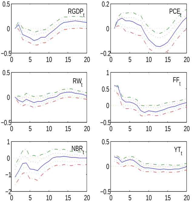
In Figure 2.2, the solid line denotes the impulse responses of state variables to

one-standard deviation exogenous monetary policy shocks for 20 quarters. The dash-dot

lines delineate 95% confidence intervals and the dotted lines depict 68% confidence

intervals. These were computed using a bootstrap Monte Carlo procedure outlined in

CEE (1999) with 1,000 bootstrap Monte Carlo draws. Five-year zero-coupon yields are

used to estimate impulse response functions to the contractionary federal funds rate

shock in Figure 2.2. The responses of variables with different yields are not different

from Figure 2.2.

The upper left panel depicts the output response to a contractionary federal funds

rate shock, and clearly shows the hump-shaped response. Output declines for

approx-imately six quarters with a maximum drop by 0.25%, then tends to rise. The federal

(30)

out before a year and a half. There is a persistent drop in non-borrowed reserves

(N BR). Together with the upward response of the federal funds rate, this result

im-plies that there is a significant liquidity effect in the economy. Real wages show an

insignificant but pro-cyclical response to the monetary policy shock. Its maximum

re-sponse is -0.11% six quarters after the shock, and it recovers the pre-shock level 13

quarters after the shock.

The upper right panel of Figure 1 represents the inflation response to a

contrac-tionary monetary policy shock. Inflation initially rises by 0.06% and tends to go down

six quarters after the shock. When we analyze the monetary policy impact in VARs,

many of these VAR specifications, particularly the ones without a commodity price,

frequently generate the price puzzle which states that the contractionary monetary

policy shock produces a substantial positive response of the aggregate price level for

many periods. The conventional wisdom predicts that the reduction of the volume of

non-borrowed reserves in the bank reduces the spending relying on bank credit. Hence,

aggregate demand and price also must fall.

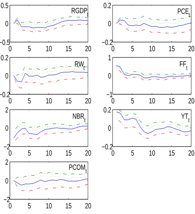
Figure 2.3 shows the impulse response functions to a contractionary monetary policy

shock when the state vector includes the commodity price index.4 _{According to Sims}

(1992) and Leeper, Sims, and Zha (1996), the exclusion of a commodity price can

result in a critical mis-specification of the model because it is important information

to policymakers when policy decisions are made. But, as indicated by the impulse

responses, even though the commodity price index is included in order to catch the

future inflation information of the monetary authority, its statistical performance is

only slightly improved, and the directional change is not observed. Hence, the claim by

Sims (1992), that the mis-specification of the policy rule5 _{induces the price anomaly, is}

4_{The spot market price index from BEA is used to measure the commodity price index.}

5_{Some studies, such as Hanson (2004), found that the policymaker’s information omitted in the}

(31)

hard to replicate.

Moreover, there are alternative explanations of the counter-cyclical movement of

prices such as that made by Chevalier and Scharfstein (1996). They focus on the test

of the null hypothesis that a firm’s markup is counter-cyclical when it is more financially

constrained with firm level data. They emphasize the role of capital market

imperfec-tions so that tighter liquidity constraints may generate counter-cyclical movement of

prices through markups. That is, the standard model predicts the lower marginal

prod-ucts in the boom implying lower marginal costs and factor prices. Hence the real factor

prices become lower in the boom. On the other hand, capital market imperfections and

a market share model can generate counter-cyclical movement of output prices relative

to factor prices. In periods of lower demand, firms tend to rely more heavily on external

financing as cash flow tends to fall faster than investment needs. Even if firms can raise

future profit by increasing market share as they reduce output price, external financing

firms are less inclined to reduce output price during economic downturns because the

increased probability of liquidation makes them care less about the future. Hence, they

have higher markups in recessions. Because of higher markups of externally financed

firms, an increase in the number of externally financed firms in recessions will make

markups even more counter-cyclical.

Another explanation of the price puzzle is the cost channel theory. When we

rec-ognize the cost channel effect of monetary policy, the co-movements of price and the

federal funds rate are not puzzling. As Barth and Ramey (2001) noticed, the

pro-cyclical response of real wages (RW) in Figure 2.2 is also the evidence of the

dom-inance of cost channel effect over the demand channel effect. A negative monetary

policy shock leads interest rates to increase. The increased interest rates, in turn, push

(32)

up the production cost by raising borrowing costs. The initial rise of price response to

the contractionary monetary policy shock reflects the dominance of the cost channel

effect relative to the demand channel effect. If a contractionary monetary policy has an

effect on the economy mainly through a demand channel, output and real wages move

in opposite directions because the decreased aggregate demand reduces output prices.

On the other hand, if a cost channel is dominant, both output and real wages should

fall because the decreased aggregate supply raises output prices. If both channels are

strong enough, the response of the relative price would not move unambiguously in one

direction.

The decrease of credit caused by the contractionary monetary policy shock reduces

the private sector’s demand for goods. The contractionary monetary policy shock also

raises the cost of current and future production because firms need to finance labor

and investments which will be used in the current and future production process with

higher interest costs. Hence, the upward movements of the price and the downward

movements of the output persist for some time. Therefore, the rise in inflation and the

fall in real wages may indicate that the cost channel of monetary policy transmission

dominates the demand channel in the economy.

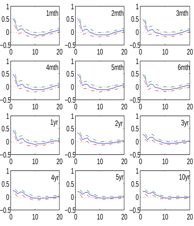
The direction of long-term yield response in Figure 2.2 is the same as the response

of the federal funds rates F Ft, but its effect is weaker than F Ft. Figure 2.4 shows the

impulse response functions (IRFs) of all bond yields to monetary policy shocks. Each

window represents a different yield (1- to 6-month, 1- to 5-year, and 10-year) starting

from the upper left corner and proceeding to the bottom right. Each impulse response

function is estimated by replacing Y Tt in the state vector with a different maturity

yield one at a time. The dashed lines delineate 95% confidence intervals. According

to the point estimates, the initial responses of all bond yields are significantly greater

(33)

These results are similar to those of Edelberg and Marshall’s (1996) study in that the

magnitude of the effect declines at longer maturities.

The initial responses of 4-year and longer-term rates persist for approximately six

quarters, which is slightly longer than the shorter-term bond yields. For example, the

impacts on 1-year bond yield and shorter yields disappear within three quarters at the

5% significance level. This can be interpreted in two ways. One is the asset market

imperfection from Andr´es, L´opez-Salido, and Nelson (ALN 2004). Since the asset

markets could have some frictions, investors tend to pay more money for purchasing

longer-term bonds. ALN considered the existence of transaction cost as an important

factor for the market friction. The other interpretation can be found in the studies

by Kozicki and Tinsley (2001) and G¨urkaynak et.al. (2005). They argued that the

change of long-term expectations on the inflation target by the central bank could

affect the movements of long-term interest rates via the Fisher equation. That is, the

movements of longer-term rates depend more on inflation expectations than on the

short rate expectations. Hence both studies assert that the effect on long rates could

remain over a longer horizon.

I will discuss the term structure of interest rates in a separate chapter by examining

the term premium responses implied by long-rate responses to macroeconomic shocks.

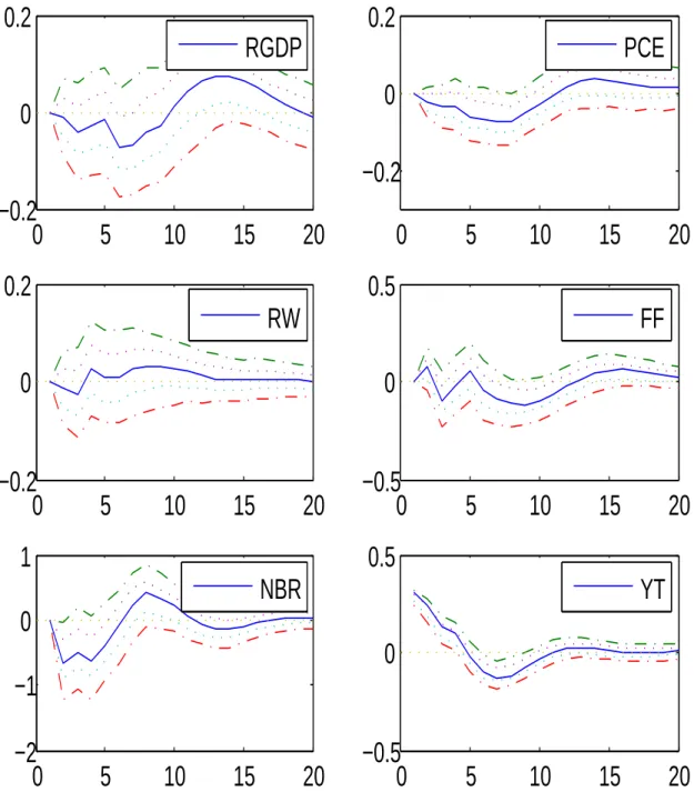
Here I examine the impulse responses to an asset market shock which can be thought

of as risk premium shock. Figure 2.5 shows the impulse responses of macro variables

to the longest-term (10-year) bond market shock. The risk premium shock does not

significantly affect output and inflation at the 5% significance level. The results are no

different when the long-term yield is ordered before the federal funds rate where the

central bank can be thought to have the asset market information when the policy is

formulated. This simply implies that the market participant fully absorbs the asset

(34)

assets.

The co-movements of interest rates and price indicate that the cost channel effect

dominates the credit channel effect, which suggests that the decrease of credit by the

contractionary monetary policy shock reduces the private sector’s demand for goods and

hence price level. The contractionary monetary policy shock causes the federal funds

rate and long-term interest rates to rise in the way that the expectations hypothesis

predicts. The increased short- and long-term interest rates raise the cost of future

production because firms need to finance investments which will be used in the future

production process. Hence the upward movements of the price level persists for some

time and the output decreases.

2.4.2 Sub-Sample Periods

Next, I examine the extent to which the impulse responses may change over the sample

period. To this end, I split the full sample into the period 1965:Q2 to 1979:Q3 (the

pre-Volcker period) and 1979:Q4 to 2005:Q4 (the Volcker-Greenspan period).

Figures 2.6 and 2.7 show the impulse responses of six variables to the contractionary

monetary policy shock in the pre-Volcker period and the Volcker-Greenspan period,

respectively. Again, the dashed line intervals and the dotted lines represent 95% and

68% confidence bands with the bootstrap Monte-Carlo procedure, respectively.

The results from the Volcker-Greenspan period are very similar to those from the

full sample period and initial inflation response remains positive four quarters after

the shock, which is shorter than the eight quarters in the full sample period. On the

other hand, the inflation response to the exogenous policy shock with the pre-Volcker

data fluctuates more across the entire forecast horizon than does that of the

Volcker-Greenspan period or the full sample period. Moreover, even if its initial response is

(35)

and cost channel effects are mixed; neither one appears dominant in the pre-Volcker

period. According to Hanson’s (2004) study, a price puzzle is related primarily to the

pre-Volcker sub-sample period and most indicator variables about the future inflation

information cannot resolve the price puzzle for this period. But my preliminary impulse

response analysis finds that, contrary to Hanson’s (2004) results, the demand and

cost channel effect are both strong enough in the pre-Volcker period, and the inflation

response during the Volcker-Greenspan period resembles the full sample response, which

implies that the cost channel effect is dominant in this period.

Figures 2.8 and 2.9 show the responses of yields to the contractionary monetary

policy shock in different sub-sample periods. Those results are very similar to the

full sample responses but the magnitude of the responses become smaller across all

maturities and the persistence of the effects is also shorter than that of the full sample

period. We can even see that the 5-year yields are significant only for the two-quarter

(36)

Table 2.1: Summary statistics of level data A. Full sample period, 1965:Q2-2005:Q4.

mean std corrl

πt f ft nbrt 1mth 1yr 5yr 10yr

yt 8.6932 0.3517 -.4484 -.3227 .9265 -.3276 -.3374 -.2420 -.1900

πt 4.0660 2.6647 .6114 -.4932 .6043 .5711 .4755 .4519

f ft 6.6082 3.3079 -.3246 .9779 .9671 .8864 .8525

nbrt 3.2885 0.5279 -.3276 -.3138 -.1906 -.1375

1mth 5.6412 2.6358 .9757 .8958 .8600

1yr 6.4810 2.7731 .9513 .9186

5yr 7.1266 2.4459 .9922

10yr 7.4735 2.4385

B. Volcker-Greenspan period, 1979:Q4-2005:Q4.

mean std corrl

yt 8.9114 0.2307 -.6182 -.8236 .7324 -.8062 -.8536 -.9105 -.9167

πt 3.2792 2.3396 .6883 -.6556 .6783 .6651 .6238 .6224

f ft 6.6837 3.8008 -.8068 .9847 .9798 .9258 .9091

nbrt 3.6252 0.3324 -.7888 -.7963 -.8140 -.8204

1mth 5.6735 3.0824 .9782 .9242 .9027

1yr 6.5662 3.2912 .9692 .9502

5yr 7.4499 2.8784 .9948

10yr 7.8872 2.8208

yt,πt,f ft, nbrt, 1mth, 1yr, 5yr, and 10yr represent real output, rate of inflation, federal

(37)

Table 2.2: Summary statistics of filtered data A. Full sample period, 1965:Q2-2005:Q4.

mean std corrl

10−12_× _π

t f ft nbrt 1mth 1yr 5yr 10yr

yt .115 0.0156 .2909 .3523 -.2000 .3828 .3554 .1044 .0118

πt .121 1.5409 .4670 -.2728 .4630 .4143 .2625 .1921

f ft -.001 1.6841 -.4233 .9257 .8993 .7065 .6362

nbrt -.047 0.0596 -.4519 -.4534 -.4392 -.4183

1mth .049 1.2922 .9170 .7257 .6456

1yr .141 1.1997 .8861 .8090

5yr .125 0.8481 .9693

10yr .211 0.8080

B. Volcker-Greenspan period, 1979:Q4-2005:Q4.

mean std corrl

yt -0.0008 0.0135 .3252 .4616 -.1554 .4441 .4571 .3000 .2251

πt 0.0370 1.3570 .2689 -.1655 .3140 .3052 .2313 .1789

f ft 0.1402 1.5633 -.3242 .9236 .9066 .7294 .6921

nbrt -0.0009 0.0696 -.3848 -.3952 -.4317 -.4370

1mth 0.0850 1.3420 .9048 .7371 .6733

1yr 0.0881 1.2684 .9037 .8441

5yr 0.0760 0.9307 .9743

10yr 0.0766 0.9065

(38)

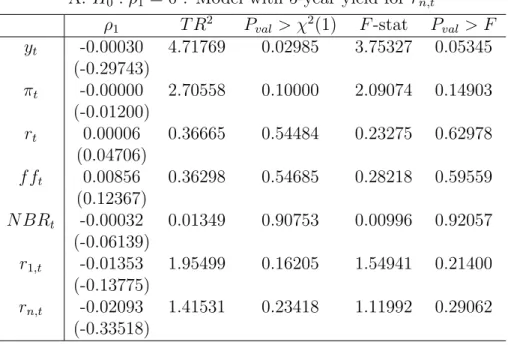
Table 2.3: Autocorrelation test result: H0 :ρ1 = 0

ρ1 t-stat P rob >|t| T R2 P val > χ2(1) F-stat P val > F

yt -0.40762 -1.07138 0.28617 1.49061 0.22212 1.14786 0.28617

πt -0.23201 -0.74327 0.45878 0.74675 0.38751 0.55245 0.45878

wt -0.20131 -0.33436 0.73870 0.24652 0.61954 0.11180 0.73870

f ft 0.38106 1.57984 0.11680 3.23812 0.07194 2.49590 0.11680

N BRt 0.65434 1.37346 0.17219 2.49258 0.11438 1.88640 0.17219

rn,t 0.02832 0.09293 0.92611 0.20576 0.65011 0.00864 0.92611

yt,πt,wt,f ft,N BRt, andrn,trepresent real output, rate of inflation, real wage, federal

funds rate, non-borrowed reserves, and long-term interest rate. 5-year yield series are used for rn,t. The first to third columns present AR(1) coefficients of residuals, their

t-statistics, and theirp-values, respectively. The fourth and fifth columns report theχ2

(39)

Figure 2.1: Autocorrelation functions of VAR residuals I

0

10

20

30 −0.2

0

0.2 y

_t

0

10

20

30 −0.2

0

0.2 π

_t

0

10

20

30 −0.2

0

0.2 w

_t

0

10

20

30 −0.2

0

0.2 ff

_t

0

10

20

30 −0.2

0

0.2 NBR

_t

0

10

20

30 −0.2

0

0.2 r

_n,t

Autocorrelation functions of VAR(K) residual in which quarterly series are used. K = 6 is adopted. yt, πt, wt, f ft, N BRt, and rn,t represent real output, rate of inflation,

(40)

Figure 2.2: Impulse response functions to the federal funds rate shock

0

5

10

15

20 −0.5

0

0.5 RGDP

t

0

5

10

15

20 −0.2

0

0.2 PCE

t

0

5

10

15

20 −0.5

0

0.5 RW

t

0

5

10

15

20 −0.5

0

0.5

1 FF

t

0

5

10

15

20 −2

−1

0

1 NBR

t

0

5

10

15

20 −0.5

0

0.5 YT

t

RGDPt, P CEt, RWt, F Ft, N BRt, and Y Tt stand for real output, rate of inflation, real

wages, federal funds rate, non-borrowed reserves, and 5-year yield as a long rate, respectively. The dash-dot lines represent 95% confidence intervals, and the dotted lines are 68%

confidence intervals using bootstrap Monte-Carlo draws. The sample period is between

(41)

Figure 2.3: Impulse response functions to the federal funds rate shock with commodity price

0

5

10

15

20 −0.5

0

0.5 RGDP

t

0

5

10

15

20 −0.2

0

0.2 PCE

t

0

5

10

15

20 −1

0

1 FF

t

0

5

10

15

20 −2

0

2 NBR

t

0

5

10

15

20 −0.2

0

0.2 RW

t

0

5

10

15

20 −0.2

0

0.2 YT

t

0

5

10

15

20 −2

0

2 PCOM

t

RGDPt, P CEt, RWt, F Ft, N BRt, Y Tt, and P COMt stand for real output, rate of

(42)

Figure 2.4: Impulse response functions of yields to the federal funds rate shock

0

10

20 −0.5

0

0.5

1 1mth

0

10

20 −0.5

0

0.5

1 2mth

0

10

20 −0.5

0

0.5

1 3mth

0

10

20 −0.5

0

0.5

1 4mth

0

10

20 −0.5

0

0.5

1 5mth

0

10

20 −0.5

0

0.5

1 6mth

0

10

20 −0.5

0

0.5

1 1yr

0

10

20 −0.5

0

0.5

1 2yr

0

10

20 −0.5

0

0.5

1 3yr

0

10

20 −0.5

0

0.5

1 4yr

0

10

20 −0.5

0

0.5

1 5yr

0

10

20 −0.5

0

0.5

1 10yr

From the upper left corner to the bottom right, each window represents the impulse response functions of 1- to 6-month and 1- to 10-year maturity yields, respectively. The IRFs are

obtained by switching the long-term bond yield, Y Tt, in the state vector with different

(43)

Figure 2.5: Impulse responses to a term premium shock

0

5

10

15

20 −0.2

0

0.2 RGDP

0

5

10

15

20 −0.2

0

0.2 PCE

0

5

10

15

20 −0.2

0

0.2 RW

0

5

10

15

20 −0.5

0

0.5 FF

0

5

10

15

20 −2

−1

0

1 NBR

0

5

10

15

20 −0.5

0

0.5 YT

A one standard deviation long-term asset market shock is given. RGDPt, P CEt, RWt,

F Ft, N BRt, and Y Tt stand for real output, rate of inflation, real wages, federal funds rate,

non-borrowed reserves, and 5-year yield as a long rate, respectively. The dash-dot lines

(44)

Figure 2.6: Impulse responses to the federal funds rate shock: pre-Volcker period, 1965:Q2-1979:Q3.

0

5

10

15

20 −0.5

0

0.5 RGDP

t

0

5

10

15

20 −0.5

0

0.5 PCE

t

0

5

10

15

20 −0.2

0

0.2 RW

t

0

5

10

15

20 −0.5

0

0.5 FF

t

0

5

10

15

20 −1

0

1 NBR

t

0

5

10

15

20 −0.2

0

0.2 YT

t

RGDPt,P CEt,RWt,F Ft,N BRt, andY Ttstand for real output, rate of inflation, real wages,

(45)

Figure 2.7: Impulse responses to the federal funds rate shock: Volcker-Greenspan pe-riod, 1979:Q4-2005:Q4.

0

5

10

15

20 −0.2

0

0.2 RGDP

t

0

5

10

15

20 −0.1

0

0.1 PCE

t

0

5

10

15

20 −0.5

0

0.5 RW

t

0

5

10

15

20 −0.5

0

0.5 FF

t

0

5

10

15

20 −2

−1

0

1 NBR

t

0

5

10

15

20 −0.2

0

0.2 YT

t

RGDPt,P CEt,RWt,F Ft,N BRt, andY Ttstand for real output, rate of inflation, real wages,

(46)

Figure 2.8: Impulse responses of yields to the federal funds rate shock: pre-Volcker period, 1965:Q2-1979:Q3.

0

10

20 −0.5

0

0.5 1mth

0

10

20 −0.5

0

0.5 2mth

0

10

20 −0.5

0

0.5 3mth

0

10

20 −0.5

0

0.5 4mth

0

10

20 −0.5

0

0.5 5mth

0

10

20 −0.5

0

0.5 6mth

0

10

20 −0.5

0

0.5 1yr

0

10

20 −0.5

0

0.5 2yr

0

10

20 −0.5

0

0.5 3yr

0

10

20 −0.5

0

0.5 4yr

0

10

20 −0.5

0

0.5 5yr

0

10

20 −0.2

0

0.2 10yr

From the upper left corner to the bottom right, each window represents the impulse responses of 1- to 6-month and 1- to 10-year maturity yields, respectively. The IRFs are obtained by

switching the long-term bond yield,Y Tt, in the state vector with different maturity yields one

(47)

Figure 2.9: Impulse responses of yields to the federal funds rate shock: Volcker-Greenspan period, 1979:Q4-2005:Q4.

0

10

20 −0.5

0

0.5

1 1mth

0

10

20 −0.5

0

0.5

1 2mth

0

10

20 −0.5

0

0.5

1 3mth

0

10

20 −0.5

0

0.5

1 4mth

0

10

20 −0.5

0

0.5

1 5mth

0

10

20 −0.5

0

0.5

1 6mth

0

10

20 −0.5

0

0.5

1 1yr

0

10

20 −0.5

0

0.5

1 2yr

0

10

20 −0.5

0

0.5

1 3yr

0

10

20 −0.5

0

0.5

1 4yr

0

10

20 −0.5

0

0.5

1 5yr

0

10

20 −0.5

0

0.5

1 10yr

From the upper left corner to the bottom right, each window represents the impulse responses of 1- to 6-month and 1- to 10-year maturity yields, respectively. The IRFs are obtained

by switching the long-term bond yield, Y Tt, in the state vector with different maturity

(48)

Chapter 3 The Term Premium Response to

Macroeconomic Shocks

My dynamic stochastic general equilibrium (DSGE) model, which will be developed in

the next chapter, incorporates the direct effect of short- and long-term interest rates on

the current and future marginal cost of firms. Since the policy instrument in my model

is a nominal short-term interest rate and the long-term bonds are not redundant assets,

the term structure of interest rates becomes an important monetary policy transmission

channel through which the short-rate monetary policy action has an effect on long rates.

The linearized version of the term structure of interest rates derived in my DSGE model

assumes that the term premium follows an exogenous stochastic white noise process

which implies that the macroeconomic shocks do not affect the term premium, and

the monetary policy shock changes long rates in the direction that the expectations

hypothesis predicts.

The natural question would then be whether the real world data can support

the above relationship between the term premium and the macroeconomic shocks, or

whether the term premium movement with respect to other macroeconomic shocks is

(49)

term premium response implied by the impulse response functions of different maturity

yields to the macroeconomic shocks including the monetary policy shock.

In the next section, I will briefly explain the preliminary information on the yield

curve over the business cycle. In sections 2 and 3, with the method used by Edelberg and

Marshall (1996), I show that the expectations hypothesis does a good job of explaining

the impulse response of different maturity yields to macroeconomic shocks. In section

4, the effects of macro variables on the three factors of the yield curve and on the term

premium will be examined.

3.1 Behavior of the Yield Curve over the Business

Cycle

Figure 3.1 displays the yield curve over the business cycle. For yields data, I used the

CRSP data set from 1965:03 to 2005:12. The yields are 1- to 6-month and 1- to 5-year

maturity yields. The 10-year Treasury constant maturity rate is used for 10-year yield.

The slope is calculated as a difference between 5-year and 1-month zero-coupon bond

yields. The solid line represents the 3-month average slope of yields and the dash-dot

line plots the detrended log real GDP using the HP filter with the quarterly frequency

smoothing parameter of 1600. The vertical dotted lines represent peaks and troughs

announced by NBER.

As Figure 3.1 shows, there exists a negative relationship between the slope of the

yield curve and the output. The correlation coefficient is -0.4347. In particular, the

slope of the yield curve is strictly positive at the bottom of the business cycle. We also

observe a strictly smaller slope at the peak than at the very next trough. According

(50)

cyclical behavior of short-term bond yields due to the Fed’s effort to stimulate the

economy.

3.2 The Term Premium Response to the Monetary

Policy Shock

By changing the short rate, the monetary policy authority affects the long rates through

the policy transmission path known as the term structure of interest rates. I start with

the following well-known term structure equation, which is also derived in my DSGE

model:

rn,t =

1 n

n−1

X

i=0

Etr1,t+i+T Ptn (3.1)

whereT Pn

t denotes the time-varying term premium forn-period bond yield. Equation

(3.1) states that then-period bond yield, rn,t, is determined as the sum of the average

of expected current and future one-period yields up to n-periods and the time-varying

term premium for the n-period bond. Hence, if a policy shock is transmitted through

changing market expectations on future short rates, then the term premium on

long-term bond yields should not be affected by the policy shock.

We can rewrite (3.1) with respect to the term premium for the n-period maturity

bond as the difference between n-period maturity yield and the average of current and

expected one-period maturity yields up to (n−1)-periods given by:

T P_tn=rn,t−

1 n

n−1

X

i=0

Etr1,t+i (3.2)

After taking one-period lead and timetexpectation on both sides of (3.2), the expected

(51)

by the difference between the expected value for timet+ 1n-period maturity yield and

the average of the expected values for one-period maturity yields fromt+ 1 tot+n as

follows

EtT Ptn+1 =Etrn,t+1−

1 n

n

X

i=1

Etr1,t+i (3.3)

The above equation implies that when the state vector in an empirical VAR model

includes one- andn-period maturity yields, we can compute the timet+1 term premium

response for then-period maturity bond to the monetary policy shock as the difference

between the time t+ 1 impulse response function of n-period maturity yield and the

average of impulse response functions of one-period maturity yield from t+ 1 to t+n.

So the state vector in this section includes two different maturity yields together,

one-and n-period maturity yields, in order to calculate the impulse response of the term

premium for the n-period maturity bond.

The state vector is given by

Xt= (IPt, πt, rwt, F Ft, N BRt, r1,t, rn,t)0

In order to take a closer look into the dynamics of yields, monthly series are used to

examine the behavior of the yield curve. Also, the impulse response analysis is

per-formed with variables in levels and the VAR includes a constant vector. By estimating

the system on the original data, without transforming the data into stationary form,1

we can avoid a possible distortion about the long-run property in the system (Sims et

al. 1990, Bagliano and Favero 1998), which could result in a faulty estimation of the

term premium because of the contaminated long-horizon information on the short rate.

1_{Standard ADF tests of a unit root against the alternative of a linear trend and intercept suggest}

The term structure and cost channel effect of monetary policy