tomography images acquired from different imaging systems
Shengnan Liu, Oleh Dzyubachyk, and Jeroen Eggermont
Division of Imaging Processing, Department of Radiology, Leiden University Medical Center, Leiden, 2300 RC, The Netherlands
Shimpei Nakatani
Division of Cardiology, Sakurabashi Watanabe Hospital, Osaka 530-0001, Japan
Boudewijn P. F. Lelieveldt
Division of Imaging Processing, Department of Radiology, Leiden University Medical Center, Leiden, 2300 RC, The Netherlands Intelligent Systems Department, Delft University of Technology, Delft, 2628 CD, The Netherlands
Jouke Dijkstraa)
Division of Imaging Processing, Department of Radiology, Leiden University Medical Center, Leiden, 2300 RC, The Netherlands
(Received 4 December 2017; revised 11 June 2018; accepted for publication 5 July 2018; published 14 August 2018)
Purpose: Intravascular optical coherence tomography (OCT) is widely used for analysis of the coro-nary artery disease. Its high spatial resolution allows for visualization of arterial tissue components in detail. There are different OCT systems on the market, each of which produces data characterized by its own intensity range and distribution. These differences should be taken into account for the devel-opment of image processing algorithms. In order to overcome this difference in the intensity range and distribution, we developed a framework for matching intensities based on the exact histogram matching technique.
Methods: In our method, the key step for using the exact histogram matching is to determine the tar-get histogram. For this, we proposed two schemes: a global scheme that uses a single histogram as the target histogram for all the pullbacks, and a local scheme that selects for each single image a tar-get histogram from a predefined database. These two schemes are compared on a unique dataset con-taining pairs of pullbacks that were acquired shortly after each other with systems from two vendors, St. Jude and Terumo. Pullbacks were aligned according to anatomical landmarks, and a database of matched histogram pairs was created. A leave-one-out cross validation was used to compare perfor-mance of the two schemes. The matching accuracy was evaluated by comparing: (a) histograms using Euclidean (dx2) and Kolmogorov–Smirnov (dKS) distances, and (b) median intensity level within
anatomical regions of interest.
Results: Leave-one-out validation indicated that both matching schemes yield comparably high accuracies across the entire validation dataset. The local scheme outperforms the global scheme with marginally lower dissimilarities at both histogram level and intensity level. High visual similarity was observed when comparing the matched images to their aligned counterparts.
Conclusion: Both local and global schemes are robust and produce accurate intensity matching. While local scheme performs marginally better than the global scheme, it requires a predefined his-togram dataset and is more time consuming. Thus, for offline standardization of the images, the local scheme should be preferred for being more accurate. For online standardization or when another sys-tem is involved, the global scheme can be used as a simple and nearly-as-accurate alternative.© 2018 The Authors. Medical Physics published by Wiley Periodicals, Inc. on behalf of American Associa-tion of Physicists in Medicine.[https://doi.org/10.1002/mp.13103]
Key words: histogram specification, image intensity, intensity standardization, intravascular optical coherence tomography (IVOCT)
1. INTRODUCTION
Cardiovascular diseases (CVDs) are the leading cause of death worldwide.1Introduction of intravascular optical coher-ence tomography (IVOCT) has largely advanced understand-ing and treatment of one of the most common CVDs, the coronary artery disease.2–5Design of IVOCT enables visual-ization of superficial tissue structures of the arteries with res-olution as high as 5–10 lm. The wavelength of its light
source is around 1300 nm, which permits a relatively deep penetration into the vessel wall. Theintravascularterm indi-cates that the images are acquired from the inside of the blood vessel. For current commercial systems, this is achieved by inserting a catheter into the coronary artery, pushing away the blood by injecting a flush media and pulling it back through the lesion location. The catheter has been designed to emit near-infrared light towards the artery wall and to receive the back-propagated light. The received light is recorded as a
4158 Med. Phys. 45 (9), September 2018 0094-2405/2018/45(9)/4158/13
© 2018 The Authors. Medical Physics published by Wiley Periodicals, Inc. on behalf of American Association of Physicists in Medicine. This is an open access article under the terms of the
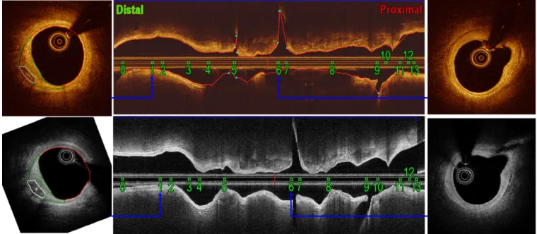
one-dimensional signal (A-line) containing the back-propa-gated intensities ordered by ascending distances to the cathe-ter. By rotating the catheter tip with a constant speed, two-dimensional (2D) images can be generated. Centering at the catheter, each cross-sectional image contains about 500 A-lines from different directions. These A-A-lines are recorded as a raw image in polar coordinates, as shown in Figs.1(b) and 1(e), or transformed into the Cartesian coordinates, as shown in Figs.1(c) and1(f). As the catheter is pulled back at a con-stant speed using a motorized pullback device, a stack of images, referred to as apullbackis acquired.
The use of IVOCT in clinical studies increases exponen-tially.2Because of its high resolution, IVOCT contributed to confirmation of pathological findings on progression of (neo) atherosclerosis by visualizing morphologies like intimal ero-sion, fibrous plaque, calcified nodule, lipid pool, macro-phages distribution, intraluminal thrombus, etc.6–12Attracted by the conspicuous clinical prospects, many efforts were paid to detection and characterization of IVOCT morphologies, such as fibrous, lipid-rich and calcified plaques,13 macrophages distributions,7 thrombus,14 side branches,15,16 struts17–19, and struts embedding20 with image intensities, and/or optical parameters.21,22 However, diversity of IVOCT data can limit comparison of the results, especially when intensity values are used. In particular, there is no consented
standard for the imaging range, unlike, for example, in com-puted tomography (CT), meaning that IVOCT images gener-ated with different commercially available systems are typically characterized by different intensity ranges. The most commonly used commercial systems are the Illumien Optis from St. Jude Medical (St. Paul, MN, USA), which saves the raw data in a 16-bit format, and the Lunawave from Terumo (Tokyo, Japan), which saves the raw data in a 8-bit format.
As a concrete example, the Cartesian images from these two systems are shown in Figs.1(c) and1(f), and their polar coun-terparts are shown in Figs.1(b) and1(e). Images were acquired shortly after each other during the same intervention at the same location inside an artery of one patient. The histograms of the corresponding regions on the IVOCT images acquired by the two systems indicate different intensity ranges within the same tissue type. Furthermore, the different shape of these histograms suggests that relationship of intensities between these two systems is not simply linear. In fact, an exponential relationship has been observed in our previous work.23
Most OCT studies used the same type of IVOCT system to guarantee high reproducibility. On the other hand, doing so limits the scope of developed applications, when the same method is applied to data from another vendor that has differ-ent intensity distribution, repeated validation is required. To improve efficiency of development, images need to be
(a) (b) (c)
(d) (e) (f)
FIG. 1. Histograms (a) of regions delineated in St. Jude polar (b) and Cartesian (c) images. Histograms (d) of regions delineated in Terumo polar (e) and
standardized across devices. Only few papers on this topic have been published in the IVOCT field, whereas several papers on increasing the comparability of ophthalmological OCT images were published. In particular, a normalization approach was proposed for comparing images from two ven-dors.24 This approach involves three steps: density scaling and sampling, noise reduction, and amplitude normalization. It was later improved by integrating virtual averaging.25This A-line normalization approach was shown to reduce the mea-surement difference26and the appearance disparity.27
In this work, we explore the possibility of converting the data between different OCT systems and propose a matching scheme with good generalization and minimal loss of detail. Our pretrained algorithm can also be used for intensity matching when the target data are not given. By doing this, when a method developed for data acquired with system-A needs to be evaluated with data acquired with system-B, we can modify the data from system-B to follow the intensity distribution of system-A, such that the method can be tested on the data from system-B with minimum modification. Such data conversion is referred to as the histogram modifica-tion.28–31The basic histogram matching theory has been pro-posed in the work of Hummel et al.28Since then, this study has been widely used as the fundamental theory in image modification studies at the histogram level. Later, the exact histogram specification (EHS) was proposed as a successful discrete solution to the model in practice.29–31This approach was used to produce comparable measurements in ophthal-mological OCT images generated with low signal strength to that generated with high signal strength32and to compensate light attenuation in confocal microscopy.33
Our main goal in this paper is to propose a framework for matching intensities in OCT images from different vendors using EHS. A straightforward approach would be to match intensities per pullback. We compare thisglobalscheme to a localscheme that takes the local intensity variations into the consideration. All the analyses are conducted with raw polar images, whereas the Cartesian images are only used for the visualization of results. Thein vivopatient data used in this study are unique in the sense that both St. Jude and Terumo pullbacks were specially acquired for this study. A more elab-orate explanation of this is provided further in the manu-script.
The paper is structured as follows. For better understand-ing of the underlyunderstand-ing principles and terminology, we explain both the model and the EHS in Section 2. In Section 3, the data and its processing are described, the distance measures are introduced, and the matching schemes are proposed and validated. Results are reported and discussed in Sections4to 6. Finally, in Section7we draw the conclusions.
2. THEORY AND TERMINOLOGY
Each 2D image can be represented as a matrix I(x,y), which is the discrete subsample of a bounded surface func-tion f(x,y), where{(x,y)|0 ⩽x⩽N,0⩽y⩽ M}. The inten-sity function f(x,y) follows a distribution function Pf(t) that
indicates the chance off(x,y) being less or equal thant. Given two imagesfsPfsðzsÞandftPftðztÞ, the goal of histogram transformation is to search for a mapping T, such that the composition is TfsPftðztÞ. In this work, fs and ft are referred to as the source and the target image, respectively. This search has been formulated by Hummel et al.28 as an optimization problem:
^
T¼arg min
T
Za2
a1
½pTfsðzÞ pftðzÞ 2
dz; (1)
where ½a1;a2 defines the range of image intensities. Here, pX(z) is the probability density function (pdf) of image X,
which is the derivative of the distribution functionPX(z), and
zis intensity level.
A unique monotonic solution of this model was given in Ref.[28]:
~
TðzsÞ ¼Pft1ðPfsðzsÞÞ;pfsðzsÞ[0; for 8zs: (2)
In practice,pXin both source and target spaces is usually
esti-mated as the normalized histogram vector:
pX ¼ fpij
P
pi¼1;i2 f0;. . .;2L01gg, whereL0denotes
the maximum gray level of the images, pi denotes the
fre-quency of the image intensity corresponding to the interval [zi,zi+1). Conventionally, the interval is referred to as a bin;
{zi}are the bin edges; the average of every two adjacent bin
edgesci= (zi+zi+1)/2 is the bin center, andpiis the bin value.
We define the bin edges for theithbin as [ci0.5,ci + 0.5)
in this work.
To ensure that the distribution function PX is
monotoni-cally increasing, the following approximation is used:
Pj¼
cjzj
zjþ1zj
pjþ
Xj1
i¼0
pi: (3)
This approximation is equivalent to interpolating Pj(z) for
z2 ½zj;zjþ1Þ with a piecewise-linear function, the slope of
which ispjand the intercept is
Pj1
i¼0pi. Using this monotonic
approximation, T~ can be estimated with Eq. (2). However, this estimation only shifts bins centers, and splitting of bins is not possible. This becomes especially problematic when the source and the target images are within different intensity range, such as transforming 8-bit images to 16-bit images or the other way around. Since the bins cannot be split, informa-tion can only be retained based on the image that is repre-sented by less bins. Attempts have been made to include local information28 (local mean, entropy, etc.) into the objective function as a“context-aware”term, but doing so introduces more parameters, and the transformed images tend to be blurred.
divided according to any given target histogram. This usually cannot be done by using intensities only, thus auxiliary infor-mation needs to be introduced.
Local means and wavelet coefficients have been reported to be successful source of auxiliary information for achieving strict ordering.30,31 In a more recent study,29 a moderately improved performance in nature images has been reported with a proposed auxiliary term involving three hyperparame-ters. Compared to the other two aforementioned approaches, the local-means approach better copes with noise and involves no hyperparameters, thus it is chosen in this study as the noise level of OCT images is known to be high.
Considering the intensity at each pixel as the first scale of the local mean, for each pixeliwe calculate a vector of multi-scale local means with increasing window size l = [l1(i),
l2(i),. . .,lK(i)], Kbeing the number of scales. Consequently,
all the pixels in the image can be ordered lexicographically with a relational operator defined as
fijjl‘ðiÞ ¼l‘ðjÞ8‘\‘0;l‘0ðiÞ\l‘0ðjÞg: (4)
As result of using this approach, pixels in one image are expected to be ordered strictly by using just a few scales. It was observed thatK= 6 scales are usually enough to arrange all the pixels in a strictly ascending order.30 Once the strict ordering is achieved, the pixels can be easily grouped again following the histogram defined in the target image.
In practice, the EHS is often used to estimate the target image(s) given the source image(s) and the target histogram. In our case, however, the target histogram is unknown and should first be defined using a group of matched source and target images. Thus, our task is twofold: (a) To estimate the target histogram(s) from the matched images, and (b) To apply the estimated histogram(s) to a new source image. The following section describes our method in full detail.
3. MATERIALS AND METHODOLOGY
As it was previously elaborated, the key step for using EHS is to define the target histogram.
3.A. Global and local matching schemes
To determine the target histogram, the most straightfor-ward approach is to use the overall histogram generated with all the images. However, using the global histogram as a ref-erence might result in information loss as some of the less represented tissue structures might get overshadowed in the global histogram. Using local histograms might help resolv-ing this issue.
Therefore, we introduce a Global scheme and a Local scheme for determination of the target histogram. For apply-ing the Local scheme, each pullback is split into smaller sec-tions (our pullback alignment and splitting algorithm is described in the following section). For providing a formal definition, we denote the database of matched histogram pairs as H ¼ fðHk
1;H
k
2Þjk ¼ 1;NHg, whereH1k denotes the
histogram ofkth section in the original space (e.g., St. Jude), Hk
2 denotes its counterpart in the target space (e.g., Terumo), andNHis the size of the database.
For matching a given image with histogramH1, the Global scheme uses one overall histogram as the target histogram, that is,
H2G¼X
NH
k¼1
H2k: (5)
The Local scheme determines the target histogram for each section as the second component of the database entry whose first component is the most similar toH1:
H2L¼Hargmink¼1;NHdðH 1;Hk
1Þ
2 : (6)
Here,d(Hi,Hj) denotes dissimilarity between two histograms
HiandHj. The remainder of this section describes creation of
the histogram database and introduces the dissimilarity mea-sures.
3.B. Data description and alignment
In our case, the target histogram is estimated using a data-set of matched images. As the final goal of this study is to transform OCT images both from intensity space of St. Jude system (St. Jude space) to that of Terumo system (Terumo space) and the other way around, the target histograms in both St. Jude and Terumo spaces need to be determined. To achieve this, eightin vivopullbacks were acquired from left anterior descending artery (LAD) of two different patients, marked asAandB. The data acquisition strictly followed the clinical guideline of Sakurabashi Watanabe Hospital (Osaka, Japan), and the analysts from Leiden University Medical Center (Leiden, The Netherlands) were blinded from all patients’ information. For each patient, IVOCT pullbacks from the same vessel segment were acquired shortly after each other with St. Jude and Terumo systems, before and after the stent implanting procedure. As a result, four pairs of corresponding St. Jude–Terumo pullbacks were made avail-able for the study. The St. Jude pullbacks were acquired at a pullback speed of 36 mm in 180 frames per second with a frame interval of 0.2 mm, and the Terumo pullbacks were acquired at a pullback speed of 40 mm in 158 frames per sec-ond with a frame interval of 0.25 mm. Raw polar images as provided by the vendors are used in this study. St. Jude images are 16-bit “linear” with a transversal pixel size of 0.0050 mm, and Terumo images are 8-bit “log-like” com-pressed with a transversal pixel size of 0.0049 mm.
Compared to the histogram of the entire overlapping part of pullbacks, histograms of smaller sections may preserve more local structural information. Therefore, we further split the overlapping part into small sections using key frames defined by two main types of anatomical landmarks (as shown in Fig.2): the side branches and the tissue types with identical patterns, for exmaple, culprit lesion visible in Fig.1(c) and1(f). For the poststenting pullbacks, the proxi-mal and distal edges of the stent struts are also considered to be crucial landmarks. Key frames were identified indepen-dently by two experienced IVOCT readers, using QCU-CMS (Quantitative Coronary Ultrasound—Clinical Measurement Systems; Leiden University Medical Center, Leiden, The Netherlands), which is the research version of QIVUS (Quan-titative IntraVascular UltraSound; Medis, Leiden, The Netherlands). Only landmarks with consensus were selected.
Even though the catheter is pulled back with a uniform speed, the number of frames within a certain section can be affected by the heartbeat cycle, slight bending of the artery, interaction between the catheter and the artery wall, and so on. Due to this effect, finer splitting or frame-to-frame match-ing is not possible without introducmatch-ing an interpolation error.
Table I gives an overview of the aligned data. Patient-A had no stent planted beforehand, while Patient-B did have one. Hence, the number of frames without stent struts in Patient-B is smaller than in Patient-A. Overall, the pullbacks were aligned with 23 key frames. Within these frames, regions of clinical interest (ROI) were delineated based on their appearance and visible borders according to the consen-sus;11see Fig.1. In total, we have 18 corresponding pairs of sections and 38 ROIs. After correspondence between the sec-tions had been established, the database of matched his-togram pairs was generated using foreground regions bounded by the lumen border and 1 mm behind. This corre-sponds to the depth of 200 pixels in St. Jude polar image and
204 pixels in Terumo polar image. The lumen border is detected by the QCU-CMS software in an automated manner.
3.C. Dissimilarity between histograms
The Euclidean and the Kolmogorov–Smirnov distances are used for comparing two histograms. They are first used in the analysis of the local variations and, after that, for evalua-tion of matching schemes.
For calculating the distances, the histograms are normal-ized to obtain the probability density functions (pdf’s) and the corresponding cumulative density functions (cdf’s). The Euclidean distance for measuring dissimilarity between two pdf’spandqis defined as
dx2ðp;qÞ ¼ ðpqÞ ðpqÞ0; (7)
the discrete approximation of which is equivalent to the objective function in Eq. (1). The Kolmogorov–Smirnov dis-tance measures dissimilarity between the distribution func-tions (also known ascdf’s)PandQ:
dKSðP;QÞ ¼max
i jPiQij: (8)
3.D. Validation
Leave-one-out validation is used to compare the Global and Local schemes. One of the four pullback pairs is left out in turn, and the target histogram is determined with the other three. Consequently, the intensities of the left-out pullback are matched. As part of each leave-one-out experiment, med-ian intensities within each ROI are compared in both target and matched images. The target and matched median values are shown in the scatter plot and compared in the Bland– Alt-man plot. The scatter plot can show whether two groups of
data are linearly related and how much the trend line deviates from the diagonal line, which is the ideal case indicating that two groups of data match perfectly. The Bland–Altman plot shows the average vs the difference of each two compared values, which reveals the difference of two groups of data more explicitly. The mean and the standard deviation values of the difference are also called the systematic difference and the random error. With a properly low random error, the clo-ser the systematic difference to zero level is, the more likely that two groups of data are originating from the same distri-bution. For reference, also the key frames are matched using the target histograms extracted directly from their corre-sponding aligned frames.
4. RESULTS
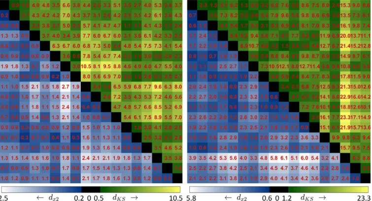
We calculated the distances between all the histograms in two spaces. Figure3gives a general overview of all the dis-similarities. In the scatter plot of distances in Fig. 4, we observed a linear trend and further performed the regression analysis. The statistical results show that the dissimilarities in two spaces are correlated significantly with P < 0.005. This validates the assumption and supports the Local matching scheme.
Results of the leave-one-out validation for both St. Jude-to-Terumo (S?T) and Te-ru-mo-to-St. Jude (T?S) images are reported in Figs.5and6and summarized in TableII. For a section containing 70 images, generating the histograms takes 10 s. For the Local scheme, the time for searching in our database of 34 histograms using our Matlab (MathWorks, R2016a with Statistics and Machine Learning Toolbox) implementation is 1.25 s. Figure5shows the estimated target probability profile (normalized histogram) together with that determined by the aligned data (in red color; will be further referred to as the aligned histogram). The corresponding cumulative probability plots are shown as well. Bothdx2and
dKS are shown as bar charts in Fig.6, and the numbers are
reported in TableII. The distances between matched and ref-erence distributions for both Global and Local schemes are low and robust; see Fig.6and TableII. The average distance
of all four validation experiments (Averin TableII) indicates that, in general, the Local scheme outperforms the Global scheme.
Scatter plots and Bland–Altman plots of the median inten-sities within ROIs are shown in Fig. 7. When comparing intensities in St. Jude space, an increasing trend is observed in the absolute systematic error; see Figs. 7(b), 7(e), 7(h), 7(k). Following the conventional statistical procedure for Bland–Altman analysis,34 the St. Jude intensities were com-pared in the logarithm scale; see Figs. 7(c), 7(f), 7(i), 7(l). Without an obvious trend in Terumo space, the intensities are compared in the linear space; see Fig.7(a),7(d),7(g),7(j).
For the reference matching between the corresponding key frames, the systematic differences are 4.50 for S?T and 0.15 for T?S; see Figs.7(a) and7(c). This difference is the most likely to be caused by the selection of data and is inde-pendent of the scheme used. Using this intrinsic systematic difference as a reference, the absolute systematic differences yielded by the Local scheme are relatively small: 9.67 (S?T) and 0.07 (T?S) for dx2, 7.92 (S?T) and 0.06 (T?S) for
dKS, compared to the Global scheme: 10.26 (S?T), 0.12
(T?S). Taking into consideration the described intrinsic dif-ference, the Local scheme yields absolute values closer to zero for both S?T and T?S matching. All comparisons in Bland–Altman analysis suggest that the Local scheme outper-forms the Global scheme for EHS-based intensity transforma-tion in IVOCT images between St. Jude and Terumo systems. The images matched with the target histogram determined by the Global scheme are shown in Fig.8. The matched images, see Figs. 8(e)–8(h), 8(m)–8(p), and the corresponding aligned images, see Figs.8(a)–8(d),8(i)–8(l), show compara-ble intensity levels in both St. Jude and Terumo spaces.
5. COMPARING ATTENUATION COEFFICIENT VALUES USING BOTH ST. JUDE AND TERUMO IMAGES
One of the postprocessing steps in IVOCT data analysis is the estimation of the attenuation coefficients, which are defined as the distinction rate of light passing through a
TABLEI. Data description.
Patient Treatment
St. Jude Terumo
Landmark Section ROI
PLa(mm) Allb Maxb Minb PLa(mm) Allb Maxb Minb
A Prestenting 108 507 80 10 168 389 88 9 14 13 32
Poststenting 108 69 52 17 147 53 41 12 4 2 4
B Prestenting 75 40 21 19 152 33 19 14 3 2 1
Poststenting 75 12 12 12 111 10 10 10 2 1 1
Total 628 80 10 485 88 9 23 18 38
ROI Adventitia Calcification Fibrous IMLc Lipid Neointima Total
No. 4 11 10 4 3 6 38
aPL: total length of the entire pullback.
volume of tissue with a unit oflm1. It is considered to be a key feature for identification of different tissue types in the arterial wall. In our previous work,35we reported the depth-resolved (DR) estimation using St. Jude images. However, applying this estimation directly to Terumo images results in a different range of values. Therefore, we applied this estima-tion approach to the matched Terumo images (in St. Jude range) to validate the assumption that proposed matching scheme facilitates generalization of the attenuation estimation algorithm developed for St. Jude data to Terumo images. The results described above show comparable performance for both schemes. We further illustrate performance of the
Global scheme for the estimation of attenuation coefficient using the DR method.
The attenuation was estimated both in the matched and original Terumo images. The median values within ROIs were compared to those estimated using St. Jude images. The paired t-test at 5% significance level was used with a null hypothesis that the mean difference between two sets is zero.
Figure 9 shows the Bland–Altman plots of the com-parison of median attenuation coefficient in ROIs in (matched/original) Terumo images and in corresponding ROIs in St. Jude images. In the plot presented in Fig. 9(a), original Terumo images were directly used for
FIG. 3. The distances between all the histograms in the database for St. Jude (left) and Terumo (right) spaces. All the distances were multiplied by a factor of 100
for presentation purposes. In each distance map,dx2anddKSare shown in the lower and upper triangles, respectively. [Color figure can be viewed at wileyonline library.com]
the estimation. Comparing to those estimated using the corresponding St. Jude images, the points are not evenly distributed around the zero-line, and both systematic dif-ference and the range of random error are high. Paired t-test indicates that the mean difference is significantly different from zero with P< 0.001, and the 95% confi-dence interval (CI) is [0.74,1.42]. In Fig. 9(b), the matched Terumo images were used for the estimation. In this case, the difference with the values estimated using the St. Jude images is much smaller, which is indicated by lower systematic difference and random error range,
and the points are more randomly distributed around the zero-line. For this case, paired t-test gives P = 0.320 with a 95% CI of [0.10,0.30].
6. DISCUSSION
Clinical significance of IVOCT structures has been reported extensively in clinical research. The use of IVOCT for the analysis of CADs grows exponentially. For more effi-cient analysis with minimum manual intervention, automated methods for tissue quantification, characterization, and
FIG. 5. The aligned and trained probability and the cumulative probability distributions for leaving the 1st (a), the 2nd (b), the 3rd (c), and the 4th (d) pullback
classification are needed. However, a lack of standardized image intensities can increase the difficulty of designing algorithms or restrict the possibility of generalization of algo-rithms developed for one specific imaging system. Therefore, standardizing image intensity is a crucial processing step to speed up the development and validation of methods for intravascular tissue analysis.
This study aims at exploring a proper scheme to match IVOCT image intensities with the local-mean EHS technique. In our case, the most essential step is to determine the target histogram. Preliminary statistical analysis suggests that dis-tances in both spaces are significantly correlated. Based on this analysis, we propose a Local matching scheme and
compare it with the Global scheme. Target histograms deter-mined with both schemes turned out to be successful in matching IVOCT intensities at relatively low cost. In this, Local scheme marginally outperforms the Global scheme, which is in line with the results of our preliminary statistical analysis. Moreover, the attenuation estimation experiment presented in Section5illustrates benefits of using the Global scheme in practice by showing that it, in particular, largely improves the compatibility of the estimated attenuation coef-ficient across vendors.
Significant variation in the histograms of different sections is caused by many reasons, the difference in tissue composi-tion being the major factor. As it has been reported in Ref.
FIG. 6. The bar chart of the distances for leave-one-out experiment for matching St. Jude to Terumo (S?T) space and Terumo to St. Jude (T?S) space.
“Pb”=“pullback”. [Color figure can be viewed at wileyonlinelibrary.com]
TABLEII. Results of leave-one-out cross validation.
S?T T?S
Pb1 Pb2 Pb3 Pb4 Avera Pb1 Pb2 Pb3 Pb4 Avera
dx2 Global 0.0248 0.0135 0.0381 0.0241 0.0251 0.0058 0.0046 0.0110 0.0090 0.0076
Local 0.0192 0.0141 0.0231 0.0091 0.0164 0.0069 0.0053 0.0042 0.0049 0.0053
dKS Global 0.0994 0.0593 0.1398 0.0711 0.0924 0.0252 0.0179 0.0303 0.0273 0.0252
Local 0.1022 0.0724 0.1110 0.0347 0.0801 0.0276 0.0137 0.0246 0.0183 0.0210
a
[5], tissue types are mainly visually assessed by recognizing bright speckle, presence of following shadow, sharpness of border, etc. Quantitative results confirm that these image structures yield variations in the histogram. Our previous study36 demonstrated that image intensities can also be affected by position of the catheter. This effect can cause a large variation in the distances and can, thus, explain the low R2in the reported statistical analysis.
The Bland–Altman analysis shows a systematic difference in median intensities within selected regions of interest, even when the exact histogram is specified using the matched key frames. This intrinsic variation may be caused by many fac-tors, such as the data alignment bias, intrinsic difference in systems for data acquisition, etc. Although this difference is relatively low, it should be accounted for in future applica-tions of this method.
For clinical application, both schemes can also be easily embedded as an independent function for automated intensity standardization. For the global scheme, the target histogram needs to be saved within the program. During calculation, this target histogram is loaded and used in EHS. For the local scheme, the database of histogram pairs needs to be saved. During calculation, the target his-togram needs to be searched in the database and then it is used in EHS. Furthermore, the proposed experimental setup is not limited to the two considered IVOCT systems and can be used to standardize image intensities between other OCT systems or even for other modalities, for exam-ple, MRI. Matching images to St. Jude or Terumo images can also further speed up the validation of newly devel-oped IVOCT systems. As long as the order of intensities of different structures in both systems is consistent, strict
ordering can be applied to insure that the exact histogram can be specified.
In this work, we developed and presented a framework for minimizing intensity variation between two different IVOCT systems. At the same time, there might be variations caused by differences between systems from the same vendor, differ-ences between catheters for the same imaging machine, and even differences in the pullbacks acquired using the same hardware and catheter. Since the images were calibrated by design during the acquisition, we expect these variations to be small.
Bare metal stents (BMS) were implanted in two out of the four pullbacks used in this particular study. Due to their high light reflectance, the BMS struts appear on the images as sat-urated bright spots with dark shadows behind them. They dis-turb the intensity distribution. Since this work mainly focused on matching images of the arterial tissue, images with stent struts were deliberately excluded from the analysis.
6.A. Limitation
The data used in this study are specially generated for con-struction of this intensity matching framework. Performing (virtually) simultaneous acquisition with two IVOCT systems is not done in clinical practice. Therefore, the amount of data used in this study is limited, which is a major limitation of this work. However, these data are unique and more represen-tative for the analysis on intensity matching thanex vivoand animal data. Furthermore, results of leave-one-out validation show reasonable robustness through pullbacks and patients. At the same time, we acknowledge that extending the his-togram database might potentially improve the hishis-togram
FIG. 7. Scatter and Bland–Altman plots for comparing the median intensities within ROIs in target and matched frames (n=38). Reference intensities, matched
according to the aligned key frames (a,c), compared to that matched with the Global scheme (d,f), the Local scheme withdx2(g,i) and the Local scheme withdKS (j,l). In the scatter plots, the regression line is shown as the solid line and the dashed line indicates they=xline. In the Bland–Altman plots, thex-axis and the
matching as using a larger database will most likely lead to more reliable estimation of the target histograms for both Global and Local schemes.
6.B. Future work
This histogram matching scheme will be used for stan-dardization of IVOCT image intensities as a crucial first step for further quantification. Our future work will focus on comparing the outcome of existing quantification
methods, such as attenuation estimation, quantification of the degradation of bioresolvable struts and differentiation of neointima, to data acquired by different IVOCT sys-tems.
Once the matching framework is extensively validated, this approach can be routinely used as a preprocessing step for data standardization. The standardized images can be used for the development of universal algorithms for segmentation (of, for example, fibrous cap of TCFAs) or tissue analysis (e.g., for estimation of attenuation coefficients).
(a)
(b)
(c)
(d)
(e)
(f)
(g)
(h)
(i)
(j)
(k)
(l)
(m)
(n)
(o)
(p)
In this study, we did not include the stented segments of the pullbacks due to the high reflectance of the metallic struts. However, for future work the database could be extended with the stented segments of the pullbacks by excluding individual strut points and their shadows from the images (rather than excluding the entire frame).
7. CONCLUSION
In this work, we presented our contribution to the construction of an intensity standardization framework for IVOCT images. We further contribute to the valida-tion of two proposed schemes in the framework with data acquired by two of the most commonly used IVOCT systems in clinical research. Both local and glo-bal schemes are robust and produce accurate intensity matching. While local scheme performs marginally better than the global scheme, it requires a predefined his-togram dataset and is more time consuming. Thus, for offline standardization of the images, the local scheme should be preferred for being more accurate. For online standardization or when another system is involved, the global scheme can be used as a simple and nearly-as-accurate alternative.
ACKNOWLEDGMENTS
This research was supported by the China Scholarship Council (No. 201206130062).
CONFLICTS OF INTEREST
The authors have no conflicts to disclose.
a)Author to whom correspondence should be addressed. Electronic mail:
J.Dijkstra@lumc.nl.
REFERENCES
1. Mozaffarian D, Benjamin EJ, Go AS, et al. Heart disease and stroke statistics 2016 update.Circulation2016;133:e38–360.
2. Bouma BE, Villiger M, Otsuka K, Oh W-Y. Intravascular optical coher-ence tomography [invited].Biomed Opt Express. 2017;8:2660–2686. 3. Prati F, Guagliumi G, Mintz GS, et al. Expert review document part 2:
methodology, terminology and clinical applications of optical coherence tomography for the assessment of interventional procedures.Eur Heart J.2012;33:2513–2520.
4. Prati F, Regar E, Mintz GS, et al. Expert review document on methodol-ogy, terminolmethodol-ogy, and clinical applications of optical coherence tomog-raphy: physical principles, methodology of image acquisition, and clinical application for assessment of coronary arteries and atherosclero-sis.Eur Heart J.2010;31:401–415.
5. Tearney GJ, Regar E, Akasaka T, et al. Consensus standards for acquisi-tion, measurement, and reporting of intravascular optical coherence tomography studies: a report from the international working group for intravascular optical coherence tomography standardization and valida-tion.J Am Coll Cardiol.2012;59:1058–1072.
6. Ino Y, Kubo T, Tanaka A, et al. Difference of culprit lesion morpholo-gies between ST-segment elevation myocardial infarction and non-ST-segment elevation acute coronary syndrome. JACC Cardiovasc Interv.
2011;4:76–82.
7. MacNeill BD, Jang IK, Bouma BE, et al. Focal and multi-focal plaque macrophage distributions in patients with acute and stable presentations of coronary artery disease.J Am Coll Cardiol.2004;44:972–979. 8. Tanaka A, Imanishi T, Kitabata H, et al. Morphology of
exertion-triggered plaque rupture in patients with acute coronary syndrome: an optical coherence tomography study. Circulation. 2008;118:2368– 2373.
9. Tanimoto T, Imanishi T, Tanaka A, et al. Various types of plaque disrup-tion in culprit coronary artery visualized by optical coherence tomogra-phy in a patient with unstable angina.Circ J. 2009;73:187–189. 10. Taruya A, Tanaka A, Nishiguchi T, et al. Vasa vasorum restructuring in
human atherosclerotic plaque vulnerability: a clinical optical coherence tomography study.J Am Coll Cardiol. 2015;65:2469–2477.
11. Tian J, Hou J, Xing L, et al. Significance of intraplaque neovasculariza-tion for vulnerability: Optical coherence tomography study.J Am Coll Cardiol.2012;59:E1439.
12. Uemura S, Ishigami KI, Soeda T, et al. Thin-cap fibroatheroma and microchannel findings in optical coherence tomography correlate with subsequent progression of coronary atheromatous plaques.Eur Heart J.
2012;33:78–85.
13. Yabushita H, Bouma BE, Houser SL, et al. Characterization of human atherosclerosis by optical coherence tomography. Circulation. 2002;106:1640–1645.
14. Kume T, Akasaka T, Kawamoto T, et al. Assessment of coronary arterial thrombus by optical coherence tomography. Am J Cardiol.
2006;97:1713–7.
15. Karanasos A, Tu S, van Ditzhuijzen NS, et al. A novel method to assess coronary artery bifurcations by oct: cut-plane analysis for side-branch ostial assessment froma main-vessel pullback.Eur Heart J Cardiovasc Imaging2015;16:177–189.
16. Cao Y, Jin Q, Chen Y, et al. Automatic identification of side branch and main vascular measurements in intravascular optical coherence tomogra-phy images. In:2017 IEEE 14th International Symposium on Biomedical Imaging (ISBI 2017). Melbourne: VIC; 2017:608–611.
17. Adriaenssens T, Ughi GJ, Dubois C, et al. Automated detection and quantification of clusters of malapposed and uncovered intracoronary stent struts assessed with optical coherence tomography.Int J Cardio-vasc Imaging. 2014;30:839–848.
18. Wang A, Eggermont J, Dekker N, et al. Automatic stent strut detection in intravascular optical coherence tomographic pullback runs.Int J Car-diovasc Imaging. 2013;29:29–38.
19. Wang Z, Jenkins MW, Linderman GC, et al. 3-d stent detection in intravascular OCT using a bayesian network and graph search. IEEE Trans Med Imaging. 2015;34:1549–1561.
20. Sotomi Y, Tateishi H, Suwannasom P, et al. Quantitative assessment of the stent/scaffold strut embedment analysis by optical coherence tomog-raphy.Int J Cardiovasc Imaging. 2016;32:871–883.
21. Ughi GJ, Adriaenssens T, Sinnaeve P, Desmet W, D’hooge J. Automated tissue characterization of in vivo atherosclerotic plaques by intravascular optical coherence tomography images.Biomed Opt Expr. 2013;4:1014– 1030.
22. van Soest G, Koljenovic S, Bouma BE, et al. Atherosclerotic tissue char-acterization in vivo by optical coherence tomography attenuation imag-ing.J Biomed Opt.2010;15:11105.
23. Liu S, Eggermont J, Nakatani S, Lelieveldt BPF, Dijkstra J. Light inten-sity matching between different intravascular optical coherence tomogra-phy systems.Proc SPIE. 2016a;9689:96893D–96897D.
24. Chen C-L, Ishikawa H, Wollstein G, et al. Individual a-scan signal nor-malization between two spectral domain optical coherence tomography devices.Invest Ophthalmol Vis Sci.2013b;54:3463–3471.
25. Chen C-L, Ishikawa H, Wollstein G, Bilonick RA, Kagemann L, Schu-man JS. Virtual averaging making nonframe-averaged optical coherence tomography images comparable to frame-averaged images.Transl Vis Sci Technol.2016;5:1.
26. Chen C-L, Ishikawa H, Ling Y, et al. Signal normalization reduces sys-tematic measurement differences between spectral-domain optical coher-ence tomography devices.Invest Ophthalmol Vis Sci.2013a;54:7317– 7322.
27. Chen C-L, Ishikawa H, Wollstein G, Bilonick RA, Kagemann L, Schu-man JS. Signal normalization reduces image appearance disparity among multiple optical coherence tomography devices.Transl Vis Sci Technol.
2017;6:13.
28. Hummel RA. Histogram modification techniques.Comput Graph Image Process. 1975;4:209–224.
29. Nikolova M, Wen Y-W, Chan R. Exact histogram specification for digi-tal images using a variational approach. J Math Imaging Vis.
2013;46:309–325.
30. Coltuc D, Bolon P, Chassery JM. Exact histogram specification.IEEE Trans Image Process. 2006;15:1143–1152.
31. Wan Y, Shi D. Joint exact histogram specification and image enhance-ment through the wavelet transform. IEEE Trans Image Process. 2007;16:2245–2250.
32. Chen C-L, Ishikawa H, Wollstein G, et al. Histogram matching extends acceptable signal strength range on optical coherence tomography images.Invest Ophthalmol Vis Sci.2015;56:3810–3819.
33. Stanciu SG, Stanciu GA, Coltuc D. Automated compensation of light attenuation in confocal microscopy by exact histogram specification.
Microsc Res Tech.2010;73:165–175.
34. Euser AM, Dekker FW, le Cessie S. A practical approach to Bland-Alt-man plots and variation coefficients for log transformed variables.J Clin Epidemiol.2008;61:978–982.
35. Liu S, Sotomi Y, Eggermont J, et al. Tissue characterization with depth-resolved attenuation coefficient and backscatter term in intravascular optical coherence tomography images.J Biomed Opt.2017;22:1–16. 36. Liu S, Eggermont J, Wolterbeek R, et al. Analysis and compensation for