umi-unc-1027.pdf

(1)

Bayesian Methods for Highly Correlated Exposures:

an Application to Tap Water Disinfection

By-Products and Spontaneous Abortion

by

Richard F. MacLehose

A dissertation submitted to the faculty of the University of North Carolina at Chapel Hill in partial fulfillment of the requirements for the degree of Doctor of Philosophy in the Department of Epidemiology.

Chapel Hill 2006

Approved by:

Dr. Jay Kaufman, Advisor

Dr. David B. Dunson, Reader

Dr. Katherine E. Hartmann, Reader

Dr. Amy H. Herring, Reader

Dr. Charles Poole, Reader

(2)

c

° 2006

(3)

ABSTRACT

RICHARD F. MACLEHOSE: Bayesian Methods for Highly Correlated Exposures: an Application to Tap Water Disinfection By-Products and

Spontaneous Abortion.

(Under the direction of Dr. Jay Kaufman.)

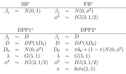
Highly correlated exposures are common in epidemiology. However, standard max-imum likelihood techniques frequently fail to provide reliable estimates in the pres-ence of highly correlated exposures. As a result, hierarchical regression methods are increasingly being used. Hierarchical regression places a prior distribution on the exposure-specific regression coefficients in order to stabilize estimates and incorporate prior knowledge. We examine three types of hierarchical models: semi-Bayes, fully-Bayes, and Dirichlet Process Priors. In the semi-Bayes approach, the prior mean and variance are treated as fixed constants chosen by the epidemiologist. An alternative is the fully-Bayes approach that places hyperprior distributions on the mean and variance of the prior distribution to allow the data to inform about their values. Both of these approaches rely on a parametric specification for the exposure-specific coefficients. As a more flexible nonparametric option, one can use a Dirichlet process prior which also serves to cluster exposures into groups, effectively reducing dimensionality. We examine the properties of these three models and compare their mean squared error in simulated datasets.

(4)

(5)

ACKNOWLEDGMENTS

This dissertation contains a great deal of work that I could not have accomplished without the help of many people. I am grateful to the help of my entire dissertation committee, from whom I have learned a great deal and who have suffered my frequent topic changes with great patience. My advisor and committee chair, Jay Kaufman, has been selfless with his time and advice. I have been the recipient of his tremendous knowledge of epidemiologic methods since I entered the department. This dissertation would not have been possible without the support of David Dunson, whose knowledge of biostatistics is only equalled by his willingness to share it. He has been a source of wonderful ideas and tremendous support.

(6)

LIST OF FIGURES

1.1 Directed acyclic graph depicting the relation between disinfection by-products and spontaneous abortion. . . 11 1.2 Distribution of MLE and ridge regression coefficients. . . 12 2.1 Histogram of 1000 samples drawn from DP(λ= 50, G0 =N(0,1)). . . . 34 2.2 Histogram of 1000 samples drawn from DP(λ= 5, G0 =N(0,1)). . . . 35 3.1 DAG for correlated exposure variables. . . 55 3.2 Distribution of SB and ML estimators. . . 56 3.3 Probability of finding at least one false positive result in SB models as

the number of covariates increases. . . 58 3.4 Distribution of β₁f b and φ2 _{in FB analysis with} _α

1 = 1 and α2 = 1. . . . 60 3.5 Mean squared error of parameter estimates under different

combina-tions of coefficient effects and correlation. The parameter estimates from the 5 models (MLE, SB, FB, DPP, DPP with selection component) are grouped in order within each of the 10 coefficients. . . 62 3.6 Coverage probability for credible intervals by prior mean and variance. 65 4.1 Convergence of the 4 hierarchical models for the effect of the 4th_quartile

of Cl2AA (vs the 1st quartile) on SAB. . . 79 4.2 Posterior distribution of the effect of the highest quartile of CL2AA (vs.

(10)

LIST OF TABLES

3.1 Hierarchical models used in analysis of simulated data. . . 51

3.2 Hierarchical models used to analyze Agricultural Health Study data on herbicides and macular degeneration. . . 52

3.3 Estimated effects of exposure to herbicides on retinal degeneration among the wives of pesticide applicators, Agricultural Health Study, North Car-olina and Iowa, 1993-1997. . . 53

4.1 Bayesian hierarchical models used in RFTS Analysis. . . 82

4.2 Adjusted odds ratios for the association between constituent DBPs and SAB estimated from RFTS. . . 83

4.3 Sensitivity analysis for semi-Bayes model. . . 89

4.4 Sensitivity analysis for fully-Bayes model (prior mean=1.0). . . 92

4.7 Sensitivity analysis for DPP1 model. . . 104

(11)

CHAPTER 1 BACKGROUND

1.1 Spontaneous Abortion

Spontaneous abortion is defined as a pregnancy loss prior to 20 weeks of completed gestation. The exact risk of spontaneous abortion is unknown, largely because of dif-ficultly in detecting early pregnancy. However, spontaneous abortion is well known to be a common occurrence in pregnancy, with over 30% of all pregnancies ending in a loss and roughly 20% of all pregnancies ending in loss before they are clinically de-tectable.(Wilcox et al., 1988) Risk of spontaneous abortion remains high (roughly 1.0% each week) through the 12th _{week of gestation and then rapidly declines.(Goldhaber} and Fireman, 1991)

(12)

1986; Wen et al., 2001)

1.2 Disinfection Process

One of the first uses of chlorine as a disinfectant was by Semmelweis who reduced the transmission rate of puerperal fever by hand-washing with chlorine. Following John Snow’s research on the cause of cholera in London in 1850, interest was raised in finding ways to provide safe, uncontaminated drinking water. Indeed, Snow himself added chlorine to the Broad street pump in an effort to eliminate cholera. Thirty-one years later, Koch formally demonstrated the anti-microbial properties of hypochlorite. In 1902, the public water supplies in Middelkerke, Belgium began to be routinely treated with chlorine. The first municipality to adopt chlorination in the United States was Jersey City, New Jersey in 1908.(White, 1999) Since then, routine disinfection of water has become standard, although the type of disinfection varies among municipalities.

(13)

chem-ical composition of ozone, however, makes it very unstable and insoluble in water and therefore ozone provides little or no continued disinfection after the water leaves the treatment facility. To prevent contamination of the newly treated water while it flows through the pipes, water treatment facilities commonly put a small amount of chlorine (again, either free chlorine or chloramines) into the water supply before it leaves the facility. In equal concentrations, chloramines (a mixture of NH2Cl, NHCl2, and NCl3) are less effective in killing bacteria and viruses but also less likely to combine with organic material and form disinfection by-products than free chlorine, which has led to its widespread use.(Hoff, 1986) Finally, in order to remove any residual biotic growth on pipes downstream of the treatment facility, many public water systems introduce higher concentrations of free chlorine for a short time each year.

The use of disinfectants in the water supply has led to dramatic decreases in the incidence of typhoid, paratyphoid, cholera, legionnaire’s disease, and dysentery. How-ever, the addition of these disinfectants has not been without controversy: chlorination of water supplies has led to many law suits, which ended in the courts upholding the rights of the state to disinfect the water supply by routine use of chlorination in order to better protect the public health.

1.3 Disinfection By-products

(14)

(Cl3AA), bromodichloroacetic acid (BrCl2AA), dibromochloroacetic acid (Br2ClAA), and tribromoacetic acid (Br3AA).

Following the discovery of disinfection by-products in the water supply, epidemio-logic studies began to examine potential adverse outcomes associated with disinfection by-products. These studies initially focused on the effect of disinfection by-products (particularly THMs) on different types of cancer. Increased risk of bladder cancer and to a lesser extent rectal and colon cancer have been associated with increased consump-tion of disinfecconsump-tion by-products.(Crump and Guess, 1982; Mughal, 1992; Villanueva et al., 2004) Other studies of disinfection by-products and reproductive health have linked THM4, chloroform and bromodichloromethane to intrauterine death, stillbirth and miscarriage.(Aschengrau et al., 1989; Bove et al., 1995; Dodds et al., 2004, 1999; King et al., 2000; Savitz et al., 1995)

1.4 Animal Studies

(15)

1.5 Previous Research on Disinfection By-products

and Spontaneous Abortion

(16)

drinkers relative to bottled-water drinkers (RR=2.2, 95%CI (1.3, 3.6)). (Aschengrau et al., 1989)

All of these studies are limited in their exposure assessment; none attempted to measure the amount of disinfection by-products in the water, with most relying simply on consumption of tap-water as a surrogate. In 1995, Savitz et al. used quarterly averages of THM levels to measure the effect of THM consumption on spontaneous abortion in a case-control study in central North Carolina. They found a modest in-crease in the odds of spontaneous abortion (OR=1.7; 95% CI: 1.1, 2.7) for each 50 part per billion unit increase in THM level.(Savitz et al., 1995) In a prospective cohort study, Swan et al found an increased risk of spontaneous abortion among women who drank more than 5 glasses of tap water per day (OR=2.2, 95%CI: 1.2-3.9), however this result was only found in one region of their study. Waller et al. furthered these findings by assigning a THM level to each woman in the study, equal to the reported THM level from each woman’s water service provider. They found that of the four tri-halomethanes, CHBrCl2 was associated with an increased risk of spontaneous abortion (OR=2.0, 95%CI: 1.2-3.5).(Waller et al., 1998) Waller et al. and a previous analysis of Right from the Start by Savitz et al. remain the only study that has examined constituent disinfection by-products rather than the aggregate measures of THM or glasses of water consumed.(Savitz et al., 2005; Waller et al., 1998)

(17)

1.6 Highly Correlated Data in Epidemiology

Because of the high proportion of pregnant women who are exposed to disinfection by-products through tapwater, any effect of disinfection by-products on spontaneous abortion could have enormous public health implications. Unfortunately, efforts to measure the effect of the 13 constituent disinfection by-products (4 THMs and 9 HAAs) on spontaneous abortion are hindered by the high correlation between the disinfection by-products. The amount of chlorine in the disinfection process, the amount of organic matter in the water supply, and the amount of bromide in the water supply all effect the concentration of the 13 disinfection by-products. These common latent factors not only cause a high correlation but also serve to confound the effect of any one of the 13 constituent disinfection by-products unless the remaining 12 are controlled for (Figure 1.1). Unfortunately, common approaches to controlling confounding, such as maximum likelihood regression, perform poorly in precisely this setting.

Highly correlated exposure data frequently arise when the multiple exposures are caused by a single, but frequently latent, factor. Such problems with high correlation are common in epidemiology. For instance, in nutritional epidemiology vitamins and nutrient levels will commonly be highly correlated because of food preferences by indi-viduals. In epidemiologic studies of pesticides, the exposure to certain chemicals may be correlated because they are common to multiple pesticides. Occupational exposures may also be highly correlated since a person’s occupation typically dictates exposure to multiple chemicals.

1.7 Common Methods for Correlated Data

(18)

an effect on spontaneous abortion and all are caused by a common unmeasured factor, then any given exposure is confounded by the remaining 12. A regression model that estimates the effect of only one disinfection by-product, while excluding the other 12, will therefore produce confounded estimates of effect. An alternative approach is to col-lapse the correlated exposure variables into a summary statistic, such as the mean or a weighted average. Such an approach, while generally allowing the maximum likelihood logistic regression to converge, is unappealing since it makes interpretation difficult and can mask important individual effects in the data. For instance, if only one of the 13 disinfection by-products has an effect, an exposure metric that is a weighted average of all 13 disinfection by-products will show a diluted, and possibly difficult to detect, effect. Previous analyses of disinfection by-product data have generally adopted this approach, collapsing the constituent disinfection by-products into categories such as THMs or HAAs.

Problems with collinearity have motivated a number of alternatives to maximum likelihood estimation. An early approach was ridge regression, which modifies max-imum likelihood estimation by including a penalty, k, for large negative or positive values of the regression coefficients.(Hoerl and Kennard, 1970a,b) This penalty can be shown to correspond to the inverse of the variance of a normal prior distribution on the regression coefficients, so that ridge regression is a type of Bayesian estimator.(Lindley and Smith, 1972) When k = 0, there is an infinite prior variance (no penalty) and

βRG ₌ _βM LE _{(RG=ridge regression estimate, MLE=maximum likelihood estimate);} however with k > 0, ridge regression coefficients will be shrunk toward zero and have smaller variance than the MLEs.(Hoerl and Kennard, 1970b) As illustration, consider a normal linear regression

E(Yi|xi1, xi2) =β1xi1+β2xi2 (1.1)

(19)

results from this example are indicative of the general improved performance for ridge regression relative to MLE: while MLEs are asymptotically unbiased, their variance can be enormous and their mean squared error (MSE) is worse than the MSE for ridge regression estimates, which are slightly biased but have a greatly decreased MSE.(Hoerl and Kennard, 1970b; Strawderman, 1978)

1.8 Hierarchical Models

Although ridge regression has only seen limited use in epidemiology, it represents a special case of a broader type of model that has seen some use: hierarchical models. Hierarchical models are those that define model parameters in an ordered structure. For instance, a basic linear regression such as that in equation 1.1 models the random variable yi conditional on parameters β1 and β2. These parameters can in turn be modeled conditional on other parameters (called hyperparameters), for example βi ∼

N(µ, φ2_{), where} _N _{is a normal distribution with mean} _µ_{and variance} _φ2_{. In the ridge} regression example, µ = 0 and φ2 _{= 1}_/k_{. Ridge regression stops at this level of the} hierarchy but the hyperparameters (µ and φ2_{) can in turn be modeled conditional on} still other parameters, for example: µ ∼ N(ψ, ζ) and φ2 _∼ _IG₍_α

1, α2), where IG is the inverse gamma distribution. A parameter, conditional on the parameters one level above it in the hierarchy, is independent of other parameters. For instance, after accounting forβ1 andβ2, the parameters µ, φ2, α1 andα2 contain no information about

yi.

(20)

size.

Hierarchical models are becoming more common in epidemiology. They have seen use investigating the association between occupational exposures and neuroblastoma, between pesticide exposure and neuroblastoma, between genotypes and bladder cancer, and between nutrition and breast cancer.(De Roos et al., 2001; Hung et al., 2004; Kirrane et al., 2005; Witte et al., 1994) However, these models all represent the most basic Bayesian hierarchical model: one with only two levels. Such models have been referred to as semi-Bayes models.(Greenland, 1992, 1993, 1994; Greenland and Poole, 1994) However, the hierarchical framework lends itself to being easily expanded past two levels. Specifying additional levels can allow for large gains in parameter precision and, paradoxically, can limit the reliance of model estimates on user specified parameters (such as µand φ in the semi-Bayes model).

1.9 Summary

(21)

FIGURE

1.1:

Directed

acyclic

graph

depicting

the

relation

b

et

w

een

disinfection

by-pro

ducts

and

sp

on

taneous

ab

(22)

FIGURE

1.2:

Distribution

of

MLE

and

ridge

regression

co

efficien

(23)

CHAPTER 2 METHODS

2.1 Overview of Right From the Start

(24)

to move out of the area before the end of the study 7) were able to read and write in English or Spanish and 8) if they had not yet conceived, they could not have been trying to conceive for greater than 6 months. Enrollment in site 1 began in 2001; sites 2 and 3 began enrollment in 2002. Women were recruited into the study through promotional information in public and private obstetric practices, community-based recruitment (child-care facilities, churches, fitness clubs, etc), and through local drug stores (where invitations to join the study were available near pregnancy test kits). After women contacted the study, an initial screening interview was performed to ensure that they met eligibility requirements.

2.1.1 Data Collection

If a woman met the eligibility criteria, informed consent was obtained and a base-line interview was conducted to collect pertinent information including: age, ethnicity, caffeine consumption, education, marital status, income, smoking status, alcohol use during pregnancy, previous pregnancy history, menstrual history, diabetes history, vi-tamin use and water consumption. Following the baseline interview, study participants were scheduled for an ultrasound that occurred between 6 2/7 and 7 5/7 weeks of gestation but no later than 14 0/7 weeks. The first trimester ultrasound was used to accurately determine gestational age of the fetus, fibroid status of the mother, and other physiologic information. A follow-up interview with all participants occurred between the 20th and 25th week of gestation and was used to ascertain water use, pregnancy related symptoms, and prenatal care. Following the end of the pregnancy, trained chart reviewers abstracted data from each participant’s medical records for outcome ascertainment as well as additional medical information.

2.1.2 Water Sampling

(25)

as the secondary disinfectant. Chloramine is less likely to combine with organic mate-rial and form disinfection by-products outside of the water treatment facility, ensuring a relatively constant concentration disinfection by-products throughout these to cities. However, for a period of 2 weeks in site 3 and one month in site 1, free chlorine was added to disinfect the pipes in the water system. The highly reactive chlorine (which makes it a particularly good disinfectant) readily combined with organic molecules, pro-ducing heterogeneity in levels of disinfection by-products throughout the water system. During the months of free chlorine use in these two cities, samples were drawn from 10 locations throughout each water distribution system, in order to reflect the poten-tial heterogeneity of disinfection by-product concentrations. Additionally, periodically during the study, samples were drawn at locations throughout the water distribution system in order to ensure that disinfection by-product measurements calculated from samples at the point of entry correlated with measurements throughout the distribution system. THM samples were analyzed within 2 weeks of collection and HAA samples within 3 weeks. EPA standard Method 551.1 was used to analyze the concentration of THM levels in water samples and EPA standard Method 552.2 was used to analyze HAA concentrations.(EPA, 1995a,b) All samples were analyzed with a 5890 series II gas chromatograph (Agilent Technologies, Palo Alto, CA) equipped with an electron capture detector. A carrier gas of Ultra High Purity helium and a make-up gas of Ultra High Purity Nitrogen were used.

2.2 Overview of Analysis

(26)

four hierarchical models are described in detail below and in Chapter 3.

2.3 Bayesian Analysis

The vast majority of analytic techniques employed in epidemiology are frequentist and rely on hypothetical repeated sampling of some super-population for their interpreta-tion. While there are many reasons to object to frequentist inference (such as violation of the likelihood principle), there are three very pragmatic reasons why epidemiolo-gists should be skeptical of a strictly frequentist approach to data analysis.(Lindley and Phillips, 1976) First, frequentist analyses, by relying on repeated sampling, often give obtuse answers to questions. For instance, the interpretation of a 95% confidence interval for an OR is that under a very large number of samples generated in precisely the same way, 95% of the constructed intervals will contain the true OR. In most epi-demiologic settings such an interval has little use: the constructed interval in one study either does or does not contain the true value and the 95% confidence interval does nothing to inform us whether that it does or does not. Second, there are broad classes of problems for which frequentist analyses have not produced useful results. Exact statistics and change-point problems are two examples where frequentist approaches are limited and/or extremely difficult to implement. Third, human beings are remark-ably bad at combining evidence in a coherent fashion and frequentist approaches do not offer any way to combine prior knowledge with the current data.

The Bayesian approach offers a solution to these three limitations. In the first case, Bayesian inference provides statistics that have a clear interpretation (i.e., a 95% credible interval around an OR is the region within which we are 95% certain that the true OR lies). In the second case, Bayes theorem provides a natural and systematic way to approach complex problems (for example, Bayesian analyses naturally provide exact statistics without relying on asymptotic assumptions). In the third case, by incorporating prior knowledge in the analysis, the Bayesian approach provides a way to coherently update prior knowledge in light of newly collected data.

(27)

our new state of knowledge (a posterior distribution, f(β|y)). Bayes theorem for con-tinuous data is:

f(β|y) = R f(y|β, x)f(β)

βf(y|β, x)f(β)∂β

= f(y|β, x)f(β)

f(y|x) . (2.1)

Standard epidemiologic practice is to ignore the prior distribution and base infer-ences only on the likelihood. For instance, the most common technique in epidemiology is the logistic regression, in which case:

f(y|β,x) = N

Y

i=1

µ

exp(xiβ) 1−exp(xiβ)

¶_y_iµ

1− exp(xiβ)

1−exp(xiβ)

¶₁₋_y_i

is the likelihood that is maximized in a standard frequentist logistic regression to pro-duce a maximum likelihood estimate, β. Instead, the Bayesian approach specifies ab prior distribution, f(β). For instance, we may assume that the log-odds are normally distributed with mean µ and variance φ2_{, in which case} _f₍_β_{) =} _N₍_{µ, φ}2_{). The prior} distribution and the likelihood are combined in equation 2.1 to give f(β|y), the dis-tribution of the OR that is our updated prior belief in β’s effect given the observed data.

2.4 Markov Chain Monte Carlo Algorithms

There are a few special cases in which the posterior distribution from equation 2.1 is available in closed form, but these are relatively rare. For instance, lety = (y1. . . yn)0, X be an n×k design matrix andβ= (β1. . . βk)0. Then we can define a normal linear model with normal prior:

f(y|X,β) =N(Xβ, σ2₎ _(2.2)

f(β|β₀,Σ0) =Nk(β0,Σ0) (2.3)

(28)

distribution is available, after some matrix algebra, in closed form as:

f(β|y) = Nk

¡ A, B¢

A = ¡X0X/σ2 _{+ Σ}−1

0

¢₋₁¡

X0y/σ2 _{+ Σ}−1 0 β0

¢

B = ¡X0_X_/σ2 _{+ Σ}−1

0

¢₋₁

While certain conjugate prior distributions will allow the posterior distribution to be calculated in closed form, this is seldom encountered in practical applications. In situations where the posterior distribution is not available in closed form, a variety of approaches can be taken. Potentially, if the posterior distribution is of small dimension (only a few parameters) a discrete grid based approach could work well (where the grid is a set of points of the unknown parameters). Since the likelihood and prior are known, their product could be calculated for the value of the unknown parameter at every point on the grid and divided by the sum of all the products to approximate the posterior density at each grid point. Such approximations are potentially dangerous if the sample space is large (since the chosen grid may not correspond well to the sample space with highest posterior probability) and too onerous if the posterior distribution is of more than 3 or 4 dimensions.

A more fruitful approach is to abandon the task of integrating equation 2.1 and focus attention instead on drawing samples directly from the posterior distribution,

f(β|y). If a large number of samples ofβcan be drawn from the posterior distribution, inference is trivial: we calculate whatever statistic (mean, median, variance) we are interested in from our generated samples. This also allows us to approximate the posterior distribution as closely as we like by simply generating more samples.

(29)

distributions on both of them:

yi ∼ N(β, σ2)

β ∼ N(µ, φ2₎

σ2 _∼ _IG₍_α

1/2, α2/2)

where IG is the inverse gamma distribution. The inverse gamma distribution is a common choice for the prior distribution of a variance term, since it allows for easy computation of conditional posteriors (however, it is not without controversy in some settings).(Gelman, 2005) A closed form solution is not available for the marginal dis-tributions f(β|y) and f(σ2_|_{y), but the full conditional posterior distributions can be} easily obtained:

f(β|σ2_,_y) _∝ Y_f₍_y

i|β, σ2)f(β) = YN(β, σ2)N(µ, φ2)

∝ N µ

µ/φ2₊P_y

i/σ2 1/φ2 ₊_n/σ2 ,

1 1/φ2₊_n/σ2

¶

f(σ2|β,y) ∝ Yf(yi|β, σ2)f(σ2) = YN(β, σ2₎_IG₍_α

1/2, α2/2)

∝ IG µ

α1+n

2 ,

α2+

P

(yi−β)2 2

¶

A Gibbs sampling algorithm for this model can be implemented by specifying initial values of β(0) and σ2_{(0) and sampling from the full conditional posterior distributions} as follows:

(30)

3a. [β(3)|σ2(2)] 3b. [σ2(3)|β(3)]

...

Na. [β(n)|σ2₍_n₋_1)]

Nb. [σ2(n)|β(n)]

An initial k number of iterations are discarded to allow the Gibbs algorithm to achieve convergence, and samples following that burn-in are treated as random draws from f(β, σ2_|_{y). To find the mean of} _β_{, we simply calculate the sample average of}

β((k+ 1)a). . . β(na). To find the variance ofβ, we simply calculate the sample variance of β((k + 1)a). . . β(na). Similarly, if we wish to calculate the mean of the posterior distribution of σ2_{, we can simply calculate the sample mean of} _σ2₍₍_k_{+ 1)b)}_{. . . σ}2₍_n

b). Thus, as this simple example demonstrates, even in the absence of a closed form solution for the marginal posterior distribution, Gibbs sampling makes it possible to approxi-mate that distribution by sampling from the full conditional distributions. Although the resultant samples only form an approximation to the posterior distribution, we can make our approximation arbitrarily close to the true posterior distribution by simply running the Gibbs sampler for a larger number of iterations.

2.4.1 Data Augmentation Approach

In non-linear equations however, full conditional posterior distributions can be more difficult to obtain. For example, in logistic models the full conditionals are not im-mediately available. Modifications to the Gibbs algorithm that use adaptive rejection sampling allow Gibbs algorithms to be generated without specifying the full conditional posterior, however such algorithms can be difficult to implement and slow to converge. As an alternative, Albert and Chib propose a data augmentation approach that is eas-ily implemented and allows full conditional posterior distributions to be calculated for logistic and probit models.(Albert and Chib, 1993) Let yi be a dichotomous outcomes for the ith _{individual. We wish to model} _y

i as a function of predictors xi (a 1× k vector of predictors) that have effectsβ= (β1. . . βk)0. First consider modelingy using a probit model:

(31)

where Φ is the cumulative of the standard normal distribution. It is possible to express the probit model as a latent variable model. We assume there is a continuous latent variable z that generates y by the function:

yi = 1 if zi >0

yi = 0 if zi ≤0

and model the latent variable as a function of the predictors:

Pr(z) = N(Xβ,1),

where the variance of z is chosen as 1 to ensure identifiability. It is important to note two features of this formulation. First, introducing a latent variablez does not change our interpretation of β in any way. Second, it simplifies a non-linear probit model to an ordinary linear regression and makes full conditional posterior distributions easy to calculate. Let the prior distribution for β be f(β) = N(β₀,Σ0), then the conditional posteriors are:

f(z|y = 0,β) ∝ N(Xβ,1) truncated to the right of 0 (2.4)

f(z|y = 1,β) ∝ N(Xβ,1) truncated to the left of 0 (2.5)

f(β|z, y) ∝ N µ

¡

Σ−1

0 +X0X

¢₋₁¡

Σ−1

0 β0+X0y

¢ ,¡Σ−1

0 +X0X

¢₋₁¶

(2.6)

These full conditionals make it easy to implement a Gibbs sampling algorithm to obtain the posterior distribution for β in a probit model. After specifying initial values of z and β, we first sample (impute) the latent variable z given y and β using equations 2.4 and 2.5. Next, we sample β conditional on z using equation 2.6.

Extending this result to a logit model is straight forward.(Albert and Chib, 1993; O’Brien and Dunson, 2004) A t-distribution with 7 or 8 degrees of freedom is a nearly perfect representation of the logistic distribution. Because sampling from a t-distribution can be difficult, we express the t-distribution as a scale mixture of nor-mal distributions. So rather than specifying thatz ∼N(Xβ,1) as in the probit model, we can specify z ∼ N(Xβ, σ2_φ

(32)

approximation of a logistic distribution.

2.4.2 Gibbs Algorithm for Semi-Bayes

The semi-Bayes model is a hierarchical model that places a prior distribution on effects. In the Albert and Chib data augmentation form, the semi-Bayes model is:

y = 1 ifz >0 = 0 ifz <0 z ∼ N(Xβ, σ2_φ

i) β ∼ N(β₀,Σ0)

φi ∼ G(ν/2, ν/2)

Full conditional posterior distributions of the random variables are immediately avail-able as:

f(z|y= 0,β) ∝ N(Xβ,W) truncated to the right of 0

f(z|y= 1,β) ∝ N(Xβ,W) truncated to the left of 0

f(β|z,y,φ) ∝ N

µ_¡

Σ−1

0 +X0W−1X

¢₋₁¡

Σ−1

0 β0+X0W−1y

¢ ,¡Σ−1

0 +X0W−1X

¢₋₁¶

f(φi) ∝ G

µ

ν+ 1

2 ,

ν+σ−2₍_z

i−x0iβ)2 2

¶

whereW is an n×n matrix with diagonal elementsσ2_×_φ

i and off diagonal elements zero. We implement this Gibbs algorithm in Matlab, however Winbugs is capable of estimating coefficients in semi-Bayes models using adaptive rejection sampling (rather than relying on the data augmentation approach). Results between the Gibbs algo-rithm presented above and results from Winbugs should be virtually identical, but by programming in Matlab we give ourselves greater flexibility (and speed).

2.4.3 Gibbs Algorithm for Fully-Bayes

The fully-Bayes model expands on the semi-Bayes model by allowing the prior variance,

(33)

constant prior variance for model coefficients (τ can be allowed to vary over coefficients with little increase in difficulty). The fully-Bayes model can be written as:

y = 1 if z>0 = 0 if z<0 z ∼ N(Xβ, σ2_φ

i) β ∼ N(β₀,Σ0)

τ ∼ IG(α1/2, α2/2)

φi ∼ G(ν/2, ν/2)

The fully-Bayes model allows the prior variance to be update based on the observed data. This is apparent from the full conditional distributions:

f(z|y= 0,β) ∝ N(Xβ,W) truncated above at 0

f(z|y= 1,β) ∝ N(Xβ,W) truncated below at 0

f(β|z,y,φ) ∝ N µ

¡

Σ−1

0 +X0W X

¢₋₁¡

Σ−1

0 β0+X0W y

¢ ,¡Σ−1

0 +X0W X

¢₋₁¶

f(τ|y,β,φ,z) ∝ IG µ

α1+n

2 ,

α2+ (β−β0)0(β−β0) 2

¶

f(φi) ∝ G

µ

ν+ 1

2 ,

ν+σ−2₍_z

i−x0iβ)2 2

¶

Because the posterior distribution ofτ is conditional on the variance in the observed data, (β−β₀)0_(β₋_β

0), the results of the fully-Bayes analysis will be more robust to prior specification of τ than the semi-Bayes model.

2.5 Dirichlet Process Prior

(34)

a prior distribution that allows such non-parametric inference.

Parametric models dominate the epidemiologic literature, with nonparametric ap-proaches largely limited to rank correlation methods and Kaplan-Meier curves.(Kaplan and Meier, 1958) Parametric models, as their name implies, specify the parameters that are used to index specific distributions (e.g., a normal distribution is specified when one specifies the mean and variance). Non-parametric models differ by not presuming that the specific distribution is known. Semi-parametric models represent a useful middle ground between these two classes of models, with one part of the model specified para-metrically with another specified non-parapara-metrically. Use of semi-parametric models in epidemiology is limited almost exclusively to Cox’s proportional hazards model, that specifies a linear predictor and link function but not a baseline hazard function.(Cox, 1972) Although other semi-parametric models are uncommon in the epidemiologic lit-erature, they have attractive features by ”avoid[ing] restrictive assumptions about sec-ondary aspects of a problem while preserving a tight formulation for the features of primary concern.”(Oakes, 1988) For instance in a hierarchical model (see below), a first level parametric model could be specified for the effect of a covariate on the out-come while a second level non-parametric model would be specified for the distribution of the coefficient for that predictor. As many (particularly frequentist) non-parametric methods reduce assumptions about the parameters in a distribution, Bayesian non-parametric methods specify a prior that places a probability distribution over the set of all possible probability distributions. Common choices of priors include the Dirichlet process and P´olya tree, both of which can be centered on a simple parametric distri-bution (e.g., normal), while allowing flexible deviations.(Muller and Quintana, 2004) This approach limits sensitivity and distributional assumptions, while allowing for con-straints on the unknown distributions, such as smoothness. In contrast, nonparametric maximum likelihood estimators and other frequentist methods commonly produce es-timates inconsistent with prior belief - for example, such eses-timates commonly take the form of un-smoothed step functions.

2.5.1 The Dirichlet Distribution

(35)

as the beta distribution is conjugate with the binomial family of distributions). Ran-dom variables drawn from a Dirichlet distribution are constrained to lie between 0 and 1. Dirichlet distributions have as many parameters as the discrete sample space over which they are placed has categories. These parameters are restricted to the set of real numbers greater than 0, and influence the relative probability of sampling from one of the discrete categories in the sample space. For instance, a prior Dirichlet distribution could be placed on the probability that a person will respond to one of three possible answers on a survey question. In this example, three parameters (α1, α2, α3) need to be specified. The probability of choosing answerj (wherej=1,2 or 3) will beαj/

P₃

i=1αi.

2.5.2 The Dirichlet Process

Dirichlet process, as the name suggests, is a distribution that generates a Dirichlet distribution. It serves as the genesis of most Bayesian non-parametric techniques and has the important property that it places a probability distribution over the set of all possible probability distributions. Developed by Ferguson in 1973, a Dirichlet process, denoted DP(λD0), serves as a way to randomly generate a distribution D.(Fabius, 1964; Ferguson, 1973; Freedman, 1963) Two parameters specify the Dirichlet process:

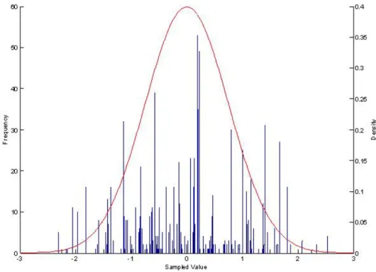
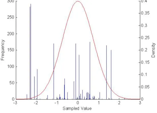
D0 is a specified base distribution, such as a standard normal and λ is a positive scalar precision parameter determining how close draws from DP(λD0) will follow D0. A random distribution D follows a Dirichlet process, DP(λD0), if for any partition of a sample space into categories B1,B2, . . . ,Br, then D(B1), D(B2), . . . , D(Br) has a Dirichlet distribution with parameters (λD0(B1), λD0(B2), . . . , λD0(Br)). As λ → ∞, the sample distribution D → D0, and thus the Dirichlet process degenerates to the parametric distribution D0. More intuitive definitions of the Dirichlet Process have been given; we briefly discuss two of them.

The first definition of the Dirichlet process is via the stick breaking process. Random draws from a Dirichlet process almost surely generate discrete distributions, as can be seen more easily in the stick-breaking formulation of the Dirichlet process.(Ferguson, 1973; Sethuraman, 1994) In the stick-breaking construction, we define a draw,D, from a Dirichlet process as the infinite weighted sum of degenerate point masses δθj, that

place all their mass on pointθj.

D=

∞

X

j=1

(36)

where

wj = zj

j−1

Y

s=1

(1−zs)

zj ∼ beta(1, λ)

θj ∼ D0

That is, samples θj are drawn from the base distribution D0. A ”stick” that is initially of unit length is repeatedly ”broken” to assign a weight, wj, to each θj. Each

wj is broken from what remains of the stick following the previous j−1 breaks. The sum of the weighted point masses is D. Note that if λ is large, small weights will (in expectation) be given to each θj, so any large deviation from the baseline distribution will receive a small weight and D will tend to closely resemble D0, as can be seen in Figure 2.1. A small λ will allow large deviations from D0 to potentially have a large weight and D may not resemble D0, as can be seen in Figure 2.2. The stick breaking representation of the Dirichlet process nicely represents its discrete nature. A result of this is that the probability of sampling the same θj more than once is non-zero. In fact, the discrete nature of the Dirichlet process allows for clustering of data which we will discuss in more detail below.

The second useful way of describing the Dirichlet process is through the P´olya Urn representation. Many statistical distributions can be derived from urn models.(Johnson and Kotz, 1977) The P´olya urn representation serves not only as a way to describe the Dirichlet process but also as a method of implementing Gibbs sampling algo-rithms.(Blackwell and MacQueen, 1973; Escobar, 1994; Ferguson, 1973) Consider a random variable βi which is distributed as some unknown distribution D, which in turn has a Dirichlet process prior, D∼DP(λD0). Samplingβi proceeds as a follows:

1. β1 is sampled from the base distribution,D0.

2. β2 is set equal to β1 with probability p1. Otherwise it is drawn from D0 with probability 1−p1

3. βj is set equal to βk (k = 1. . . j−1), with probability pk; otherwise it is drawn fromD0 with probability 1−

P_k

i=1pi.

(37)

The conditional distribution of βi given β(i) = (β1, . . . , βi−1, βi+1, . . . , βn) is given by:

[βi|β(i)]∼

¡

1−X

j6=i

pj

¢

D0+

X

j6=i

pjδβj

This representation illustrates an important property of Dirichlet processes: the grouping of observations. A series of n draws from a Dirichlet process will be clustered into k (k≤ n) groups. Note that if all draws of βi have the same value, then βi ∼D0. We take advantage of this clustering property to both reduce the dimensionality of the data as well as to cluster effect estimates into groups of disinfection by-products that have similar effects on risk of spontaneous abortion.

2.5.3 The Dirichlet Process Prior in Practice

(38)

2.5.4 Dirichlet Process Priors for Clustering Regression

Co-efficients

While both semi-Bayes and fully-Bayes models are a distinct improvement over stan-dard epidemiologic analytic techniques, they may be unsuitable in two ways. First, results may be sensitive to the assumed prior distribution of βj and a non-parametric prior would be preferable. Second, when sufficient prior information exists the co-efficients may be grouped into exchangeable categories by incorporating second level coefficients. Unfortunately, in many epidemiologic applications, prior knowledge on how to group the coefficients may be unknown and a procedure that allows them to be grouped into clusters based on similarity of effect sizes would be preferred.

An important property of the Dirichlet process prior is its ability to cluster coeffi-cients into groups. Assumingβj ∼Dand D∼DP P(λD0), implies the following prior distribution on βj:(West et al., 1994)

[βj] ∼

λ

λ+k−1D0+ 1

λ+k−1

X

i6=j

δβi (2.7)

were δβi is a point mass at βi. Thus, βj has a probability of being distributed as the

base distribution,D0, or being clustered with any otherβi, i6=j. Group membership is determined by the precision parameterλ, with higher probability of clustering any two coefficients together increasing asλ decreases. At each iteration of the Gibbs sampler, a coefficient is either clustered in a group with some other coefficient(s) or occupies its own cluster. It is important to note that while coefficients will be clustered together during particular iterations of the Gibbs sampler, they will (generally) not be clustered together at every iteration of the Gibbs sampler. So posterior means of coefficients will be similar if the two are frequently clustered together, but are unlikely to be identical.

2.5.5 Gibbs Algorithm for Dirichlet Process Priors

(39)

y = 1 if z >0 = 0 if z <0 z ∼ N(Xβ, σ2_φ

i) β ∼ D

D ∼ DP(λD0)

λ ∼ G(a, b)

D0 = N(µ, τ2)

τ2 _∼ _IG₍_α

1/2, α2/2)

φi ∼ G(ν/2, ν/2)

Unlike the semi-Bayes and fully-Bayes models which specified a particular distribu-tion forβj, the Dirichlet process prior model allows the distribution ofβj to be random. A precision parameter, λ, determines how closely the random distribution follows the base distributionD0. We have placed a gamma prior distribution onλto allow the data to inform about it. The coefficients can be clustered together into k groups that have unique values: γ1. . . γk. For instance,β1 and β4 may have a common valueγ3, whileβ2 and β10 have common valueγ1. We use the notation (j) to denote a parameter’s value when the jth _{element is excluded. For instance,} _β(j) _{= (}_β

1, . . . , βj−1, βj+1, . . . βp). In order to implement a Gibbs sampling algorithm, we need full conditional distributions, however they are not as easily obtained for the Dirichlet process prior model. The necessary full conditionals can be shown to be:

f(z|y = 0,β) ∝ N(Xβ,W) truncated above at 0 (2.8)

f(z|y = 1,β) ∝ N(Xβ,W) truncated below at 0 (2.9)

f(βj|z,y, φ) ∝ pnew,jN

¡

E_jdpp, V_jdpp) + k(j)

X

l=1

pl,jδ_γ(j)

l (2.10)

f(τ|y,β,φ,z) ∝ IG µ

α1+n

2 ,

α2+

P

(γj−µ)2 2

¶

(2.11)

f(φi) ∝ G

µ

ν+ 1

2 ,

ν+σ−2₍_z

i −x0iβ)2 2

¶

(40)

where

E_jdpp = (τ−2₊ n

X

i

x2

ij/φ2i)−1(µ/τ2+ n

X

i

xijh(j)i /φ2i) (2.13)

V_jdpp = (τ−2₊ n

X

i

x2

ij/φ2i)−1 (2.14)

We defineh(j)_i =zi−x(j)

0

i β(j). The full conditional posterior distribution of βj contains the weights:

pnew,j =

λ

λ+p−k(j)₋₁ ×

N(0|µ, τ2₎Q_N₍_h(j) i |0, φ2i)

N(0|E_jdpp, V_jdpp) (2.15)

pl,j =

p

λ+p−k(j)₋₁ × n

Y

i=1

N(h(j)_i |xijβ_l(j), φ2i) (2.16)

The Gibbs sampling algorithm proceeds by first imputing the latent continuous variable z. Second, coefficients β1. . . βp are assigned to clusters γ1. . . γk. Cluster allocation is determined by the weights in equation 2.15 and equation 2.16. For each coefficient, we sample from the multinomial distribution defined by equations 2.15 and 2.16. With probability pnew,j the jth coefficient is assigned to a new cluster or it is assigned to existing cluster l with probability pl,j. After determining the cluster allocation of each coefficient, the third step is to define a new design matrix to reflect the allocation. For example, if we had 4 coefficients that were clustered into groups as follows:

γ1 = β1 =β2 =β4

γ2 = β3

We would then generate a new matrix, R = (r1,r2) where r1 = (x1 +x2 + x4) and r2 = x3. Now, the cluster-specific coefficients can be updated by sampling from

N(Eγ, Vγ), where Vγ = (Σγ−1 +R0W−γ1R)−1 and Eγ =Vγ(Σγ−1µ+RW−γ1z) and Wγ is a matrix with diagonal termsσ2_φ

i.

(41)

2.5.6 Dirichlet Process Prior with Selection Component

Although we wish to estimate the effect of each exposure, we anticipate that in many studies some of the exposures will have no effect. If a given exposure has no effect on the outcome it cannot confound the effect of any other exposure and we would prefer to exclude it from the model. Variable selection techniques in the epidemiologic liter-ature are limited, generally relying on backward or forward selection strategies. These strategies generally look at a large number of models to determine whether individual terms should be included or excluded. A common exclusion criterion in epidemiologic variable selection is that the OR of interest change by less than 10% when the variable is excluded (and frequently includes a component examining whether the variable is an ef-fect modifier as well). A final model is arrived at and is treated as the only model that was examined, a strategy leads to inappropriately small reported variances.(Draper, 1995; Leamer, 1978; Raftery, 1996) However, there has been an increasing focus on variable selection methods in the statistical literature, largely motivated by gene ex-pression applications.(Efron and Tibshirani, 2002; Newton et al., 2001) For example, Geweke proposed a mixture prior, that allows an unknown subset of the predictors to have zero coefficients (βj = 0), while using a normal prior for the remaining coef-ficients.(Geweke, 1996) When using a Dirichlet process prior for the coefficients, the exposures are automatically clustered into groups. By using Geweke’s mixture prior for the group specific coefficients, we allow a cluster of exposures that has coefficients equal to zero. We adopt this prior distribution in the Dirichlet process prior to per-form simultaneous variable selection and clustering which is known to have excellent properties.(Ishwaran and Rao, 2005)

2.5.7 Gibbs Algorithm for Dirichlet Process Prior with

Selec-tion Component

(42)

y = 1 if z>0 = 0 if z<0 z ∼ N(Xβ, σ2_φ

i) β ∼ D

D ∼ DP(λD0)

λ ∼ G(a, b)

D0 = πδ0+ (1−π)N(µ, τ2)

τ2 _∼ _IG₍_α

1/2, α2/2)

φi ∼ G(ν/2, ν/2)

π ∼ beta(a, b)

whereδ0 is a degenerate distribution with all its mass at zero. The probability, π, that a randomly selected coefficient will be zero is given a beta prior to allow the data to help inform about its value.

The Gibbs sampler proceeds as above except the weights for assigning cluster allo-cation are now defined:

pnew,j =

λ(1−π)

λ+p−k(j)₋₁ ×

N(0|µ, τ2₎Q_N₍_h(j) i |0, φ2i)

N(0|E_jdpp, V_jdpp) (2.17)

p0,j = π (2.18)

pl,j =

p(1−π)

λ+p−k(j)₋₁ × n

Y

i=1

N(h(j)_i |xijβl(j), φ2i) (2.19)

These weights are used as parameters in the multinomial distribution as before, with the difference being that now a draw can take the value of another coefficient (pl,j), a new value (pnew,j), or be assigned a value of zero (p0,j). The next step is to update the cluster specific coefficients as before. The only additional step is to update the probability of assigning a coefficient a zero value,π. Its conditional posterior distribution is a function of the number of coefficients assigned a zero value in the last iteration,n0:

f(π|y,β) = beta(a+n0, b+p−n0)

(43)

2.6 Model Specification for Analysis of Disinfection

By-Products and Spontaneous Abortion

We specified a discrete time hazard model for the probability that a spontaneous abor-tion occurs in a given gestaabor-tional week with terms for gestaabor-tional week specific intercepts confounders and 13 constituent disinfection by-products. The concentrations of these by-products were categorized to allow for a more flexible relationship between the logit of the probability of spontaneous abortion and dose, we categorized constituent disin-fection by-products into quartiles, when possible. We implemented the four Bayesian hierarchical models we previously discussed: semi-Bayes, fully-Bayes, Dirichlet process prior, and Dirichlet process with a selection component. We use the existing literature to specify prior distributions for these models. Because the results of any analysis de-pend heavily on modeling assumptions, we performed sensitivity analyses to assess how changes to our prior specifications alter our assumptions.

(44)

(45)

(46)

CHAPTER 3 BAYESIAN METHODS FOR

HIGHLY CORRELATED

EXPOSURE DATA

3.1 Abstract

(47)

3.2 Introduction

3.2.1 Motivation and Background

Highly correlated exposures are ubiquitous in epidemiologic research, and may arise due to an association between the measured exposures and one or more latent factors. For example, pesticide exposures for farm workers tend to be highly correlated because individuals apply multiple pesticides in a year, with choice of pesticide influenced by type of crop.(Alavanja et al., 1996; Kirrane et al., 2005) Another example is the cor-relation in nutrient intake that arises from an individual’s food preferences. Lifestyle factors can also contribute to dependency between exposures, such as smoking, alcohol intake, and illicit drug use.

We depict this correlated exposure problem in more general fashion using the di-rected acyclic graph (DAG) in Figure 3.1. Letx1, . . . , xk denote the levels ofk different exposure variables, let U denote an unmeasured variable or variables explaining the correlation in x1, . . . , xk, and let Y denote the outcome. Researchers will generally be interested in estimating effect measures, β1, . . . , βk, for exposuresx1, . . . , xk. Hence, a common strategy is to fit the logistic regression model:

logit{Pr(Yi = 1|xi1, . . . , xik)} = α0+β1xi1+· · ·+βkxik. (3.1)

Unfortunately, maximum likelihood estimation of the model in equation 3.1 can fail to converge when predictors are highly correlated, and estimated coefficients may be unreliable even when convergence is achieved.

This problem has led many epidemiologists to fit logistic regression models incorpo-rating one exposure variable at a time. However, the other exposure variables may be confounders and, if so, must be included in order to assess the causal effect of any spe-cific exposure.(Greenland et al., 1999) Another commonly-used strategy is to collapse the specific exposure information into summaries, such as a sum across chemicals in a class. Unfortunately, this results in a loss of information, does not allow inferences on effects of specific exposures, and can be sensitive to the summary chosen.

3.2.2 Hierarchical Regression

(48)

vari-able, dependent on parameters. For example in equation 3.1, Yi is a random variable that depends on the parameters α0 and β1. . . βk. Hierarchical regression extends ordi-nary regression models by also treating parameters as random variables that depend on further coefficients through a prior distribution. Estimates obtained through hi-erarchical regression are shrinkage estimators in the sense that they are moved away from the unbiased maximum likelihood estimate (MLE) and toward the center of the prior distribution. The amount of shrinkage is controlled by the variance of the prior distribution. A smaller prior variance causes greater shrinkage. By changing the prior distribution, a wide variety of hierarchical regression models can be specified.

Two types of hierarchical regression models have seen wide use in epidemiologic research: empirical Bayes (EB) and semi-Bayes (SB).(De Roos et al., 2001; Engel et al., 2005a,b; Greenland, 1992, 1993, 1994; Greenland and Poole, 1994; Steenland et al., 2000) These methods vary in how they specify prior distributions on coefficients. A typical prior distribution for βj (where j indexes the k coefficients in equation 3.1) is

N(µ, φ2_{), where}_µ_{characterizes the investigator’s prior knowledge about the true value} of the coefficients andφ2_{is the uncertainty regarding that value. SB and EB procedures} differ in how they treat φ2_{. EB models use the current data to estimate} _φ2_{, while SB} methods offer the researcher an opportunity to specify the prior variance based on substantive knowledge.(Casella, 1985; Greenland, 1994) One process of elicitation for

φ2 _{that may be used in SB procedures is for the researcher to specify a range of values} within which 95% of coefficient values are expected to fall under repeated sampling. This range can be used to calculate a value for the variance term, which is then treated as fixed and used in the hierarchical model.

(49)

resulting in estimates that will generally be more robust than SB methods and provide a more realistic summary of the current state of knowledge than EB methods. We note that although we refer to one particular hierarchical model as a fully-Bayes model, all four hierarchical models that we present are equally Bayesian, including the SB model. Our nomenclature was chosen to be in keeping with existing naming conventions.

3.2.3 Extensions

The SB and FB models have potential disadvantages. First, results may be overly sensitive to the assumed parametric form of the prior distribution. Second, in order for SB and FB methods to shrink parameter estimates towards multiple prior means, the coefficients must be specified into classes (e.g., if the coefficients are the effects of differ-ent pesticides, they could be classified as fungicides or herbicides to allow coefficidiffer-ents in those classes to be shrunk toward different means). In many situations, it may be impossible to specify which effects should be grouped in to which classes, or even how many classes there should be. In this situation, a method that allows the data to guide the clustering of coefficients into classes would be preferable. For this reason, we place a Dirichlet process prior (DPP) on the distribution of the coefficients.(Ferguson, 1973, 1974; Gopalan and Berry, 1998) The DPP allows for non-parametric estimation of βj, while simultaneously clustering the βj into groups based on effect size.

(50)

to have excellent properties.(Ishwaran and Rao, 2005)

3.3 Properties of SB and FB Estimators

SB and FB models have been discussed in detail elsewhere.(Greenland, 1992, 1993, 1994, 2000; Lindley and Smith, 1972) Here, we illustrate some of their properties in the simple setting of an ordinary linear regression model in which covariatesxi1. . . xik are regressed on an outcome yi. For ease of presentation, we assume the linear model has a known error term, σ2_{, and that the covariates are orthogonal (i.e., they are not} correlated).

As mentioned above, the SB model incorporates information on βj through a prior distribution. A typical specification for the SB ordinary linear model is:

[yi|βjsb] ∼ N

µ_Xk

j=1

β_jsbxij, σ2

¶

£ βsb

j

¤

∼ N µ

ηj, φ2j

¶

(3.2)

where the prior mean, ηj, incorporates prior evidence regarding the size of the effect for thejth _{coefficient and}_x

ij may be standardized so they are on the same scale. Prior scientific knowledge may indicate that the prior mean is the same for all coefficients, that it varies across the coefficients (i.e, some coefficients have one prior mean and others have a different prior mean) or that each coefficient has its own mean. For example, ifβ1. . . βkare the effect of pesticides on retinal degeneration, one could assume that the prior knowledge of the effect of pesticides is the same for all pesticides (e.g., no effect: ηj = 0), or that the effect varies over different classes of pesticides (such as fungicide, herbicide, insecticide, etc).(Kirrane et al., 2005) In this case, indicator variables for pesticide class,zlj, can be introduced into the prior distribution by allowing

ηj =

P_p

l=1θlsbzlj. The prior variance, φ2j represents the certainty of the prior evidence that βsb

j has an effect of size ηj. The prior variance could be specified from a meta-analysis or could be calculated by choosing a range within which the researcher believes 95% of effect estimates on this topic would lie. Solving the the standard confidence interval formula for the variance term allows the researcher to specify the prior variance. The lack of a prior distribution on θsb

l or φ2j is the distinguishing feature of SB.

umi-unc-1027.pdf

Bayesian Methods for Highly Correlated Exposures:

an Application to Tap Water Disinfection

By-Products and Spontaneous Abortion

ACKNOWLEDGMENTS

CONTENTS

LIST OF FIGURES

LIST OF TABLES

CHAPTER 1

BACKGROUND

1.1

Spontaneous Abortion

1.2

Disinfection Process

1.3

Disinfection By-products

1.4

Animal Studies

1.5

Previous Research on Disinfection By-products

and Spontaneous Abortion

1.6

Highly Correlated Data in Epidemiology

1.7

Common Methods for Correlated Data

1.8

Hierarchical Models

1.9

Summary

CHAPTER 2

METHODS

2.1

Overview of Right From the Start

2.1.1

Data Collection

2.1.2

Water Sampling

2.2

Overview of Analysis

2.3

Bayesian Analysis

2.4

Markov Chain Monte Carlo Algorithms

2.4.1

Data Augmentation Approach

2.4.2

Gibbs Algorithm for Semi-Bayes

2.4.3

Gibbs Algorithm for Fully-Bayes

2.5

Dirichlet Process Prior

2.5.1

The Dirichlet Distribution

2.5.2

The Dirichlet Process

2.5.3

The Dirichlet Process Prior in Practice

2.5.4

Dirichlet Process Priors for Clustering Regression

Co-efficients

2.5.5

Gibbs Algorithm for Dirichlet Process Priors

2.5.6

Dirichlet Process Prior with Selection Component

2.5.7

Gibbs Algorithm for Dirichlet Process Prior with

Selec-tion Component

2.6

Model Specification for Analysis of Disinfection

By-Products and Spontaneous Abortion

CHAPTER 3

BAYESIAN METHODS FOR

HIGHLY CORRELATED

EXPOSURE DATA

3.1

Abstract

3.2

Introduction

3.2.1

Motivation and Background