Kessler_unc_0153D_14030.pdf

(1)

BAYESIAN NONPARAMETRIC METHODS FOR

HIGH-DIMENSIONAL DATA

David C. Kessler

A dissertation submitted to the faculty of the University of North Carolina at Chapel Hill in partial fulfillment of the requirements for the degree of Doctor of Philosophy in the Department of Biostatistics.

Chapel Hill 2013

Approved by:

Dr. David B. Dunson Dr. Amy H. Herring Dr. Stephanie M. Engel Dr. Hongtu Zhu

(2)

(3)

Abstract

DAVID C. KESSLER: Bayesian Nonparametric Methods for High-Dimensional Data

(Under the direction of Dr. David B. Dunson and Dr. Amy H. Herring)

Bayesian nonparametric (BNP or NP Bayes) methods have enjoyed great strides forward

in recent years. BNP methods embody the belief that inference is best driven by the data

itself with minimal assumptions about the underlying model; this approach has motivated a

wide variety of BNP techniques that have met with with much success.

In the first dissertation paper, we address a long-standing complaint about the nonparametric

priors used in BNP analyses, that they do not necessarily reflect the analyst’s prior belief or

intention, and so are not really Bayesian. In fact, it can be demonstrated that a supposedly

uninformative nonparametric prior framework is actually very informative about certain

aspects of the distribution it models. We develop a novel method to incorporate prior

information about functionals of the unknown distribution, replacing undesirable induced

priors on those functionals with prior distributions that reflect real prior belief. We show

that the new prior enjoys the support characteristics of the original prior, and we demonstrate

with examples the effect of the marginal prior on the quality of inference.

In the second and third dissertation papers, we address challenges in the analysis of

high-dimensional data, with a focus on density regression. Many areas of inquiry, particularly in

genetics research, are concerned with the modeling of a continuous physical trait as some

(4)

for this problem in the context of uncorrelated observations, and apply the technique to a

problem in molecular epidemiology. In the third dissertation paper we expand the method

to address correlated observations. We illustrate the utility of the proposed method in an

application to a family-based data from a whole-genome linkage analysis of a neurological

(5)

To my mother, Ann Munro Kennedy. I wish you could be here to see this.

To my daughter Ella, who put up with a lot of fatherly absences and now thinks that

“data work” is the thing to do. Little Bear, you deserve a lot of credit for helping me learn

patience and perseverance.

Most of all, to my lovely wife Kate, without whose support and encouragement I would

(6)

Acknowledgments

Many thanks go to my advisor, Dr. David Dunson, whose training as an endurance

athlete must have been a valuable asset during these years. He has worked with me through

many difficult parts of this odyssey and I have gotten great benefit from his creativity, his

continued support, and most of all his faith that I could finish.

Thanks to my committee: Dr. Stephanie Engel, Dr. Amy Herring, Dr. Hongtu Zhu, and

Dr. Fei Zou. I have greatly appreciated their participation in this process, their helpful

suggestions, and their availability to discuss details of their work.

Hearty thanks to the good friends I made at UNC, particularly my brothers-in-arms,

Ryan May and Vonn Walter, and my original academic advisor, Dr. Larry Kupper.

The people in the UNC Department of Biostatistics have always worked hard to make

this easier: my gratitude to Melissa Hobgood, Veronica Stallings, Vera Bennett, Evie McKee,

Debbie Quach, David Hill, and Scott Zentz.

Much of this work was done with the support of Training Grant T32ES007018 from the

National Institute of Environmental Health Sciences, National Institutes of Health.

SAS has given me employment, flexibility, and encouragement. I would particularly like

to thank Maura Stokes, Randy Tobias, and Bob Rodriguez.

My collaborators, Dr. Peter Hoff of the University of Washington, Dr. Jack Taylor

of NIEHS, and Dr. Allison Ashley-Koch of Duke University were crucial to my progress.

Peter Hoff in particular gave me hope that things would work out. Dr. Eric Lock and

Heidi Cope at Duke University were instrumental in getting me access to data. I would also

like to thank the individuals and families who participated in the studies that produced the

data.

My in-laws, Ed and Gale Unterberg, have been unwavering in their support.

My family: John Kessler, Mary Clare Kessler, and a long list of Unterbergs, Curtises,

Moburgs, Munros, DeZwartes, Cookes, Larimers, and many others encouraged me to take

(7)

List of Tables

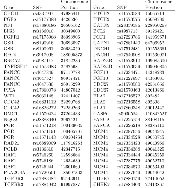
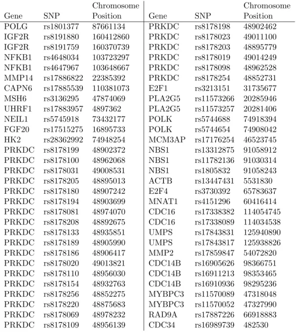
B.1 Details for SNPs included in the final CTF model for

the molecular epidemiology data. . . 94

B.2 Single nucleotide polymorphisms with binary-coded

response profiles matching rs17880594. . . 95

B.3 Single nucleotide polymorphisms with the same

binary-coded response profile as rs9331997. . . 96

binary-coded response profile as rs9331997 (cont’d). . . 97

binary-coded response profile as rs9331997 (cont’d). . . 98

B.6 Comparison of mean square prediction error (MSPE) and coverage proportion (COV) for different methods

applied to molecular epidemiology data. . . 99

C.1 Predictors selected in analysis of full data set, presented

(11)

List of Figures

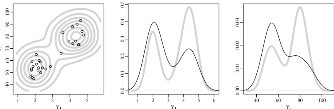
A.1 Population and sample: The left-most panel shows the contours of the population density and a scatterplot of the n = 30 randomly sampled observations. The center and right panels show marginal densities for

the population (light gray) and sample (black). . . 86

A.2 p1priors (black) and kernel density estimates of priors

induced byπI

0 (grey). . . 87

A.3 Comparison of approximatedp0(grey) andp0induced

byπN

0 (black). . . 88

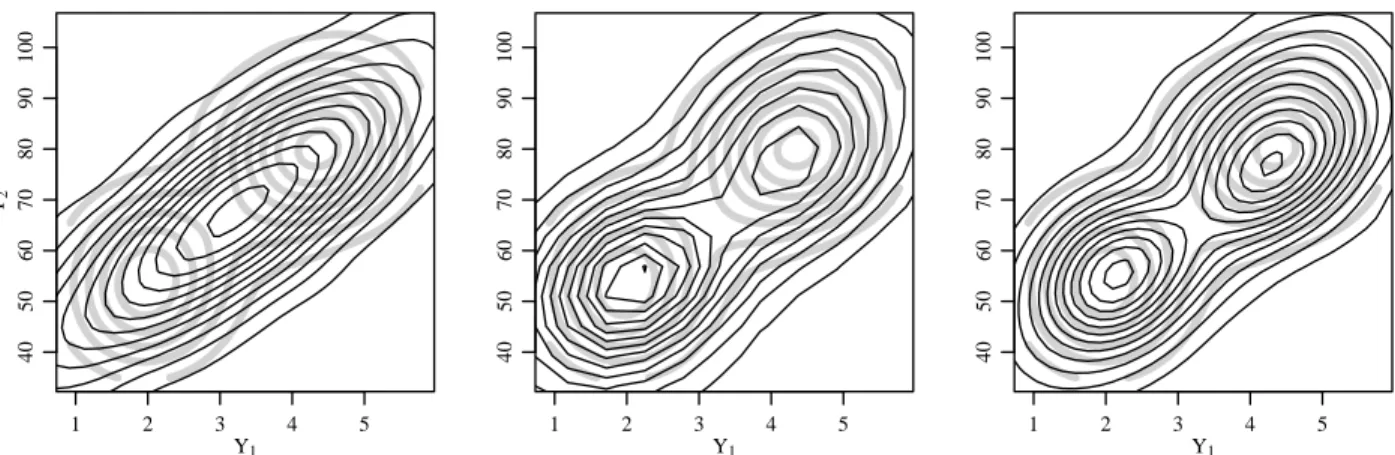
A.4 Contour plots of the posterior predictive density in black and the population density in gray, under πI

0,

πN₀ and π1 from left to right. . . 89

A.5 Marginal population densities and estimates from the three priors: informative DPMM (IDPMM), noninformative

DPMM (NDPMM) and marginally specified prior (MSP). . . 90

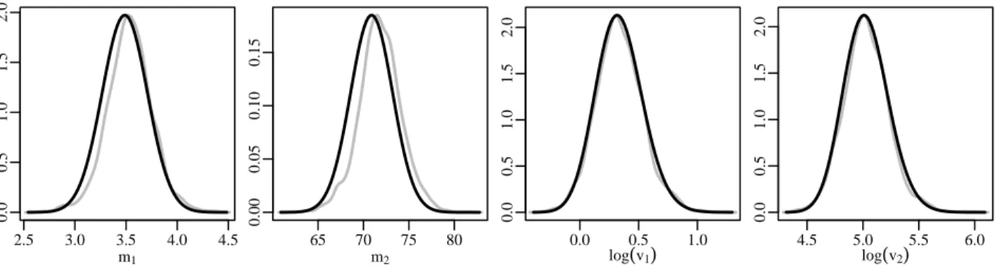
A.6 Priors (gray) and posteriors (black) for the marginal means and log variances. Gray vertical lines indicate the corresponding population values derived from the

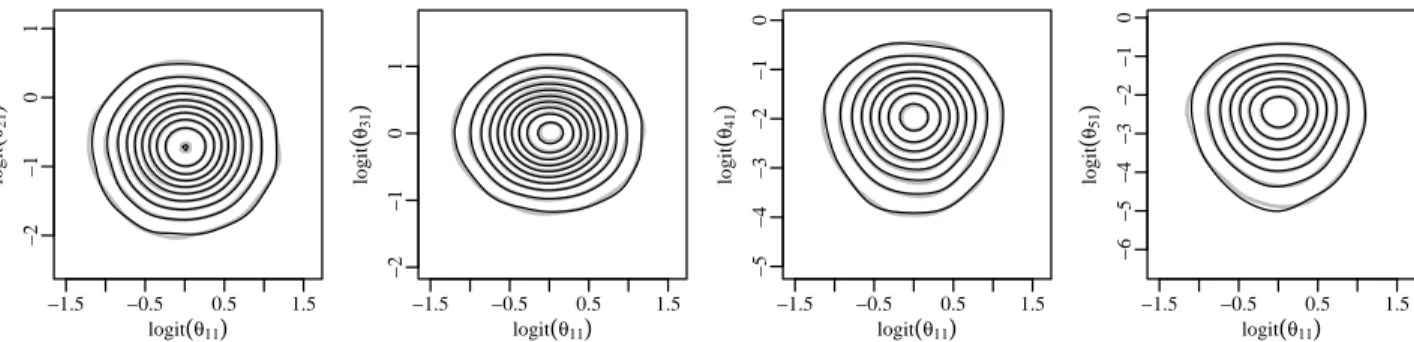
full (n = 272) data set. . . 91 A.7 Comparison of approximatedp0(grey) andp0induced

byπN

0 (black) for a subset of the margins. To facilicate

comparison, a logit transform was used. . . 92

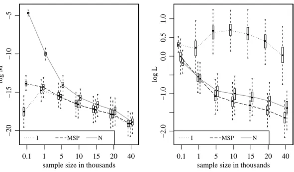
A.8 Comparison of M and L metrics on the log scale for

πI₀ (I), π₀N (N) andπ1 (MSP) at various sample sizes. . . 93

B.1 Conditional densities with similar means but

predictor-dependent higher moments; (Chung and Dunson 2009) . . . 100

B.2 Hypothetical scenario of conditional distributions with

(12)

B.3 Simulation study density; three underlying predictors interact to produce a complex population density. Separate

lines indicate different assumed residual precisions. . . 102

B.4 Simulation study results, demonstrating the improved performance of the CTF in mean square prediction error (MSPE) relative to random forests and comparable performance in coverage (COV) relative to quantile

regression random forests. . . 103

B.5 Selected conditional densities for CTF estimated model of molecular epidemiology data, varying the exposure and the number of copies of the dominant allele at the IGFBP5 SNP. All other SNPs are held at the

“Zero/One Copy” level. . . 104

C.1 Body Mass Index (BMI) data from NHANES 2001-2002. The black curve indicates the empirical BMI density for adults with less than a 9thgrade education; the grey curve is for adults with some college or an associate’s degree. Vertical lines indicate 50th _and 90th percentiles for the separate populations; the 50th

percentile for the two populations is very similar. . . 106

C.2 Summary of simulation study results. Grey dots indicate mean square prediction error (MSPE) for the CTFC method. Black dots indicate mean square prediction

error for the Lasso. . . 107

C.3 First-pass inclusion probabilities for predictors selected in at least one leave-out scenario. Heavy gray vertical lines indicate the range of inclusion probabilities across leave-out sets. Predictors selected in all leave-out scenarios are indicated with darker labels on the horizontal

axis. . . 108

C.4 Conditional densities with varying levels of RS6894946 and age at MRI. Rows indicate different levels of RS6894946 (zero/one copy or two copies of the major allele), and columns indicate different levels of the age at MRI variable. Heavy black lines indicate posterior

(13)

Chapter 1 Introduction

1.1 Literature Review and Motivation

1.1.1 Marginally Specified Priors for Nonparametric Bayes Analysis

In the first paper, we demonstrate a technique for introducing marginal prior information

into nonparametric Bayes (NP Bayes) analyses. Many real-world data analysis situations

are not well-suited to a description that is governed by a finite-dimensional parameter; this

has led to the development of a rich class of NP Bayes methods. These approaches aim to

obtain inference under a prior that has support on the entire space of relevant probability

distributions (Ferguson 1973). These methods have been applied to a variety of problems,

including quantitative trait loci mapping (Zou et al. 2010), density estimation (Muller et al.

1996), regression and classification (Neal 1999), image segmentation (Sudderth and Jordan

2008), speaker diarization (Fox et al. 2011), and functional data analysis (Petrone et al.

2009). This diversity in application reflects the utility of NP Bayes methods in modern

statistical practice.

NP Bayes techniques require some introduction, since the “nonparametric” label is somewhat

(14)

paper, which presented the idea of the Dirichlet process (DP) prior. This paper was titled

“A Bayesian Analysis of Some Nonparametric Problems;” in the NP Bayes setting, the

problem itself is nonparametric, not the analysis. Nonparametric analysis addresses problems

like density estimation and flexible regression models; in both cases the “parameter” to be

estimated has infinite or very high dimension. The attraction of NP Bayes analysis and

nonparametric analysis in general is that structural assumptions about the quantity to be

modeled or estimated are significantly more flexible.

The careful development of NP Bayes techniques has made them successful in the areas

already mentioned. Nevertheless, the complexity of the high- or infinite-dimensional parameter

of interest can make the “Bayes” portion of NP Bayes more challenging. When the parameter

is a complete distribution, a prior on that parameter that is chosen for large support and

convenience in computation can induce priors on functionals of that distribution that are

not consistent with actual information.

We are motivated by situations in which there is reliable prior information about marginal

aspects of an unknown distribution. For example, consider a demographic survey which

collects a small, detailed sample of the population. Assume that an earlier, large-scale census

surveyed a much larger sample of the population, but recorded observations for many fewer

population characteristics. The two surveys, small and large, are not identical and so are

not driven by exactly the same underlying distribution, but they overlap on a few measured

quantities. The Bayesian approach is to use the available prior information from the earlier,

larger survey on those overlapping quantities to inform inference in the newer survey. If

we are using a nonparametric prior for the distribution of interest in the smaller survey, we

may not be able to directly manipulate that nonparametric prior to accommodate this prior

information without inducing undesirable behavior into other aspects of our nonparametric

(15)

we cannot guarantee that this bespoke prior will have the same support as generally applied

nonparametric priors.

Density estimation provides a good example of the utility of NP Bayes approaches and

further illustrates the challenges with the inclusion of prior information. In the nonparametric

Bayes treatment of density estimation, the practicioner need not be restricted by a specific

parametric form such as a multivariate normal. The early work of Ferguson (1973; 1974),

Blackwell and MacQueen (1973) and Antoniak (1974) established theoretical properties for

the Dirichlet process (DP) prior, a prior over probability measures. For a given sample

space Y, a DP prior over distributions on Y is parameterized in terms of a “base measure” Q0 on Y and a “concentration parameter” α. One limiting aspect of the DP prior is

that it produces random measures that are almost surely discrete, making it less suitable

for modeling continuous outcomes directly. To address this, Antoniak (1974), Lo (1984),

and Ferguson (1983) presented the idea of a Dirichlet process mixture model (DPMM),

where the DP prior serves as the prior for a mixing distribution; this provides a more

appropriate method for modeling the distribution of continuous quantities. In that setting,

the data are assumed to come from a population with density p(y|Q) = R p(y|ψ)Q(dψ), where {p(y|ψ) : ψ ∈ Ψ} is a simple parametric family. As Q is discrete with probability 1, the resulting model for the population distribution is a countably infinite mixture model,

where the parameters in the component measures are determined byQ0, and the number of

components with non-negligible weights is increasing in α.

Sampling from the posterior distribution under such a prior is problematic due to its

complexity; MCMC techniques were developed in Escobar (1994) and Escobar and West

(1995). These methods performed well for conjugate DPMs; Kleinman and Ibrahim (1998a;b)

demonstrated the use of DPMs to model the distribution of random effects in the generalized

(16)

In cases where the base measure Q0 is not conjugate to the component likelihood,

the integrations required in the method of Escobar and West can significantly expand

computation time. Ishwaran and James (2001) developed techniques for an alternative

treatment of the DPM, based upon the “stick-breaking” representation for the DP that

was developed by Sethuraman (1994). The Ishwaran and James approach avoids integrating

over the random mixing measure unlike in the Escobar and West method. This makes

non-conjugate base measures in DPM models more feasible than in the P´olya-urn style of

sampler developed in the earlier works. Sampling methods for DPM models evolved with

the introduction of the retrospective sampler (Papaspiliopoulos and Roberts 2008), the slice

sampler (Walker 2007; Kalli et al. 2011) and the exact block Gibbs sampler (Yau et al. 2011).

These continuing improvements in sampling techniques have prompted the application of the

DPM model to an expanding variety of problems.

In the case of the DPMM, the choice ofαandQ0will have a significant effect on the prior

for the population density, and potentially on posterior inference. Many applications include

priors for the base measure (Escobar and West 1995; Muller et al. 1996) and incorporate

estimation of Q0 and α into the posterior inference. Other approaches have addressed the

challenge of specifyingQ0 by applying empirical Bayes techniques to develop a point estimate

for Q0 (McAuliffe et al. 2006). Although it is common to give the base measure an

over-dispersed form in an attempt to avoid an unduly informative prior, such an approach is

actually highly informative in favoring allocation to a single cluster unlessαis appropriately adapted (Bush et al. 2010). The particular case of the DP prior illustrates the general

challenge of incorporating prior information in a nonparametric setting. The results of

Yamato (1984) and Lijoi and Regazzini (2004) can be extended to adjustαandQ0 in normal

DPMMs so that the induced prior expectation and variance of the population mean can be

(17)

Moala and O’Hagan (2010) proposed a method to update a Gaussian process (GP) prior

with expert assessments of the mean and other aspects of an unknown density. As with

the Dirichlet process prior, the GP prior requires specification of the mean and covariance

functions that characterize the GP. These provide a base for the prior in the same way

that the Q0 base measure does for the Dirichlet process prior. In the Moala and O’Hagan

approach, elicitation of these quantities is derived from expert assessments of quantiles of

the unknown distributions.

Many NP Bayes methods for finite sample spaces are built on the Dirichlet distribution

(DD); in this case the unknown parameter π = (π1, . . . , π|Y|−1) can be interpreted as the

parameter of a multinomial distribution. The DD prior is nonparametric in the sense that

it has support on the entire (|Y| −1)-dimensional simplex. Such a prior on a distribution π depends on concentration parameters αj, j = 1, . . . ,|Y|. Large values for these parameters result in a prior concentrated near the center of the simplex, while small values concentrate

the prior at the vertices of the simplex.

This highlights the general challenge with Bayesian methods and the thornier challenge

with nonparametric Bayes methods, the elicitation of a prior. In the usual parametric Bayes

analysis, we are concerned with specifying priors for parameters that have some readily

interpretable effect on the overall model. This can be daunting in complex parametric

models; for example, log-linear models for high-dimensional contingency tables have a large

number of parameters that require prior specifications. In the nonparametric Bayes case, the

parameter of interest has either high or infinite dimension, and elicitation of a meaningful

prior is an even more difficult task.

An increase in dimensionality can quickly become a challenge in the analysis of multivariate

data, whether those data are discrete or continuous. Simply considering the pairwise interactions

(18)

interactions increases as the square of the dimension of the observations. In the case of

categorical data the problem can be even more daunting, particularly if we wish to include

all possible interactions. For example, genetics data is sometimes presented as multivariate

unordered categorical data, with each element in an observation indicating one of four

nucleotides. A sequence of 10 nucleotides then needs 410 ≈ 106 parameters to describe a saturated model, while a sequence of only twice as many nucleotides needs 420 ≈ 1012 parameters. This is clearly intractable for any parametric treatment of this problem that

attempts to address the complete dependency structure.

Frequently, simplifying assumptions are made about the extent of meaningful correlations.

For example, the copula Gaussian graphical model presented in Dobra and Lenkoski (2011)

eliminates some of this complexity through the use of the copula and the accompanying

transformation of categorical variables, but the graphical model introduces additional

simpli-fication of the covariance structure in the transformed space so that elements of the Gaussian

covariance are constrained to be zero. More familiar approaches for multivariate unordered

categorical data, such as the log-linear model in either frequentist or Bayesian analysis, might

also discard higher-order interactions pre-emptively. In the case of maximum likelihood

analysis, a complex model applied to a moderately-sized data set will certainly result in

empty cells in such a high-dimensional multiway contingency table; this will mean that

asymptotic assumptions may not hold (Fienberg and Rinaldo 2007). In Bayesian analysis,

the sheer number of models possible under this scenario may make it extremely difficult for

any one model to appear better than another. Prior specification may also be problematic,

though there exist more sophisticated methods for prior choice in this setting (Massam et al.

2009).

An NP Bayes approach to this scenario was proposed by Dunson and Xing (2009).

(19)

interaction structure to be unknown, and model the joint distribution of all variables as a DP

mixture of product multinomials. In effect, this treats the observations as if they come from

a mixture of subpopulations. Within each subpopulation the variables are conditionally

independent. Marginalizing over the mixing measure for these subpopulations induces

dependence between the several variables, without making strong assumptions about the

nature of that dependence. This substantially reduces the number of parameters within the

model; in the 20 nucleotide example, the number of parameters is linear in the number

of mixture components. This approach results in a sparse structure for the data, but

Bhattacharya and Dunson (2012) pointed out that increasing the dimension of the problem

could result in a proliferation of components, since the entire observation vector is used to

weight the cluster allocations. As an alternative, Bhattacharya and Dunson proposed the

simplex factor model, a more general solution that potentially avoids this difficulty.

These underline the difficulty with prior elicitation in nonparametric approaches. While

it is possible to introduce simplifying assumptions and more nuanced models, the challenge

of making an appropriate prior specification remains. Our goal in the first dissertation

paper is to retain the large support provided by popular nonparametric priors but to allow

the introduction of prior information where such prior information is available, replacing

induced priors with the desired prior.

1.1.2 Density Regression With Many Interacting Predictors

In the second and third dissertation papers, we are motivated by efforts to link quantitative

traits with genetic and other factors. In many cases, the quantitative traits have nontrivial

distributions, even when conditioning on many predictors, and it is unappealing to assume a

smooth parametric form for these conditional densities. Furthermore, such data commonly

(20)

number of observations. Because many phenotypes are associated with more than one locus,

the interaction between multiple loci can be just as important as their separate action. In

these settings of “largep, smalln”, the additional complexity of interactions makes standard methods intractable, and we wish to develop methods that can address predictor selection

at the same time as we consider conditional densities of nontrivial shape. Finally, we wish

to expand these models to accommodate correlated responses, as are found in family-based

studies of complex phenotypes.

A common scenario involves measurements of many single nucleotide polymorphisms

(SNPs) and a continuous, or quantitative, phenotype. In many treatments of this problem,

the strategy is to assess each locus or SNP independently with appropriate controls for overall

false discovery rate (FDR). If it could always be believed that traits of interest are governed

by single factors, then this would be an acceptable approach. However, it seems unlikely

that these traits are so simply explained, and so consideration of multi-factor associations is

desirable.

As discussed in Hoggart et al. (2008), simultaneous consideration of multiple SNPs can

have many advantages. Due to the colossal number of possible multi-factor interactions, this

consideration of many factors simultaneously usually assumes a model where the factors enter

additively, each contributing some part to the quantitative trait. One common approach to

the problem is the Lasso (Tibshirani 1996), which imposes an L1 penalty and limits the

overall sum of coefficients in the additive model, leading to a sparse set of contributing

factors. A corresponding method is ridge regression (Hoerl and Kennard 1970), which uses

anL2penalty, allowing smaller individual contributions to the response from a larger number

of predictors. There are many other methods with the same general approach but using

different penalty structures; for example, the elastic net (Zou and Hastie 2005) combines L1

(21)

While each of these methods has advantages, they all assume strictly additive behavior

for the separate factors, with interactions not considered. Practicioners in genetics are well

aware of the possibility for interaction between SNPs, and there are many methods in the

literature to address the more biologically plausible scenario of multi-factor interaction. Lou

et al. (2007) developed a generalized multi factor dimensionality reduction combinatorial

algorithm. Chen et al. (2007) proposed a forest-based approach to identify gene-gene

inter-actions. Zou et al. (2010) used a Gaussian process prior for the regression function that

incorporated variable selection, enabling selection of a subset of interacting SNPs impacting

the mean of the distribution of a quantitative trait. Yi (2010) surveys statistical approaches

for identifying genetic interactions in high-dimensional settings, including genome-wide

asso-ciation studies (GWAS). Cordell (2009) reviews methods for selecting interactions between

genetic loci contributing to human disease.

None of these approaches directly addresses density regression; we wish to acknowledge

the possibility that the conditional density of quantitative traits given genetic factors may

vary in more than just mean location as a function of those factors. This can be of

considerable interest if the conditional mean does not change appreciably but the variance

or skewness do, so that certain combinations of factors influence the probability of more

extreme forms of the trait.

This assessment of behavior outside of mean shifts has prompted the development of

quantile regression (Koenker and Bassett 1978) methods. These have been used in diverse

areas of genetics research, including the assessment of copy number variation (Eilers and

de Menezes 2005) and the analysis of age-dependent gene expression (Ho et al. 2009).

Quantile regression works with selected quantiles of the response of interest, but we are

more concerned with a characterization of the entire response distribution, and so wish to

(22)

of body mass index (BMI), a measure of health that has certain clinically important cut

points. In particular, individuals with a BMI in excess of 30 are classified as obese and at

higher risk for many debilitating health consequences. A quantile regression approach can

only estimate whether a specific quantile is above or below the point of interest. Density

regression lets us model the entire conditional distribution so that we can identify the quantile

corrresponding to the obesity cutpoint or any other point of interest.

Density regression has enjoyed extensive treatment in the Bayesian literature. The

hierarchical mixture of experts (HME) model (Jordan and Jacobs 1994) gives one of the

most accessible forms of density regression, representing an arbitrary conditional density as

a convex combination of continuous kernels. The expectation maximization (EM) approach

(Dempster et al. 1977) provides an attractive computational framework for estimating the

parameters in these models via maximum a posteriori estimates. Models like the HME

typically assume a specific or maximum number of kernels for the representation. The NP

Bayes literature has developed a number of methods based upon DP mixtures, where the

number of components is one of the parameters to be estimated. DP mixtures have been

adapted in many different ways to the density regression problem, bringing predictors into

the mean functions for the components, the mixing weights, or both.

One approach to conditional density estimation is described in Muller et al. (1996). In

this approach, one estimates of the joint density of the response and the predictors and then

derives a conditional density. This approach has been developed in several other settings

(Shahbaba and Neal 2009; Hannah et al. 2011; Dunson and Xing 2009) and works well in

those applications. One drawback to these joint estimation methods is the need to estimate

the entire joint distribution when we are interested only in a specific conditional distribution.

The additional effort to estimate what becomes a high-dimensional nuisance parameter is

(23)

One challenge to all of these methods is the “curse of dimensionality”, or the increasing

difficulty in obtaining a parsimonious description of the conditional distribution in the

presence of more and more predictors. (Chung and Dunson 2009) proposed methods of

predictor selection in these models, and methods for dimensionality reduction have also

been proposed (Tokdar et al. 2010; Reich et al. 2011), but these encounter difficulty with

larger values of p and do not directly address correlated data.

Random forests (Breiman 2001) provide an approach to density estimation that also

provides support for predictor selection. Nevertheless, the form of the random forest makes

it difficult to assess the role of specific predictors and their influence on the response.

Also, random forests and related ensemble methods do not explicitly address correlated

observations.

This question of correlated data in the presence of many potentially informative predictors

has motived considerable recent research due to the direct relevance for family-based studies

of genetic influences on quantitative traits. Most of this has centered around the adaptation

of the standard linear mixed model (LMM) to high-dimensional predictor sets. Listgarten

et al. (2012) and the related Lippert et al. (2011) propose an LMM-based approach that

uses SNPs to derive a realized relationship matrix between the individuals in the study.

They leverage work by Hayes et al. (2009) demonstrating the advantages of this form of

relationship matrix over that derived from typical pedigree analysis, and develop algorithms

to address the large number of SNPs. In the same direction, Rakitsch et al. (2013) developed

the “LMM-Lasso”, an adaptation of theL1 penalty method to situations involving correlated

observations. These approaches address the important situation of correlated observations

but do not consider the possibility that the conditional density may have a nontrivial form

depending on particular combinations of SNPs.

(24)

density regression in settings with many predictors. In addition to addressing predictor

selection, we wish to produce flexible representations for the conditional density that are

suitable for the investigation of behavior outside of simple mean shifts. We also derive

(25)

Chapter 2 Marginally Specified Priors for

Nonparametric Bayesian Estimation

2.1 Introduction

Many real-world data analysis situations do not lend themselves well to simple statistical

models indexed by a finite-dimensional parameter. This has led to the development of a

rich class of nonparametric Bayesian (NP Bayes) methods, the general idea of which is to

obtain inference under a prior that has support on the entire space of relevant probability

distributions (Ferguson 1973). These methods have been applied to a variety of problems,

such as density estimation (Muller et al. 1996), image segmentation (Sudderth and Jordan

2008), speaker diarization (Fox et al. 2011), regression and classification (Neal 1999), functional

data analysis (Petrone et al. 2009) and quantitative trait loci mapping (Zou et al. 2010) to

name only a few. This breadth of applications reflects the utility of NP Bayes methods in

modern statistical data analysis.

Many NP Bayes methods are built upon either the Dirichlet distribution (DD) for finite

sample spaces or the Dirichlet process (DP) (Ferguson 1973) for infinite sample spaces.

(26)

estimation and inference (Escobar and West 1995) and the steady improvement in sampling

methods (Escobar 1994; Walker 2007; Yau et al. 2011; Kalli et al. 2011) have all made the

DP prior an attractive choice for many applications. For a given sample space Y, a DD or DP prior over distributions on Y is parameterized in terms of a “base measure” Q0 on

Y and a “concentration parameter” α. Although samples from the DP prior are discrete with probability one, this prior is nonparametric in the sense that it has weak support on

the set of all distributions having the same support as Q0. Analogously, the DD prior is

nonparametric in the sense that it has support on the entire (|Y| −1)-dimensional simplex. For both the DD and DP, a large value of α corresponds to a prior concentrated near Q0.

For the DP, a small α results in distributions with probability mass concentrated on only a few points, drawn independently from Q0. For the DD, a small α can result in mass being

concentrated near the vertices of the simplex.

For many NP Bayes methods, the DP is used as a prior for a mixing distribution in a

mixture model: The data are assumed to come from a population with density p(y|Q) =

R

p(y|ψ)Q(dψ), where {p(y|ψ) : ψ ∈ Ψ} is a simple parametric family. A DP prior on Q results in a Dirichlet process mixture model (DPMM) (Lo 1984; Escobar and West 1995;

MacEachern and M¨uller 1998). As Q is discrete with probability 1, the resulting model for the population distribution is a countably infinite mixture model, where the parameters

in the component measures are determined by Q0, and the number of components with

non-negligible weights is increasing in α.

Clearly, the choice ofαandQ0will have a significant effect on the prior for the population

density, and potentially on posterior inference. Many applications include priors for the base

measure (Escobar and West 1995; Muller et al. 1996) and incorporate estimation of Q0 and

(27)

et al. 2006). Although it is common to give the base measure an over-dispersed form in an

attempt to avoid an unduly informative prior, such an approach is actually highly informative

in favoring allocation to a single cluster unlessα is appropriately adapted Bush et al. (2010). In many applications, the base measure is given an overdispersed form in an attempt to

avoid an unduly informative prior. Of course, doing so precludes the incorporation of prior

information into the inference. The particular case of the DP prior illustrates the general

challenge of incorporating prior information in a nonparametric setting. The results of

Yamato (1984) and Lijoi and Regazzini (2004) can be extended to adjustαandQ0 in normal

DPMMs so that the induced prior expectation and variance of the population mean can be

approximately specified (as will be discussed further in Section 3), although specification

beyond the population mean is problematic. Moala and O’Hagan (2010) proposed a method

to update a Gaussian process (GP) prior with expert assessments of the mean and other

aspects of an unknown density. As with the Dirichlet process prior, the GP prior requires

specification of the mean and covariance functions that characterize the GP. These provide

a base for the prior in the same way that the Q0 base measure does for the Dirichlet process

prior. In the Moala and O’Hagan approach, elicitation of these quantities is derived from

expert assessments of quantiles of the unknown distributions.

In this paper, we propose a very general method that allows for the combination of an

arbitrary prior on a finite set of functionals with a nonparametric prior on the remaining

aspects of the high- or infinite-dimensional unknown parameter. In the next section we show

how such a partially informative prior distribution can be constructed from the combination

of any prior distribution on the functionals of interest with the conditional distribution of the

parameter given the functionals under a canonical nonparametric prior. We show that the

resulting marginally specified prior (MSP) inherits desirable features from the canonical

(28)

approximation under the MSP can typically be made via small modifications to any Markov

chain Monte Carlo algorithm applicable under the canonical prior.

In Section 3 we illustrate the use of the marginally specified prior in the context of

multivariate density estimation using normal DPMMs. In an example, we show that existing

approaches to incorporate prior information on mean and covariance into DPMMs lead to

poor density estimates relative to marginally specified priors unless the parametric base

model is an accurate approximation.

In Section 4 we examine the important problem of NP Bayes analysis of large sparse

contingency tables in the presence of prior information on the margins. In this context, we

develop a marginally specified prior from a canonical NP Bayes approach. In an example, we

illustrate how canonical NP Bayes methods designed to be informative on the margins result

in poor performance in terms of margin-free functionals (such as dependence functions). In

contrast, a marginally specified prior accommodates prior information about the population

margins while being minimally informative about other aspects of the population, resulting

in strong performance in terms of both marginal and margin-free aspects of the population.

A discussion of the results and directions for future research follows in Section 5.

2.2 Marginally specified priors: Construction and computation

We consider the general problem of Bayesian inference for a parameter f belonging to a high- or infinite-dimensional space F. For example, Section 3 considers multivariate density estimation over the space of all densities on _Rp _{with respect to Lebesgue measure, and} Section 4 considers the high-dimensional space of multiway contingency tables. In general,

(29)

inference is tractable. Typically, practitioners choose a member π0 of such a class based

on support considerations and the feasibility of posterior approximation, rather than how

well it accurately represents any information we have about specific features of f. In this section, we show how to construct a nonparametric priorπ1 that is informative about specific

features off, but has the same support asπ0 and is “close” toπ0 in terms of Kullback-Leibler

divergence. We also show how MCMC approximation methods for π0 can be modified to

obtain posterior inference under π1.

2.2.1 Construction of a marginally specified prior

Letθ =θ(f) be a function off, such as a population mean ofp(y|f), variance, marginal probability vectors or some finite set of functionals, and let Θ be the range of θ. Any prior distribution π0 on (F,A) induces a prior distributionP0 on (Θ,B) defined by

P0(B) =π0({f :θ(f)∈B}), (2.1)

for each B ∈ B. If π0 is chosen for computational convenience, the induced prior P0 need

not show substantial agreement with available prior information P1 for the functional θ(f).

In some cases a prior π0 selected from a computationally feasible class will make the induced

priorP0 similar toP1: The results of Lijoi and Regazzini (2004) and Yamato (1984) provide

some guidance for Dirichlet process priors if the functionals are means, but in general this will

be difficult. Furthermore, depending on the structure of the nonparametric class, selecting

π0 in order to matchP0 toP1 will result inπ0 being inappropriate for other aspects of f. We

present an example in Section 2.3 to illustrate a case where making π0 highly informative

about θ(f) also makes it highly informative about other aspects of f.

Suppose a nonparametric prior π0 has been identified that is viewed as reasonable in

(30)

does not represent available prior information P1 about θ. The information in P1 can be

accommodated by replacingP0, theθ-margin ofπ0, with the desired marginP1. Specifically, a

marginally specified prior (MSP)π1forf is obtained by combining the conditional distribution

of f given θ with our desired marginal distributionP1 for θ, so that

π1(A) =

Z

Λ0(A|θ)P1(dθ) ∀A∈ A, (2.2)

where Λ0(A|θ) is the conditional probability of A given θ under π0. A prior π1 constructed

this way should have the desired marginal distributionP1 over(Θ,B), and ifP1 P0, should

also have the same support asπ0, since the conditional probabilities under π1 should match

those under π0.

Such a construction is straightforward if f is finite dimensional. Accommodation of nonparametric problems wheref is potentially infinite dimensional requires some additional mathematical detail. We consider the case where A are the Borel sets of a Hausdorff space F, and θ : F → Θ is a measurable map with respect to a σ-algebra B on Θ. Let the prior π0 be a regular probability measure on (F,A), and let P0 be the induced prior distribution

on (Θ,B), i.e., for all B ∈ B, P0(B) =π0({f :θ(f)∈B}).

Example (Dirichlet process mixture model): Recall the Dirichlet process mixture

model prior, defined by

p(y|Q) =

Z

p(y|ψ)Q(dψ)

Q∼DP(α, Q0),

where {p(y|ψ), ψ ∈ _Rp_} _{is a collection of absolutely continuous probability densities over} some Euclidean space Y and Q0 is an absolutely continuous probability measure over Rp.

(31)

mass measures, Q=d P

wkδψk, where ψ ={ψ1, ψ2, . . .} are an infinite i.i.d. sample from Q0,

andwk=vkQ_j<k(1−vj), withv ={v1, v2, . . .}are an infinite i.i.d. sample from a beta(1, α)

distribution. Therefore the prior overQ can be represented as a prior overf = (ψ, v)∈_R∞_. This space, with the usual product topology, is Hausdorff. Now letθ be a moment ofp(y|Q), so that

θ(f) =

Z

g(y)p(y|Q)dy

= ∞

X

k=1

[vk

Y

j<k

(1−vj)]

Z

g(y)p(y|ψk)dy.

The function θ is Borel measurable as long as p(y|ψ) is measurable in ψ for each y ∈ Y. Returning to the marginally specified prior given by (2.2), note that π0(A|θ) is not well

defined on null sets of P0. To make (2.2) meaningful, we restrict attention to informative

prior distributions such thatP1 is dominated byP0. Under this condition and the conditions

on (F,A) and θ given above, the measure π1 on A is well defined and the θ-marginal of π1

is given by P1.

Theorem 1. Let Λ0(·|·) : A ×Θ→ [0,1] be a conditional probability function for π0 given

θ and let P1 be a probability measure on (Θ,B) such that P1 P0. Then π1 : A → [0,1],

defined by

π1(A) =

Z

Λ0(A|θ)P1(dθ),

1. is a probability measure over A;

2. satisfies π1({f :θ ∈B}) =P1(B) for each B ∈ B;

3. is dominated by π0 with Radon-Nikodym derivative

dπ1

dπ0

(f) = dP1 dP0

(32)

For notational economy, we have used θ to represent both an element of Θ and as the function mappingF to Θ, depending on the context. A proof of the Theorem is provided in the appendix.

The MSP π1 constructed above is dominated by π0, but ideally we would like it to have

the same support as π0. Sinceπ1 and π0 share conditional distributions, intuitively it seems

that π1 should have reduced support relative to π0 only if P1 has reduced support relative

toP0. This result can be shown with the aid of the Radon-Nikodym derivative given above,

which implies that π1(A) can be computed as

π1(A) =

Z

A

p1(θ(f))

p0(θ(f))

π0(df) = Eπ0[1(f ∈A)

p1(θ)

p0(θ)],

wherep1 andp0are densities ofP1 andP0 with respect to some common dominating measure

(which could be taken to be P0, for example). Based on this identity, we have the following

result:

Lemma 1. SupposeP1 P0 P1. Then π1 π0 π1.

Proof. It is clear from the definition ofπ1thatπ1 π0. To showπ0 π1, letA∈ Abe a set

such thatπ1(A) = 0. We will show thatP0 P1 impliesπ0(A) = 0. LetBj ={θ :pj(θ)>0}

and Aj ={f :θ(f)∈Bj}so that πj(Aj) = Pj(Bj) = 1 for j ∈ {0,1}. We have

0 =π1(A) = π1(A∩A1)

= Eπ0[1(A∩A1)

p1

p0]

= Eπ0[1(A∩A0∩A1)

p1

p0]. (2.3)

Since p1/p0 >0 on A0 ∩A1, (2.3) implies that π0(A∩A0 ∩A1) = 0. Since π0(A0) = 1, we

(33)

must have 0 =P0(B1c) = π0(Ac1), and so π0(A) = 0.

We also note that π1 has a characterization as the prior distribution that is closest to

π0 in terms of Kullback-Leibler divergence, among priors with θ-marginal density equal to

p1. This follows from re-expressing the probability measures π1 and π0 in terms of densities

with respect to a common dominating product measure, so that

πk(A∩θ−1B) =

Z

B

Z

A

λk(f|θ)pk(θ) µ(df)×ν(dθ)

for k ∈ {0,1}. The Kullback-Leibler divergence is then

D(π1||π0) =Eπ1[ln

λ1(f|θ)p1(θ)

λ0(f|θ)p0(θ)] =Eπ1[ln

λ1(f|θ)

λ0(f|θ)] +Eπ1[ln

p1(θ)

p0(θ)].

Fixing p1, the divergence is is minimized by setting λ1(f|θ) = λ0(f|θ) for θ a.e. P1, i.e.

matching the conditional distributions, giving D(π1||π0) = D(P1||P0).

Lemma 2. Let P1 P0. Then among probability measures π1 on (F,A) with θ-marginal

equal to P1, the Kullback-Leibler divergence of π0 from π1 is minimized when π1(A) =

R

Λ0(A|θ)P1(dθ) for all A∈ A and θ a.e. P1.

A more detailed derivation of this result is given in the appendix.

2.2.2 Posterior approximation under MSPs

(34)

conditional density π(f|y), given by

π(f|y) = p(y|f)π(f) p(y) ≡

p(y|f)π(f)

R

p(y|f0₎_π₍_f0₎_µ₍_df0₎,

whereπ(f) denotes the density ofπ with respect to a dominating measureµ. This represents the conditional measure in that R_Aπ(f|y)µ(df) is a version of the conditional probability π(A|y) for each A∈ A.

For practical reasons the most commonly used priors are those for which there exist

straightforward Gibbs samplers or Metropolis-Hastings algorithms for posterior approximation.

In many cases, simple modifications to these algorithms will allow for the incorporation of

informative priors over functionals of interest. To illustrate, suppose that under priorπ0 we

have a Gibbs sampler for a high dimensional parameter f. Recall that the Gibbs sampler can be viewed as a Metropolis-Hastings algorithm for which the proposals are accepted with

probability one. From this perspective, a Gibbs sampler for approximating the posterior

density π0(f|y) is constructed from proposal distributions with densities J(f∗|f, y) that are

proportional to the posterior density, so that

J(f∗|f, y) J(f|f∗_{, y}₎ =

π0(f∗|y)

π0(f|y)

. (2.4)

For example, decomposing f as {f1, . . . , fK}, the full conditional distribution π0(fk|f−k, y) is one such proposal distribution.

Posterior approximation of π1(f|y) can proceed by using the proposal distributions of

the Gibbs sampler for π0(f|y), but adjusting the acceptance probability. Specifically, the

algorithm for approximating π1(f|y) proceeds by iteratively simulating proposals f∗ from

(35)

probability 1∧rMH, where

rMH =

π1(f∗|y)

π1(f|y)

×J(f|f ∗_{, y}₎ J(f∗_{|f, y}₎ = π1(f

∗_|y₎ π1(f|y)

× π0(f|y) π0(f∗|y)

= p(y|f ∗₎_π

1(f∗)

p(y|f)π1(f)

× p(y|f)π0(f) p(y|f∗₎_π

0(f∗)

= π1(f ∗₎_/π

0(f∗)

π1(f)/π0(f)

.

Let theθ-marginal distribution of π0 be P0, and letπ1 be a marginally specified prior based

on π0 and a θ-marginal distribution P1 P0. Let p0 and p1 be the densities of P0 and P1

with respect to a common dominating measure. By Theorem 1, π1(f)/π0(f) = p1(θ)/p0(θ)

and the acceptance ratio simplifies to

p1(θ∗)/p0(θ∗)

p1(θ)/p0(θ)

.

Similarly, an approximation algorithm for π1(f|y) can be constructed from a

Metropolis-Hastings algorithm for π0(f|y) via the same adjustment. Suppose we have a proposal

distribution J(f∗|f, y) such that the acceptance ratio r0

MH for π0 is computable:

r0_MH = π0(f ∗_|y₎ π0(f|y)

J(f|f∗_{, y}₎ J(f∗_{|f, y}₎

The Metropolis-Hastings algorithm for approximatingπ1(f|y) usingJ(f∗|f, y) has acceptance

ratio

rMH =

π1(f∗|y)

π1(f|y)

J(f|f∗_{, y}₎ J(f∗_{|f, y}₎ = π1(f

∗_|y₎ π1(f|y)

π0(f|y)

π0(f∗|y)

r0_MH = p1(θ

∗₎_/p

0(θ∗)

p1(θ)/p0(θ)

(36)

These results show that an MCMC approximation toπ1(f|y) can be constructed from an

MCMC algorithm forπ0(f|y) as long as the ratiop1(θ)/p0(θ) can be computed. The value of

p1(θ) for each θ ∈Θ is presumably available as p1 is our desired prior distribution for θ. In

contrast, obtaining a formula for p0(θ) will be difficult in some settings. In situations where

the dimension of θ is moderate, one simple solution is to obtain a Monte Carlo estimate of p0 based on samples off fromπ0. Specifically, we can obtain an i.i.d. sample{θi =θ(fi), i=

1, . . . , S}fromf1, . . . , fS ∼i.i.d.π0, and then approximatep0 with a kernel density estimate

or flexible parametric family. The method of approximation will depend on the nature of

θ; the approaches just described are appropriate when p0(θ) is absolutely continuous with

respect to Lebesgue measure. Note that this can be done before the Markov chain is run, so

that the same estimate of p0 is used for each iteration of the algorithm.

In situations where obtaining a reliable estimate of p0 is not feasible, it is still possible

to induce a prior p1 that is approximately equal to a target prior ˜p1, as long as p0 is chosen

to be flat compared to ˜p1. This can be done by replacing p0, the θ-marginal density of π0,

with p1(θ) ∝ p0(θ)˜p1(θ) = Kp0(θ)˜p1(θ). This defines a valid probability density as long as

p0p˜1 is integrable, which is the case, for example, if either density is bounded. In terms of

the MCMC approximation to the resulting marginally specified prior π1, the adjustment to

the acceptance ratio is then

p1(θ∗)/p0(θ∗)

p1(θ)/p0(θ)

= p˜1(θ ∗₎

˜ p1(θ)

,

which is presumably computable as ˜p1is the desired prior density. In this setting, ˜p1 contains

the marginal prior information and p1 takes on a form with computational convenience.

The proposed algorithm is closely related to importance sampling (IS) methods described

in the literature. Besag et al. (1995) detail an IS-based approach for assessing prior sensitivity.

(37)

where h(·) is the original prior used to produce the sample and ˜h(·) is an alternative prior. The similiarity with our proposed method and its use of ratios of the marginally specified

prior p1 to the induced prior p0 is clear; one important distinction is that our method

replaces an induced prior on functionals with an elicited prior on those functionals, rather

than substituting a prior in the main specification.

2.3 Density estimation with marginally adjusted DPMM

Perhaps the most commonly used NP Bayes procedure is the Dirichlet process mixture

model, or DPMM (Lo 1984; Escobar and West 1995; MacEachern and M¨uller 1998). The

DPMM consists of a mixture model along with a Dirichlet process prior for the mixing

distribution. The population density to be estimated and the prior can be expressed as

p(y|Q) =

Z

p(y|ψ)Q(dψ)

Q ∼ DP(αQ0),

whereαand Q0 are hyperparameters of the Dirichlet process prior, withQ0 typically chosen

to be conjugate to the parametric family of mixture component densities, {p(y|ψ) : ψ ∈ Ψ}, to facilitate posterior calculations. In this section we show how to obtain posterior approximations under a marginally specified prior π1 based on a DPMM. The approach

is illustrated with the specific case of multivariate density estimation, for which we take

the parametric family to be the class of multivariate normal densities. In an example

analysis of the well-known bivariate dataset on eruption times of the Old Faithful geyser, we

construct a prior distributionπ1 based on the multivariate normal DPMM with a marginally

specified informative prior on the marginal means and variances. Here, we use a parametric

(38)

underπ1is compared to inference under two standard DPMMs, one where the hyperparameters

are chosen to be informative aboutθand another where the hyperparameters are noninformative.

2.3.1 Posterior approximation

Given a sampley1, . . . , yn∼i.i.d.p(y|Q), posterior approximation for conjugate DPMMs is often made with a Gibbs sampler that iteratively simulates values of a function that

associates data indices to the atoms of Q. In a DPMM, sinceQ is discrete with probability one, a given mixture component (atom ofQ) may be associated with multiple observations. Let g : {1, . . . , n} → {1, . . . , n} be the unknown mixture component membership function, so that gi =gj means that yi and yj came from the same mixture component. Note that g can always be expressed as a function that maps{1, . . . , n} onto{1, . . . , K}, whereK ≤n. Inference for conjugate DPMMs often proceeds by iteratively sampling each gi from its full conditional distribution p(gi|y1, . . . , yn, g−i) (Bush and MacEachern 1996). Additional features of Q and p(y|Q) can be simulated given g1, . . . , gn and the data.

This standard algorithm for DPMMs can be modified to accommodate a marginally

specified prior distribution on a parameter θ = θ(Q). Let f = {g, θ} and let π0 be the

prior density on f induced by the Dirichlet process on Q. Our marginally specified prior is given by π1(f) = π0(f)p1(θ)/p0(θ), where p0 is the density for θ induced by π0 and

p1 is the informative prior density. An MCMC approximation to π1(f|y1, . . . , yn) can be obtained via the procedure outlined in Section 2.2. Given a current state of the Markov

chain f = {θ, gk, g1, . . . , gk−1, gk+1, . . . , gn} = {θ, gk, g−k}, the next state is determined as follows:

1. Generate a proposal f∗ = {θ∗_{, g}∗

k, g−k} from π0(θ, gk|g−k, y) = π0(gk|g−k, y)π0(θ|g, y)

by

(39)

(b) generating θ∗ ∼π0(θ|gk∗, g−k, y).

2. Set the value of the next state of the chain to f∗ with probability 1∧[p1(θ∗)/p0(θ∗)]/[p1(θ)/p0(θ)],

otherwise let the next state equal the current state.

This procedure is iterated over values of k ∈ {1, . . . , n}, possibly in random order, and repeated until the desired number of simulations of f is obtained. Note that steps 1.(a) and 1.(b) compose a standard Gibbs sampler for the DPMM in which posterior inference

for θ is provided, although typically we would only simulateθ once per complete update of g1, . . . , gn. The algorithm for the marginally specified priorπ1 requires that θ be simulated

with each proposed value ofgk so that the acceptance probability in step 2 can be calculated. Implementing the steps of this MCMC algorithm involves two non-trivial computations:

simulation of θ from π0(θ|g, y), and calculation of p0(θ) in order to obtain the acceptance

probability. General methods for the latter were discussed in Section 2.2. For the former, we

suggest using a Monte Carlo approximation to Q based upon a representation of Dirichlet processes due to Pitman (1996). Let K be the number of unique values of g1, . . . , gn and let nk be the number of observations i for which gi = k. If Q0 is conjugate, then the

parameter values ψ(1), . . . , ψ(K) corresponding to the mixture components can generally be

easily simulated. Corollary 20 of Pitman (1996) gives the conditional distribution ofQgiven ψ(1), . . . , ψ(K) and counts n1, . . . , nK as

{Q(H)|ψ(1), . . . , ψ(K), n1, . . . , nK} d =γ

K

X

k=1

1(ψ(k) ∈H)wk+ (1−γ) ˜Q(H),

where γ ∼ Beta(n, α), w ∼ Dirichlet(n1, . . . , nK) and ˜Q ∼ DP(αQ0). A Monte Carlo

(40)

their beta and Dirichlet full conditional distributions. From these values we sample cluster

memberships for a sample of size S from Q using a multinomial(S,{γw1, . . . , γwK,1−γ}) distribution. Note that the countsfor theK+1st category represents the number ofψ-values that must be simulated from ˜Q. To obtain the sample from ˜Q we run a Chinese restaurant process of lengths, and then generate the uniqueψ-values fromQ0 for each partition. This

can generally be done quickly for two reasons: First, the expected number of samples needed

from ˜Q is only Sα/(α+n). For example, with S = 1000, n = 30 and α = 1, we expect to only need about s = 32 simulations from ˜Q. Second, the number of unique values in a sample of size s from ˜Q is only of order logs, which will generally be manageably small.

The marginal sampler we describe above has advantages in terms of efficiency and

convergence rates (MacEachern 1994). However, because it does marginalize out the random

measureQ, we must use the embedded Pitman method to draw samples fromθ(Q) in order to evaluate the Metropolis-Hastings ratio. An alternative approach is to use a stick-breaking

representation that does not integrate out the random measure. We can then use a slice

sampler (Kalli et al. 2011) or exact block Gibbs sampler (Yau et al. 2011) and computeθ(Q) without needing an embedded sampling step, but at the possible expense of lower efficiency

in the sampler.

2.3.2 Example: Old Faithful eruption times

The Old Faithful dataset consists of 272 bivariate observations of eruption times and

waiting times between eruptions, both measured in minutes. To illustrate and evaluate

the MSP methodology we construct two subsets of these data: a random sample of size

n0 = 30 from which we obtain prior information and a second, non-overlapping random

(41)

sampling the observed dataset from the remaining observations. The observed sample had

marginal means (2.97,64.2) and marginal variances (1.29,206.7). The prior sample had marginal means (3.54,71.9) and marginal variances (1.24,134.9). For the purpose of this example, we view the full dataset of 272 observations as the true population. A scatterplot

of the observed data and marginal density estimates are shown in Figure A.1. The observed

dataset consisting ofn = 30 observations clearly captures the bimodality of the population. However, the marginal plots indicate that the sample has overrepresented one of the modes.

Suppose our knowledge of the prior sample is limited to the bivariate marginal sample

meansm0 ∈R2 and sample variancesv0 ∈(R+)2. In such a situation it would be desirable to

construct a prior density p1 over the unknown population marginal means m and variances

v based on the values of m0, v0 and n0, and combine this information with the information

in our fully observed sample to improve our inference about the population. Incorporating

this information with conjugate priors would be straightforward if our sampling model were

bivariate normal, but it is difficult in the context of a DPMM. Proposition 5 of Yamato

(1984) indicates that if the base measure Q0 in the Dirichlet process prior is multivariate

normal(µ0,Σ0), then the induced prior distribution on the mean

R

xQ(dx) is approximately multivariate normal(µ0,Σ0/[α+ 1]). This result is not directly applicable to the multivariate

normal DPMM for two reasons, one being thatQrepresents the mixing distribution and not the population distribution, and the other being that in the conjugate multivariate normal

DPMM the parameter ψ in the mixture component consists not just of a mean µbut also a covariance matrix Σ. Specifically, in the conjugate p-variate normal DPMM, the densityq0

of the base measure Q0 forψ = (µ,Σ) is given by

q0(µ,Σ) = normalp(µ:µ0,Σ/κ0)×inverse-Wishart(Σ :S0−1, ν0) (2.5)

(42)

densities respectively, the latter being parameterized so that E[Σ] =S0/(ν0−p−1). Given

a choice for α it is possible to obtain values of the hyperparameters (µ0, κ0, S0, ν0) so that

the induced prior distributions on the population mean m(Q) = R R yp(y|ψ)Q(dψ)dy and variance V(Q) =R R yyTp(y|ψ)Q(dψ)dy−m(Q)m(Q)T have the following properties:

E[m(Q)] =m0, Var[m(Q)] =

V0

n0−p−1

≈V0/n0 , E[V(Q)] =

n0+α+ 1

n0

n0V0

n0 −p−1

≈V0

(2.6)

Here,m0is the desired prior mean andV0is the desired prior covariance matrix, derived from

the marginal prior information. Within the context of the DPMM, it is difficult to specify the

prior on V(Q) separately from that on m(Q). We construct three different nonparametric prior distributions for a comparative analysis of the Old Faithful data:

• Informative DPMMπI

0: The base measure densityq0 is as in (2.5) with (µ0 =m0, κ0 =

n0/(α+ 1), ν0 =n0, S0 =ν0V0), where the diagonal of V0 isv0, the marginal variances

from the prior sample, and the correlation is equal to the sample correlation from the

observed data. This results in a prior on Qsatisfying (2.6), thereby utilizing the prior information.

• Noninformative DPMM πN

0 : The base measure density q0 is as in (2.5) with (µ0 =

¯

y, κ0 = 1/10, ν0 = p+ 2 = 4, S0 = Sy), where ¯y is the sample mean from the n = 30 values in the observed sample, and Sy is the sample covariance matrix. This prior does not use information from the prior sample, and is designed to promote relative

diffuseness of the induced prior on the marginal population means and variances. Note

that using sample moments for the hyperparameters weakly centers the prior around

the observed data. We can view this as a type of “unit information” prior (Kass and

Wasserman 1995).

(43)

means and marginal variances, we construct a marginally specified prior by replacing

the θ-margin of πN

0 with p1(θ), a product of two univariate normal and two

inverse-gamma densities, chosen to match the prior on θ induced by πI

0 as closely as possible.

Figure A.2 compares p1 with kernel density estimates of the marginal priors induced

byπ₀I. Thus πI

0 and π1 have very similar θ-margins, but otherwise π1 matches the more diffuse

prior πN

0 . We can give π1 any θ-margin we wish, but matching the margins of π0I and

π1 facilitates comparison. The hyperparameter α was set to 1 for all of the above prior

distributions. In order to evaluate the Metropolis-Hastings ratios when approximating the

posterior distribution underπ1, we found that a skewed multivariatet-distribution provided a

very accurate approximation to the joint distribution of the marginal means and log variances

induced by πN₀ . Via a change of variables, this provides an accurate approximation top0(θ),

with which the acceptance probability is computed for approximation ofπ1(f|y). Figure A.3

gives an assessment of the adequacy of this approximation, comparing a smoothed density

estimate of random draws from the approximated p0 with a smoothed density estimate of

random draws from the truep0 induced by πN0.

We ran Markov chains of length 25,000 under each prior, with parameter values being

saved every 10th iteration, resulting in 2500 simulated values of each parameter with which

to make posterior approximations. The chains showed no evidence of non-stationarity and

mixed well under each prior: Based on the dependent MCMC sequences of length 2500, the

equivalent number of independent observations of θ (i.e., the effective sample sizes) were estimated as above 2000 for each element of θ and under each prior. We did sample from the posterior underπ1 using a stick-breaking representation and a slice sampler. The results

were not markedly different from those obtained using the marginal sampler. This slice

(44)

effective sample size of 2500; computational time per independent sample was 95% that of

the marginal sampler.

Posterior predictive distributions under the three priors are shown in Figure A.4. The

informative DPMM provides a poor representation of the population distribution, given in

light gray contours. This is primarily a result of having to set the κ0 hyperparameter to

be moderately large (κ0 = 15) in order to obtain the desired informative prior variance for

the population mean m = (m1, m2). Unfortunately, setting this parameter so high means

that values of µ in the mixture model are tightly concentrated around m0, and so the

multimodality is not captured. In contrast, the posteriors under the noninformative DPMM

πI

0 and the MSP π1 are able to capture the multimodality of the population.

Figure A.5 gives marginal density estimates under the different priors. The figure suggests

that the posterior under π1 is better at representing the underlying population than the

posteriors under the other priors. Recall that the observed sample contains an unrepresentative

number of low-valued observations. The posterior under the non-informative prior πN

0 uses

only the observed data and thus is equally unrepresentative of the population. In contrast,

π1is able to use some information from the prior sample, and is therefore more representative

of the population.

Finally, the marginal posterior distributions of the marginal parameters m and logv are given in Figure A.6. The priors are given in gray and the resulting posterior distributions are

given in black. The population values based upon the full set of 272 observations are given

by gray vertical lines. Across all parameters, π1 gives posteriors that are most concentrated

around the population means. Note that the difference between the priors and the posteriors

underπI

0 is not that large. We conjecture that this is primarily a result of the fact that under

πI

0, most observations are estimated as coming from the same mixture component, thereby