Piercing through Highly Obscured and Compton-thick AGNs in the Chandra Deep Fields. I. X-Ray Spectral and Long-term Variability Analyses

Piercing Through Highly Obscured and Compton-thick AGNs in the Chandra Deep Fields: I. X-ray Spectral and Long-term Variability Analyses

Junyao Li,1, 2 Yongquan Xue,1, 2 Mouyuan Sun,1, 2 Teng Liu,3 Fabio Vito,4, 5 William N. Brandt,6, 7, 8 Thomas M. Hughes,1, 2, 9, 10 Guang Yang,6, 7 Paolo Tozzi,11 Shifu Zhu,6, 7 Xuechen Zheng,1, 2, 12Bin Luo,13, 14, 15

Chien-Ting Chen,16 Cristian Vignali,17, 18 Roberto Gilli,18 and Xinwen Shu19

1_{CAS Key Laboratory for Research in Galaxies and Cosmology, Department of Astronomy, University of Science and Technology of}

China, Hefei 230026, China; [email protected], [email protected]

2_{School of Astronomy and Space Science, University of Science and Technology of China, Hefei 230026, China} 3_{Max-Planck-Institut f¨ur extraterrestrische Physik, Giessenbachstrasse 1, D-85748 Garching bei M¨u nchen, Germany} 4_{Instituto de Astrofisica and Centro de Astroingenieria, Facultad de Fisica, Pontificia Universidad Catolica de Chile, Casilla 306,}

Santiago 22, Chile

5_{Chinese Academy of Sciences South America Center for Astronomy, National Astronomical Observatories, CAS, Beijing 100012, China} 6_{Department of Astronomy & Astrophysics, 525 Davey Lab, The Pennsylvania State University, University Park, PA 16802, USA}

7_{Institute for Gravitation and the Cosmos, The Pennsylvania State University, University Park, PA 16802, USA} 8_{Department of Physics, The Pennsylvania State University, University Park, PA 16802, USA}

9_{CAS South America Center for Astronomy, China-Chile Joint Center for Astronomy, Camino El Observatorio #1515, Las Condes,}

Santiago, Chile

10_{Instituto de F´ısica y Astronom´ıa, Universidad de Valpara´ıso, Avda. Gran Breta˜na 1111, Valpara´ıso, Chile} 11_{Istituto Nazionale di Astrofisica (INAF) – Osservatorio Astrofisico di Firenze, Largo Enrico Fermi 5, I-50125 Firenze Italy}

12_{Leiden Observatory, Leiden University, PQ Box 9513, NL-2300 RA Leiden, the Netherlands} 13_{School of Astronomy and Space Science, Nanjing University, Nanjing 210093, China}

14_{Key Laboratory of Modern Astronomy and Astrophysics (Nanjing University), Ministry of Education, Nanjing, Jiangsu 210093, China} 15_{Collaborative Innovation Center of Modern Astronomy and Space Exploration, Nanjing 210093, China}

16_{Astrophysics Office, NASA Marshall Space Flight Center, ZP12, Huntsville, AL 35812}

17_{Dipartimento di Fisica e Astronomia, Alma Mater Studiorum, Universit`a degli Studi di Bologna, Via Gobetti 93/2, I-40129 Bologna,}

Italy

18_{INAF – Osservatorio di Astrofisica e Scienza dello Spazio di Bologna, Via Gobetti 93/3, I-40129 Bologna, Italy} 19_{Department of Physics, Anhui Normal University, Wuhu, Anhui, 241000, China}

ABSTRACT

We present a detailed X-ray spectral analysis of 1152 AGNs selected in the Chandra Deep Fields (CDFs), in order to identify highly obscured AGNs (NH > 1023 cm−2). By fitting spectra with physical models, 436 (38%) sources with LX > 1042 erg s−1 are confirmed to be highly obscured, including 102 Compton-thick (CT) candidates. We propose a new hardness-ratio measure of the obscuration level which can be used to select highly obscured AGN candidates. The completeness and accuracy of applying this method to our AGNs are 88% and 80%, respectively. The observed logN− logS relation favors cosmic X-ray background models that predict moderate (i.e., between optimistic and pessimistic) CT number counts. 19% (6/31) of our highly obscured AGNs that have optical classifications are labeled as broad-line AGNs, suggesting that, at least for part of the AGN population, the heavy X-ray obscuration is largely a line-of-sight effect, i.e., some high-column-density clouds on various scales (but not necessarily a dust-enshrouded torus) along our sightline may obscure the compact X-ray emitter. After correcting for several observational biases, we obtain the intrinsic NHdistribution and its evolution. The CT-to-highly-obscured fraction is roughly 52% and is consistent with no evident redshift evolution. We also perform long-term (≈ 17 years in the observed frame) variability analyses for 31 sources with the largest number of counts available. Among them, 17 sources show flux variabilities: 31% (5/17) are caused by the change ofNH, 53% (9/17) are caused by the intrinsic luminosity variability, 6% (1/17) are driven by both effects, and 2 are not classified due to large spectral fitting errors.

Li, Xue, Sun et al.

Keywords: galaxies: active — galaxies: nuclei — quasars: general — X-rays: galaxies

1. INTRODUCTION

Highly obscured active galactic nuclei (AGNs), which are defined as AGNs with hydrogen column density (NH) larger than 1023cm−2, are believed to represent a crucial phase of active galaxies. According to our knowledge of co-evolution of supermassive black holes (SMBHs) and their host galaxies (for reviews, see, e.g., Alexander &

Hickox 2012; Kormendy & Ho 2013) and the

hierar-chical galaxy formation model, AGN activity may be triggered in a dust enshrouded environment, into which gas inflows due to either internal (e.g., disk instabili-ties; e.g., Hopkins & Hernquist 2006) or external (e.g., major mergers; e.g., Di Matteo et al. 2005) processes both fuel and obscure the SMBH accretion, resulting in short-lived heavily obscured AGNs (e.g.,Fiore et al.

2012; Morganti 2017). The subsequent AGN feedback

process may blow out the obscuring material and leave out an unobscured optically bright quasar. Compared with unobscured AGNs, AGNs in the highly obscured phase tend to have smaller BH masses, higher Edding-ton ratios (λEdd; e.g., Lanzuisi et al. 2015) and larger merger fractions (e.g.,Kocevski et al. 2015;Ricci et al.

2017a), which may indicate a fast growth state of

cen-tral SMBHs (e.g.,Goulding et al. 2011). Moreover, the cosmic X-ray background (CXB) synthesis models also require a sizable population of highly obscured AGNs, or even Compton-thick (CT) AGNs (NH &1024 cm−2; see, e.g., Comastri 2004; Xue 2017; Hickox &

Alexan-der 2018for reviews), to reproduce the peak of CXB at

20−30 keV (e.g.,Gilli et al. 2007, but seeTreister et al. 2009). Therefore, the study of highly obscured AGNs across cosmic epochs is vital for our understanding of the AGN triggering mechanism, SMBH growth, AGN environment and the origin of CXB.

Thanks to the powerful penetrability of high energy X-ray photons, X-ray observations provide a great win-dow to uncover the mysterious veil of these heavily ob-scured sources that are likely missed in optical surveys. In the past twenty years or so, the deep X-ray sur-veys conducted byChandra (e.g.,Alexander et al. 2003;

Xue et al. 2011, 2016; Luo et al. 2017), XMM-Newton

(e.g., Ranalli et al. 2013),Swift/BAT (e.g., Baumgart-ner et al. 2013) andNuSTAR(e.g.,Lansbury et al. 2017) have provided relatively unbiased AGN samples thanks to their unprecedented depths and sensitivities, which allow us to identify a significant population of heav-ily obscured AGNs (e.g., Risaliti et al. 1999; Bright-man & Ueda 2012;Ricci et al. 2015) using either X-ray color, spectral analysis and/or stacking technique (e.g.,

Alexander et al. 2011; Iwasawa et al. 2012;

Georgan-topoulos et al. 2013;Brightman et al. 2014;Corral et al. 2014;Del Moro et al. 2016;Koss et al. 2016). Moreover, the combination of mid-infrared (MIR), optical and X-ray data provides additional methods to select heavily obscured systems, such as MIR excess (e.g.,Daddi 2007; Alexander et al. 2008; Luo et al. 2011), high 24 µm to optical flux ratio (e.g.,Fiore et al. 2009) and high X-ray to optical flux ratio (e.g.,Fiore et al. 2003).

Among various methods, X-ray spectroscopy pro-vides the most direct and unambiguous way to mea-sure the column density of the obscuring materials. Several previous studies have focused on deriving the intrinsic NH distribution corrected for the survey bi-ases. Tozzi et al. (2006) presented a NH distribution that has an approximately log-normal shape peaking at ∼1023 _cm−2 _{and with an excess at ∼10}24 _cm−2_{. Liu}

et al.(2017) (hereafter L17) reported a similar NH dis-tribution that peaks in a higher NH range, due to the inclusion of more sources with low X-ray luminosities (LX) and high redshifts than that ofTozzi et al.(2006), which are expected to have relatively high NH values. However, both works only focused on bright AGNs, and neither was dedicated to or optimized for investigating highly obscured sources. In particular, L17 excluded CT AGNs in their work and only focused on the Compton-thin population. Hence the absorption distribution and evolution of the most deeply buried AGNs are still un-clear, especially at high redshifts (Vito et al. 2018). Therefore, unveiling the apparently faint, CT regime using the deepest X-ray survey data is indispensable for fully understanding the entire AGN population.

There have also been several attempts to constrain the obscured AGN fraction and CT fraction on the basis of modeling the CXB (e.g.,Gilli et al. 2007;Akylas et al. 2012), the X-ray luminosity function (e.g., Aird et al.

2015; Buchner et al. 2015) or X-ray spectral analysis

highly obscured AGNs are needed to robustly charac-terize the obscuration properties.

Among the X-ray surveys, the Chandra Deep Fields (CDFs) surveys (see, e.g.,Brandt & Alexander 2015and

Xue 2017for reviews), which consist of the 7 Ms

Chan-dra Deep Field-South survey (CDF-S;Luo et al. 2017) and the 2 MsChandra Deep Field-North survey

(CDF-N; Xue et al. 2016) along with the 250 ks Extended

Chandra Deep Field-South survey (E-CDF-S;Xue et al. 2016), provide us the most promising data to study highly obscured AGNs. In particular, the 7 Ms CDF-S, which is the deepest X-ray survey to date, significantly improves the count statistics that allow us to extract high-quality X-ray spectra, detect more faint, highly ob-scured sources and perform more robust spectral analy-ses compared with previous 4 Ms analyanaly-ses (e.g.,

Bright-man et al. 2014). Furthermore, recent works suggest

that the power spectral density (PSD) break frequency of AGN light curves might be related toNH variability (Zhang et al. 2017;Gonz´alez-Mart´ın 2018), which makes obscuration a very important factor in investigating the driving mechanism of AGN variability. Benefiting from the very long timespan of the 7 Ms CDF-S data (16.4 years in the observed frame), we are able to, for the first time, quantify the detailed variability behavior for a large, dedicated sample of highly obscured AGNs, in order to better understand the location of the obscur-ing materials and their contribution to AGN variability (also seeYang et al. 2016, Y16 hereafter).

In this study, we construct the largest dedicated highly obscured AGN sample in the deepest Chandra surveys which enables us to extend the studies of deeply buried sources to lower luminosities and higher redshifts in great details, and present systematic X-ray spectral and long-term variability analyses to study their evolution and physical properties. This paper is organized as fol-lows. We describe our data reduction procedure and sample selection in Section 2. In Sections 3 and 4, we present detailed X-ray spectral analyses of our sample, focusing on the column density and luminosity distribu-tions of highly obscured AGNs as well as their reladistribu-tions; the number counts of CT AGNs and the constraint on CXB models. The reprocessed components, the cover-ing factor of the obscurcover-ing materials and their indica-tions to AGN structures are discussed in Section5. In Section6, by correcting for several observational biases, we constrain the intrinsic NH distribution representa-tive for the highly obscured AGN population and study its evolution across cosmic time. In Section 7, we se-lect a subsample of highly obscured AGNs that have largest counts available and perform detailed long-term X-ray variability analyses, in order to find out the

vari-1.0

1.5

2.0

2.5

3.0

3.5

4.0

log(0.5-7 keV Net Counts)

0

50

100

150

200

N

full sample

highly obscured

variability sample

0

1

2

3

4

5

z

0

100

200

300

N

full sample

spec-

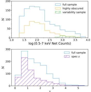
Figure 1. Top: Chandra net counts distributions of the full sample of 1152 AGNs (blue solid histogram), the highly obscured sources confirmed with X-ray spectral fitting in Section4(orange dashed histogram), and the subsample se-lected to perform variability analyses in Section7(solid green histogram), respectively. Bottom: Redshift distributions for the full sample (blue histogram) and the 603 sources with spectroscopic redshifts (purple histogram), respectively.

able fraction as well as the main driven mechanism of variability.

Throughout this paper, we adopt a Galactic column density of NH = 8.8×1019 cm−2 for the CDF-S, and NH = 1.6×1020 cm−2 for the CDF-N, respectively

(Stark et al. 1992). We adopt cosmological parameters

of H0= 70.0 km s−1Mpc−1, ΩM= 0.30, and ΩΛ= 0.70. All given errors are at 1σconfidence level unless other-wise stated.

2. DATA REDUCTION AND SAMPLE SELECTION

de-Li, Xue, Sun et al.

tails). The redshift (spectroscopic redshift) complete-nesses in the CDF-S and the CDF-N main source cata-logs are 99.4% (64.8%) and 95.2% (52.4%), respectively; and the corresponding mean 1σphotometric redshift er-rors are about 0.21 and 0.17, respectively.

The source spectra from individual observations were extracted using the ACIS Extract (AE) software pack-age (Broos et al. 2010). AE generates the point-spread function (PSF) model based on the MARX ray-tracing simulator and constructs a polygonal extraction re-gion that corresponds to an encircled-energy fraction of ∼90%. For crowded sources, AE adopts smaller extraction regions to avoid overlapping polygonal re-gions. The background spectra were extracted using the

BETTER BACKGROUNDS algorithm. The most significant aspect of the above photometry and spectral extrac-tion procedure, compared to the widely used circular-aperture extraction, is that it can obtain photometry and spectra as accurate as possible and remove the con-tamination from neighboring sources to faint sources to the greatest extent (see Section 3.2 ofXue et al. 2011for details). This is extremely important for our work since we are dealing with the highly obscured AGNs that are generally fainter and expected to have limited counts due to significant obscuration.

The spectra eventually used in this work are the merged spectra for which all the individual observations were matched to a commonKs-band astrometric frame

(see Section 2.2.1 inXue et al. 2016) and stacked using the MERGE OBSERVATIONS algorithm in AE. The corsponding response matrix files (rmf) and ancillary re-sponse files (arf) were also generated and combined dur-ing this stage.

We construct our sample by selecting sources which (1) are classified as AGN (TYPE=AGN; see Section 4.5 in Luo et al. 2017 for details); (2) have 0.5–7 keV net counts>20 (FB COUNTS>20) to allow basic X-ray spectral fitting; and (3) have redshift measurements (ZFINAL ! = −1) in the main catalogs. The result-ing full sample consists of 1152 sources, with 660 from the CDF-S and 492 from the CDF-N, respectively. The counts and redshift distributions for the full sample are shown in Figure1. The median counts are 112, and 53% (33%) of the sources have counts larger than 100 (200). The median redshift is 1.45, and 603 (52%) sources have spectroscopic redshifts.

3. X-RAY SPECTRAL ANALYSIS

3.1. Spectral Fitting Models

We use MYTorus-based models (Murphy & Yaqoob 2009) to fit the observed-frame 0.5–7 keV spectra of the full sample in order to identify heavily obscured sources.

Due to limited counts, we do not bin the spectra because it may lose some key information of the sources. We use the Cash statistic (Cstat in XSPEC;Cash 1979) as our spectral fitting statistic. Cstat has a similar probability distribution to χ2 _{statistics and has been proved to be} more appropriate in the low-counts regime. Since Cstat is not appropriate for the background-subtracted spec-tra, we simultaneously fit the source and background spectra, with the latter (with 1642 median counts) be-ing fit with thecplinear model (Broos et al. 2010) that properly describes the observedChandrabackground by a continuous piecewise-linear function in ten energy seg-ments (an example is shown in Figure3). In this way, we are able to maximize the usage of information relevant to the sources.

We adopt two models to fit the source spectra with different components and degrees of freedom (d.o.f) in order to find a statistically robust best-fit one:

1. The MYTorus baseline model: phabs×(MYTZ×

zpow+fref×MYTS +fref×gsmooth(MYTL)).

2. The soft-excess model: phabs×(MYTZ×

zpow+fref×MYTS +fref×gsmooth(MYTL) +fexs× zpow).

These models include all the typical spectral features found in highly obscured AGNs. The phabs compo-nent models the Galactic photoelectric absorption. The MYTZ×zpow term represents the zeroth-order trans-mitted power-law continuum across the torus that takes into account both photoelectric absorption and Comp-ton scattering processes. MYTS andgsmooth(MYTL) stand for the reflection component and the broadened Fe Kα, Kβ fluorescent emission lines, respectively. A second power law is added to represent the soft excess component often found in AGN spectra, possibly origi-nating from the zeroth-order continuum being scattered by the extended Compton-thin (CN) materials in ob-scured AGNs (Guainazzi et al. 2005;Bianchi et al. 2006; Corral et al. 2011). During spectral fitting, the inclina-tion angleθ is fixed at 75◦, which is the average value within a range of 60◦ to 90◦ where the torus intercepts our line of sight (l.o.s). The nominal normalizations of MYTS, MYTL and the second power law are set to be the same as that of the first power law, and we use the constantsfref and fexs to represent the real normaliza-tions. fexs is allowed to vary between 0−0.1, and we assume a 200 keV high-energy cutoff throughout. One thing to mention is that the best-fitNH values in MY-Torus represent the equatorial values, and we always use the l.o.s valuesNH,l.o.s= (1−4 cos2θ)

1

2N_Hin this work.

1

2

5

10

20

50

Energy (keV)

10

10

10

10

10

10

10

ph

ot

on

s c

m

2

s

1

ke

V

1

(a)

pwl

= 2.0, log

= 10

,

= 5%

transimitted

reflection

Fe K + K

soft excess

1

2

5

10

20

50

Energy (keV)

(b)

pwl

= 2.0, log

= 10

,

= 1%

transimitted

reflection

Fe K + K

soft excess

Figure 2. Examples of MYTorus-based models with different parameters used in spectral fitting. The unattenuated continuum (pwl), absorbed continuum (blue curve), transmitted zeroth-order continuum, reflection component, iron emission lines and the soft excess component are shown in different colors. (a) Model used to generate curve A in Figure7withNH, Γ andfexsfixed at 1023cm−2, 2.0 and 5%, respectively. (b) Model used to generate curve B in Figure7withNH, Γ andfexsfixed at 1024 cm−2, 2.0 and 1%, respectively.

1 3 5 7

Energy (keV)

10 5

Co

un

ts

s

1

ke

V

1

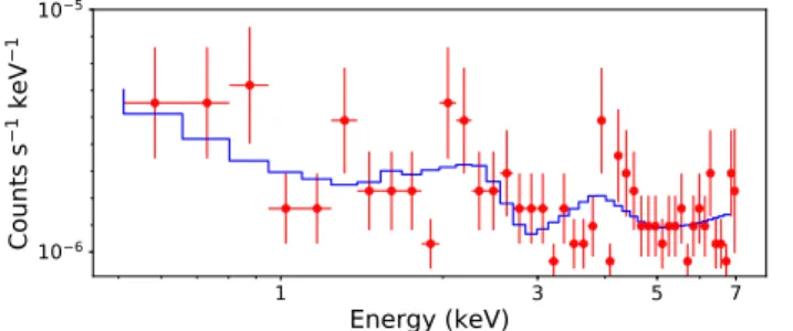
Figure 3. An example of fitting theChandra background spectrum that has 332 counts using the cplinear model (binned only for illustration purpose).

Several previous works suggested that the inclusion of the soft excess and reflection components in the spec-tral models is crucial for us to correctly estimateNHof highly obscured sources (e.g., Brightman et al. 2014;

Lanzuisi et al. 2015). However, the low counts of many

sources do not allow us to apply complex models with free parameters since it could lead to large degenera-cies. Therefore, we choose the model components and the parameter spaces according to the following criteria:

1. We fix Γ at 1.8 (e.g.,Tozzi et al. 2006;Marchesi et al. 2016) for the 851 sources with counts less than 300. For the 301 sources with counts larger than 300, we set Γ free to find a best-fit value.

2. For all sources, we first fit the spectra with a freefref. Iffref is less than 10−5, we then fix it to 10−8that is an arbitrary value set as the lower limit forfref (i.e.,

indicating a negligible reflection component); other-wise, we fixfrefat 1 that is the default value adopted in MYTorus.

3. To determine whether we should add a soft excess component, we compare the Cstat between models with and without considering soft excess emission. The best-fit model is chosen to be the one that has a statistically robust low Cstat value. More specifically, adding a new soft excess component should improve the Cstat at least for ∆C = 3.84 with 1 more d.o.f. This criterion is based on the fact that ∆C approx-imately follows the χ2 _{distribution, thus ∆C = 3.84} is roughly consistent with a > 95% confidence level (Tozzi et al. 2006;Liu et al. 2017).

4. In order to avoid extremely untypical Γ caused by the degeneracy between Γ and NH, we re-fit the spectra of those sources with Γ pegged at 1.4 (i.e., the lowest value permitted by MYTorus) or Γ > 2.4 (i.e., the typical maximum photon index for high-λEdd AGNs; e.g., Wang et al. 2004; Fanali et al. 2013) by fixing their Γ at 1.8. If ∆C=Cfix−Cfree >3.84, we adopt the free Γ value; otherwise, we adopt Γ=1.8.

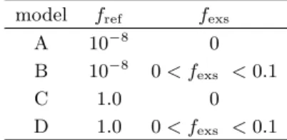
From now on, for convenience, we refer model 1 (2) with negligiblefrefas model A (B) and model 1 (2) with fref fixed at 1.0 as model C (D), as summarized in Table

Li, Xue, Sun et al.

Table 1. Model definitions used in this work

model fref fexs

A 10−8 0

B 10−8 _{0< f}

exs <0.1

C 1.0 0

D 1.0 0< fexs <0.1

validating that the usage of fixed parameters does not significantly affect our results. We also compare our fit-ting results with several previous works (see Section4.1) and those obtained from the Borus model (Balokovi´c et al. 2018; see Section5.3) and find good consistency.

We note that the simple absorbed power-law model (e.g.,phabs×zwabs×zpow; hereafter modelz) has been widely used in the literature to obtain rough estimates of AGN parameters. However, such a model is not ap-propriate for highly obscured AGNs since zwabs only models photoelectric absorption and does not take into account the Compton scattering process, which is par-ticularly important in the high NH regime. Therefore, we also fit the spectra using modelz, aiming at directly testing how accurately such a simple model reproduces the main spectral parameters.

4. SPECTRAL FITTING RESULTS

On the basis of the spectral fitting results, we find that 39% (458/1152) of sources in the full sample are identified to be highly obscured AGNs (hereafter the highly obscured sample; HOS). The main fitting results for HOS using MYTorus models A–D are presented in Table 2 and the full version is available on line. The best-fit models for sources in different count bins and NH ranges are summarized in Table 3. In the follow-ing analyses, we only consider the 436 sources that have the absorption-corrected, rest-frame 2–10 keV luminos-ity (calculated from the lumincommand after deleting all the additional components and only keeping thezpow component)LX>1042erg s−1to avoid possible contam-ination from star-forming galaxies.

4.1. Comparisons With Previous Works and the Model of phabs×zwabs×zpow

Thanks to the increased exposure time, the improved data reduction procedure (see Table 1 inXue et al. 2016 for a summary), the updated redshift measurements and the usage of physically appropriate spectral fitting mod-els for highly obscured AGNs, we are able to extract higher-quality spectra and obtain more robust param-eter constraints than previous works in the same field (e.g.,Tozzi et al. 2006), especially for faint sources. Be-fore performing further analyses, we first make direct

comparisons with several works which presented spec-tral fitting parameters in the CDF-S to understand how different methods influence the spectral fitting results. The works used for comparisons are:

1.Liu et al. (2017) (L17): L17 performed an exten-sive X-ray spectral analysis for the bright sources (hard-band counts >80) in the 7 Ms CDF-S us-ing thewabs×(plcabs×power−law+zgauss+ power−law+plcabs×pexrav×constant) model. The background spectrum was also fitted with the

cplinear model. The redshift information used in the two works is the same.

2.Brightman et al. (2014) (B14): B14 presented

X-ray spectral fitting results in the 4 Ms CDF-S using the BNtorus model (Brightman & Nandra 2011). 112 sources are found common between the two works; 24 of them have redshifts different by more than 0.2 (∆z > 0.2) compared with the values adopted in the updated 7 Ms catalog, and are ne-glected in the following comparison.

3.Buchner et al. (2015) (B15): The 4 Ms CDF-S

spectra were analyzed using a physically motivated torus model and a Bayesian methodology to esti-mate spectral parameters. 114 sources are found common between the two works and 30 of them with ∆z >0.2 are excluded.

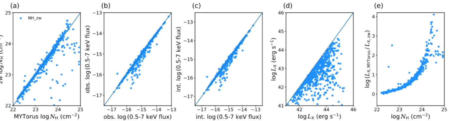
As shown in Figure4, our measuredNHandLXvalues are in general agreement with previous works, despite that for individual sources, the usage of different model configurations and data may result in large discrepan-cies. The largest distinction happens between B14 and our work that ten highly obscured AGNs in our sample are reported to be unobscured in B14. To understand the discrepancy, we re-fit their spectra using the same model and method as described in B14 and the results again confirm their heavily obscured nature. Therefore, the large discrepancy could be due to the adopted data of different depths as well as the different data reduction and spectral extraction methods used in the two works. The comparisons between the results obtained through MYTorus and model z are shown in Figure 5. Note that since MYTorus does not allow NH to vary below 1022 _cm−2_{, a number of unobscured sources are thus} have best-fitNH= 1022 cm−2. Therefore, we only con-sider sources with MYTorus logNH>22.2 cm−2 in the comparison.

Table 2. X-ray spectral fitting results for highly obscured AGNs

XID field RA DEC z ztype HR Γ NH LX counts model

(1) (2) (3) (4) (5) (6) (7) (8) (9) (10) (11) (12)

8 CDF-N 188.841072 62.250256 2.794 zphot 0.17 1.80f 24.42 45.30 39 A 10 CDF-N 188.846392 62.292835 1.173 zphot 0.07 1.80f 23.88 43.15 41 C 11 CDF-N 188.847062 62.217590 1.498 zphot -0.23 1.80f 24.63 44.90 51 D 14 CDF-N 188.853852 62.256847 1.652 zphot 0.59 1.80f 23.81 44.22 105 A 16 CDF-N 188.869802 62.240976 1.732 zphot 0.25 1.80f 23.37 43.97 197 A

Notes. Column 1: source ID in theLuo et al.(2017) andXue et al.(2016) catalogs. Column 2: field. Columns 3 and 4: right ascension (RA) and declination (DEC) for the X-ray source position. Column 5: ZFINAL redshift. Column 6: redshift type

(“zspec”: spectroscopic; “zphot”: photometric). Column 7: hardness ratio. Column 8: photon index (“f”: fixed value). Column 9: line-of-sight column density in units of 1024 cm−2. Column 10: logarithm of absorption-corrected rest-frame 2–10 keV luminosity in units of erg s−1_{. Column 11: 0.5–7 keV background-subtracted net counts. Column 12: best-fit model}

(see Section3.1). The full version of this table is available online.

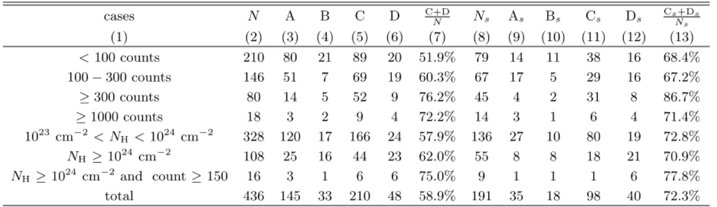
Table 3. The best-fit models for highly obscured sources with 0.5–7 keV net counts<100, 100≤counts<300, counts≥300, counts≥1000, 1023_cm−2 _{< N}

H<1024 cm−2, andNH≥1024 cm−2, respectively

cases N A B C D C+D

N Ns As Bs Cs Ds

Cs+Ds Ns

(1) (2) (3) (4) (5) (6) (7) (8) (9) (10) (11) (12) (13)

<100 counts 210 80 21 89 20 51.9% 79 14 11 38 16 68.4%

100−300 counts 146 51 7 69 19 60.3% 67 17 5 29 16 67.2%

≥300 counts 80 14 5 52 9 76.2% 45 4 2 31 8 86.7%

≥1000 counts 18 3 2 9 4 72.2% 14 3 1 6 4 71.4%

1023 _cm−2 _{< N}

H<1024cm−2 328 120 17 166 24 57.9% 136 27 10 80 19 72.8%

NH≥1024 cm−2 108 25 16 44 23 62.0% 55 8 8 18 21 70.9%

NH ≥1024 cm−2 and count≥150 16 3 1 6 6 75.0% 9 1 1 1 6 77.8%

total 436 145 33 210 48 58.9% 191 35 18 98 40 72.3%

Notes.Column 1: cases of four count bins and twoNH ranges corresponding to CN and CT AGNs. Column 2: total source number in each case. Columns 3−6: numbers of sources that are best-fitted by models A−D, respectively. Note that models C and D havefref fixed at 1.0 while models A and B have negligiblefrefthus negligible reflection component and Fe K lines, and we show the fraction of the sources that have reflection and iron emissions lines in Column 7. Columns 8–13: same as Columns

2–7, but for the spectroscopic-redshift subsample.

dramatically increase withNH. It is obvious that model zunderestimates the intrinsic luminosity due to neglect of the Compton scattering process, and the discrepancy is already evident atNH ∼1023 cm−2 (see alsoBurlon

et al. 2011). Therefore such models with only

photo-electric absorption taken into consideration (e.g.,zwabs, zphabs,ztbabs) must be used with caution in the highly obscured regime.

4.2. Photon Index Distribution

The photon index distribution for the 62 highly ob-scured sources with free-Γ during the fitting process is shown in Figure 6. The mean value of the distribution is 1.82±0.04, in agreement with previous X-ray spectral analyses in the CDF-S (e.g.,Tozzi et al. 2006;Liu et al. 2017) and COSMOS (e.g., Lanzuisi et al. 2013). Note that our Γ distribution peaks at Γ = 1.4 instead of the mean value 1.8. This is because the photon index is

re-stricted within 1.4−2.6 in MYTorus. If we use MYTZ alone which does not limit the Γ range to fit the spectra, most sources with Γ pegged at 1.4 will have smaller Γ, thus the distribution will appear more symmetric with a larger dispersion.

We also try to search the potential correlations among Γ,NHandLXusing the Spearman rank correlation test. No correlation between Γ and redshift (Spearman’sρ= 0.00, p-value = 0.99) is detected, indicating that the inner disk and corona structures have little evolution across cosmic time. The Spearman tests also suggest no significant correlation between Γ andNH(LX).

Li, Xue, Sun et al.

22

23

24

25

26

log

N

H

(This work)

22

23

24

25

26

log

N

H

(L

17

)

41

42

43

44

45

46

log

L

X

(This work)

41

42

43

44

45

46

log

L

X

(L

17

)

22

23

24

25

26

log

N

H

(This work)

22

23

24

25

26

log

N

H

(B

15

)

22

23

24

25

26

log

N

H

(This work)

20

22

24

26

log

N

H

(B

14

)

Figure 4. Comparing the spectral fitting results withLiu et al.(2017),Brightman et al.(2014) andBuchner et al.(2015) for common sources with redshift difference ∆z <0.2.

22 23 24 25

MYTorus logNH(cm2)

22 23 24 25

zw

log

NH

(cm

2)

(a)

NH_zw

17 16 15 14 13

obs. log(0.5-7 keV flux)

17 16 15 14 13

ob

s.

log

(0

.5

-7

ke

V

flu

x)

(b)

17 16 15 14 13

int. log(0.5-7 keV flux)

17 16 15 14 13

int

. lo

g(

0.

5-7

ke

V

flu

x)

(c)

42 44 46

logLX(erg s 1)

41 42 43 44 45 46

log

LX

(e

rg

s

1)

(d)

22 23 24 25

logNH(cm 2)

0 1 2 3 4

log

(

LX,MY

To

ru

s

/

LX,zw

)

(e)

1.2 1.4 1.6 1.8 2.0 2.2 2.4 2.6 2.8

photon index

0

5

10

15

20

N

Figure 6. The distribution of the best-fit photon index for the 62 sources with free Γ. The green and red vertical dashed lines show the median (Γ = 1.77) and mean (Γ = 1.82) values, respectively.

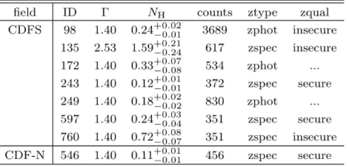
Table 4. Information of sources with extreme photon in-dexes

field ID Γ NH counts ztype zqual

CDFS 98 1.40 0.24+0₋₀._.02₀₁ 3689 zphot insecure 135 2.53 1.59+0₋₀._.21₂₄ 617 zspec insecure 172 1.40 0.33+0₋₀._.07₀₈ 534 zphot ... 243 1.40 0.12+0₋₀._.01₀₁ 372 zspec secure 249 1.40 0.18+0₋₀._.02₀₂ 830 zphot ... 597 1.40 0.24+0₋₀._.03₀₄ 351 zspec secure 760 1.40 0.72+0₋₀._.08₀₇ 351 zspec insecure CDF-N 546 1.40 0.11+0−0..0101 456 zspec secure Notes. Columns are the same as in Table2. The zqual column represents the quality of the spectroscopic redshift (Secure or Inse-cure). For sources with insecure spectroscopic redshifts, the X-ray source catalogs may choose to adopt the photometric redshifts as ZFINAL (see Section 4.4 inXue et al. 2011for details).

indexes are often considered to be reflection-dominated CT candidates and their extremely obscured nature may not be revealed by our best-fit NH (Georgantopoulos

et al. 2009, 2011). Moreover, since we are dealing with the stacked spectra here, sources which possessed large spectral variability may also exhibit untypical spectral shape, as might be the case for XID 249 (see Section 7.4). Additionally, we cannot rule out the possibility that the extreme photon indexes of some sources are wrongly measured due to insecure photometric redshifts.

4.3. Hardness Ratio versus Redshift

For highly obscured AGNs, the significant absorption and scattering of soft X-ray photons may lead to large hardness ratio (HR), thus the HR may be used as an in-dicator of obscuration level (e.g., Wang et al. 2004). In Figure 7 we show the observed HR (here we adopt the definition of HR as (H−S)/(H+S), where H stands for the observed-frame 2–7 keV count rate and S stands for the 0.5–2 keV count rate) as a function of redshift for

0 1 2 3 4 5 6

z

1.00 0.75 0.50 0.25 0.00 0.25 0.50 0.75 1.00

Hardness

curve A : = 2.0, log

N

= 23,

f

= 5%

curve B : = 2.0, log

N

= 24,

f

= 1%

curve C : = 2.0, log

N

= 24,

f

= 5%

Figure 7. Hardness ratio of the highly obscured sample as a function of source redshift. CT candidates selected in Sec-tion4.5with best-fitNH>1024cm−2and the 1σlower limit ofNH>5×1023 cm−2 are shown in red while other highly obscured AGNs are shown in blue. The size of the symbol indicates their best-fitNHvalue. Less obscured sources with best-fitNH <1023cm−2 are shown in gray. Curves in dif-ferent colors represent difdif-ferent selection curves presented in Section4.3.

highly obscured sources and CT candidates confirmed by the spectral fitting as well as less obscured AGNs (best-fit NH < 1023 cm−2) that contaminate our sam-ple. Heavily obscured sources have significantly larger HR than less obscured sources as expected. We also calculate the effective photon index Γeff (obtained by fitting the spectra using XSPEC model phabs×zpow withNH fixed at the Galactic value) for the HOS. 90% of them have Γeff < 1.0, and the median Γeff is only

−0.38 for CT AGNs, which again verify their heavily obscured nature.

Li, Xue, Sun et al.

22 23 24 25

0 20 40 60 80

N

0 1 2 3 4 5

0 10 20 30 40 50 60

42 43 44 45 46

0 10 20 30 40 50

4 3 2 1

0 100 200 300 400

500 Candidate (1%)

Confirmed (1%) Candidate (5%) Confirmed (5%)

23.0 23.5 24.0 24.5

log

N

(cm

)

0.4 0.6 0.8 1.0 1.2

fraction

0 1 2 3 4 5

z

0.4 0.6 0.8 1.0 1.2

42 43 44 45

log

L

erg s

0.4 0.6 0.8 1.0 1.2

4 3 2 1

log

f

0.4 0.6 0.8 1.0 1.2

Completeness (1%) Completeness (5%)

Figure 8. Top: Distributions of source properties of the candidate samples selected from different HR-curves (Candidate) and those confirmed to be heavily obscured through spectral fitting (Confirmed). Bottom: Completeness fractions of the candidate samples selected by different HR-curves. The 1% and 5% in the legend represent different soft excess fractions assumed while deriving the HR-curves in Figure7. Sources without a detected soft-excess component are shown as logfexs=−4 in the plot.

To test whether a simple HR value can be used to select heavily obscured AGNs, we calculate the evolution of HR as a function of redshift for typical X-ray spectral parameters. Since our purpose is to find the critical HR for highly obscured AGNs as a function of redshift, we simply consider the threshold condition: a source with NH = 1023 cm−2. Additionally, we set fref at 1.0, the high-energy cutoff at 200 keV and fix the photon index Γ of the two power-laws at 2.0. The constantfexs is set to 5% that is typical for AGNs with NH ∼1023 cm−2 (e.g.,Brightman et al. 2014). The reason why we adopt Γ = 2.0 instead of the mean value 1.8 is that ∼ 96% of the sources with a well-constrained photon index in L17 have Γ_.2.0. Therefore, with this value we expect that our derived HR curve will be able to successfully select out most of highly obscured AGNs. The model is shown in Figure 2a and the derived model HRs at different reshifts are shown in green in Figure7 (curve A).

It is worth noting that not all CT AGNs have larger HRs than CN AGNs. We also show the HR curve de-rived for a CT AGN with NH = 1024 cm−2. This time fexs is chosen to be 1% due to the fact that fexs de-creases with increasingNH(see Section5.2). The model is shown in Figure2b and the simulated HR curve is also shown in Figure7(curve B). It is clear that at low red-shifts, even a very small soft excess fraction can easily dominate the soft X-ray spectra that could make CT AGNs even softer than CN AGNs. Therefore, to avoid

missing a large number of high-NH sources at low red-shifts, we use curve B atz≤0.8 and curve A atz >0.8 as our selection curve in the following analysis (i.e., the combined curve).

For a source with given HR and redshift values, we consider it as a heavily obscured candidate if the ob-served HR lies above the combined HR curve. By ap-plying this curve to our full sample, 480 sources will be selected as highly obscured candidates (hereafter the candidate sample). 80% (382/480) of sources in the can-didate sample are indeed highly obscured as confirmed from spectral fitting, i.e., the accuracy is 80%. The parameter distributions for the selected candidates and confirmed sources are shown in Figure 8 (top panel). Only 20% of the candidate sources are contaminated by less obscured sources with most of them havingNHonly slightly smaller than 1023 _cm−2 _{and lying close to the} boundary curve, as expected. The redshift, luminos-ity and soft excess fraction distributions for the selected candidates are very similar to sources which are con-firmed to haveNH>1023 cm−2.

most high-redshift and high-luminosity bins. While at lower redshifts and larger fexs, the completeness frac-tion significantly drops to<80%, since the soft excess dominates the observed spectrum which makes highly obscured sources lie below the selection curve.

We also show the result after changing the soft excess fraction for the model CT AGN to 5% (see curve C in Figure 7). This time the completeness fraction at low redshift is improved to 93%, but the accuracy dramati-cally drops to 68% since a large amount of less obscured AGNs are mistakenly included. As a trade-off, we choose to adopt the combined curve A and B as our selection curve. The functional form of this curve can be written as:

HR =

    

   

−0.240z3+ 0.230z2+ 0.680z−0.200, (z ≤ 0.8);

−0.004z3_{+ 0.077z}2_{−0.530z+ 0.740,} (z > 0.8).

(1)

We note that the conclusions in the following sections remain largely unchanged if we use the HR-selected sam-ple instead, suggesting that a simsam-ple HR value can be used to identify highly obscured AGNs and select a rep-resentative highly obscured sample as long as the red-shift and soft excess effects are properly taken into ac-count while deriving the boundary curve.

4.4. Redshift and Luminosity Distributions

In Figure 9 we show the redshift distribution of the HOS in the right-bottom panel. 191 sources have spec-troscopic redshifts and 245 sources have photometric redshifts. The peak appears at z ∼ 1−2.5, which is known as the peak epoch of both star-formation and black hole accretion activities (e.g., Aird et al. 2015). The source amount slightly decreases down to z∼0.5, and significantly drops atz <0.5. SinceChandra only pointed at small patches of sky in these two surveys, the small number of sources detected at z < 0.5 is mainly due to the small volume probed and the insufficient pen-etrability of the corresponding rest-frame energies at low redshifts; thus, the detection probability is severely limited in finding nearby highly obscured AGNs. The downward trend toward high redshifts is primarily due to the flux limits and may be partly due to the fact that photoelectric absorption in the soft band of mildly obscured (NH ∼ 1023 cm−2) sources shifts out of the

Chandra soft bandpass atz∼2.5, making it more diffi-cult to constrainNH (Vito et al. 2018).

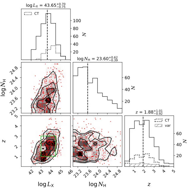
TheLX distribution for the HOS is displayed in the top-left panel of Figure 9. The logLX (LX in units of erg s−1_{) peaks in the range of 43.5–44.0 with the} mean value of 43.65±0.03. The luminous sources with

logLX>44.0 (44.5) account for 32% (11%) of the whole sample. CT AGNs, in particular, have even higher lumi-nosities with the mean value of 44.10±0.06, because of the minimum detectableLXfor a flux-limited survey sig-nificantly increases with increasingNH(see Figure 16). The correlations among LX, NH and redshift are also plotted in Figure 9. The well-known Malmquist bias can be clearly seen in the bottom-left LX-z corner and we will discuss the influence of this bias to our results in Section6.4.

4.5. Observed NH Distribution

The observed distributions of the best-fit NH in six luminosity bins of the HOS are shown in Figure 10. The small amount of high NH sources observed in the smaller LX bins will be clearly illustrated in Section

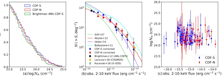
6.2 (see Figure 16) that the minimum detectable lu-minosity significantly increases with NH. We show the normalized cumulative NH distributions in Figure11a. Sources with best-fit NH > 1.0×1024 cm−2 account for ∼25% (108/436) of the HOS. The distribution ob-tained in Brightman et al. (2014), which utilized the 4 Ms CDF-S data, is shown in the same plot for com-parison. The K-S tests imply that theNH distributions from the CDF-S and the CDF-N are consistent withp -value = 0.96, but are different from that inBrightman et al.(2014) withp-value0.001, due to that we iden-tify more sources between logNH = 23.5 – 24.0 cm−2 while the distribution in Brightman et al.(2014) peaks at logNH= 23.0 – 23.5 cm−2.

Li, Xue, Sun et al.

20

40

60

80

100

N

log

LX

= 43.65

+0.70

_0.75

CT

23.2

23.6

24.0

24.4

24.8

log

N

H

20

40

60

N

log

N

H

= 23.60

+0.62

0.39

42 43 44 45 46

log

LX

1

2

3

4

5

z

23.2 23.6 24.0 24.4 24.8

log

NH

1 2 3 4 5

z

20

40

60

N

z

= 1.88

+1.01

_0.92

CT

var

Figure 9. The triangle plot of the correlations amongLX,NHand redshift. The outer parts of the triangle show the distributions ofLX,NH and redshift from the top-left to the bottom-right panels, respectively. The vertical dashed lines show the median value for each distribution. In the redshift andLXdistribution panels, the solid histograms represent the total sample and the dotted ones show the distributions of CT candidates selected in4.5. The shaded histogram shows the redshift distribution of our variability sample in Section7. The inner parts of the triangle show the scatter plots and corresponding density maps overlaid with contours amongLX,NH and redshift, respectively. In theLXversuszplane, the green rectangle shows the subsample we select in Section6.5to investigate the evolution of the intrinsic fraction of CT AGNs among highly obscured ones.

We note that atf2−10 keV>10−15 erg cm−2 s−1, the number of our CT AGNs in the CDF-N (22 sources) is higher than Georgantopoulos et al. (2009) which pre-sented 10 CT candidates in the same field. This may because ofGeorgantopoulos et al.(2009) mainly focused on searching reflection-dominated CT AGNs and possi-bly missed some transmission-dominated sources. We also fit the 22 CT candidates using the BNtorus model (Brightman & Nandra 2011) and find that 20 sources

have best-fit NH > 1024 cm−2 and f2−10 keV > 10−15 erg cm−2 _s−1_{, which confirms the MYTorus result.}

4.6. Number Counts for Compton-thick AGNs

23 24 25

log

N

(cm

)

0 10 20 30 40 50 60

N

logLX< 43

23 24 25

log

N

(cm

)

0 10 20 30 40 50 60

N

43 < logLX< 43.5 43.5 < logLX< 44

23 24 25

log

N

(cm

)

0 10 20 30 40 50 60

N

44 < logLX< 44.5 44.5 < logLX< 45 logLX> 45

Figure 10. The observedNHdistributions in sixLXbins. The small number of highNHsources in lowLXbins is due to that such sources are difficult to detect. This bias will be corrected in Section6.4.

23.0 23.5 24.0 24.5 25.0

(a)log

N

(cm

)

0.0 0.2 0.4 0.6 0.8 1.0

N

CDF-S CDF-N

Brightman 4Ms CDF-S

10 16 ₁₀15 ₁₀14

(b)obs. 2-10 keV flux (erg cm

_s

₎

100

101

102

103

N

(>

S

,d

eg

2

)

Gilli+07 Akylas+12 Ueda+14 Balleytane+11 CDF-S corrected CDF-N corrected Brightman+12 (4Ms CDFS) Lanzuisi+18 (COSMOS) Kocevski+18 (X-UDS)

16.0 15.5 15.0 14.5 14.0

(c)obs. 2-10 keV flux (erg cm

_s

₎

23.0 23.5 24.0 24.5 25.0 25.5 26.0

log

N

(cm

2

)

CDF-S

CDF-N

Figure 11. Left: Normalized cumulativeNHdistribution for our highly obscured sample. The 4Ms CDF-S result adopted from Brightman et al.(2014) is also plotted for comparison. Middle: The observed logN−logS for CT candidates compared with previous number counts in the 4 Ms CDF-S (Brightman & Ueda 2012), X-UDS (Kocevski et al. 2018) and COSMOS (Lanzuisi et al. 2018) as well as several CXB model predictions (Gilli et al. 2007;Ballantyne et al. 2011;Akylas et al. 2012;Ueda et al. 2014). Right: Column density of CT AGNs as a function of observed 2–10 keV flux in the CDF-S (blue) and CDF-N (red), respectively.

we assign a weighting factor 1/ωarea(see Section6.2for details) for each source while calculating their cumula-tive number counts. The corrected results are shown in Figure 11b, and several number counts measurements presented in previous works in the 4 Ms CDF-S ( Bright-man & Ueda 2012), X-UDS (Kocevski et al. 2018) and COSMOS (Lanzuisi et al. 2018) fields are also displayed for comparison. Note that Brightman & Ueda (2012) reported the result in the 0.5–8 keV band and we con-vert the 0.5–8 keV flux into 2–10 keV by assuming a Γ =−0.4 power-law which is the median effective pho-ton index for our CT AGNs.

The corrected number counts for the CDF-S and CDF-N are generally consistent within the error bars

Li, Xue, Sun et al.

We also compare the observed logN−logS with sev-eral CXB model predictions in z = 0−5 (Gilli et al. 2007; Ballantyne et al. 2011; Akylas et al. 2012; Ueda et al. 2014). For the Gilli et al. (2007)1, Akylas et al. (2012)2_{andUeda et al.(2014)}3_{CXB models, the}

lumi-nosity range used to derive the predicted number counts is logLX = 42−45.5 erg s−1, similar to our sample; while for the Ballantyne et al. (2011) model, the pre-dicted result is presented in logLX= 41.5−48 erg s−1. As can be seen from Figure 11b, our observed logN− logS prefers the moderate CT number counts as pre-dicted by Akylas et al. (2012) and Ueda et al. (2014), while other models more or less overestimate or under-estimate the number counts.

In summary, the observed parameter distributions and relationships presented in this section provide a basic description of the highly obscured AGN population and are crucial for distinguishing various CXB models. How-ever, these observed distributions, in particular, the ob-servedNHdistribution, are influenced by several biases. We will discuss more details about these biases and re-construct the intrinsicNHdistribution representative for the highly obscured AGN population in Section6.

5. THE ORIGIN OF HEAVY X-RAY OBSCURATION

5.1. X-ray Highly-Obscured Broad-Line AGNs

We collect optical classification results for our CDF-S sample by cross-matching their optical/NIR/IR/radio counterpart positions presented in the X-ray source cat-alogs (CP RA and CP DEC) with theSilverman et al. (2010) E-CDF-S optical spectroscopic catalog using a 0.500 matching radius. Among the 55 matched sources, 31 sources have been classified. To our surprise, 19% (6/31) of them are labeled as broad-line AGN (BLAGN). The detailed information of these sources are summa-rized in Table5.

Most of the six sources have sufficient counts and re-liable redshift measurements to constrain NH. Three sources have insecure spectroscopic redshifts although they are labeled as BLAGN, and the 7 Ms main cata-log chooses to adopt the photometric redshift as ZFI-NAL for two of them. This could be due to that they have low S/N optical spectra or only one emission line is available for sources within particular redshift ranges, which makes it difficult to conclusively determine the

1 _{http://www.bo.astro.it/}∼_{gilli/count.html/. We assume a} high-zdeclined LF (Vito et al. 2018).

2 _{http://indra.astro.noa.gr/xrb.html. We assume a 40% CT} fraction and the default 4.5% reflection fraction.

3_{http://www.kusastro.kyoto-u.ac.jp/}∼_{yueda/xrb2014.html}

line nature, thus giving an insecure redshift. For three sources with insecure redshifts, we set redshift as a free parameter in the spectral fitting and obtain the best-fit X-ray redshift and corresponding NH. All of them are still best-fitted byNH>1023 cm−2. The redshift range in which the source will remain X-ray highly obscured is also listed. In general, the NH estimates for the six sources are robust. This result suggests that the heavy X-ray absorption in a fraction of sources is largely a l.o.s effect caused by some compact clumpy clouds obscuring the central X-ray emitting region, but the global cov-ering factor (CF) for the high-NH materials is limited thus the BLR is not blocked; or maybe the heavy X-ray obscuration is produced by the BLR itself.

5.2. Soft Excess Fraction Dependences

There are 80 sources in our sample that require a sec-ond power law to fit the soft excess component. The origin of this component is still a puzzle. Many different models, e.g., warm Comptonization or blurred ionized reflection from the disk, partially ionized absorption in a wind, or power-law continuum in other directions scat-tered into the line of sight from large-scale Compton-thin matters, are proposed to explain the diverse situa-tions found in different sources (e.g.,Boissay et al. 2016). However, for highly obscured AGNs, the scattered mech-anism is preferred since either blurred reflection or warm Comptonization from the accretion disk will be signifi-cantly attenuated by the obscuring materials.

We show the fexs, which represents the relative nor-malization of the soft component with respect to the intrinsic power law, as a function of NH in Figure 12. We find a significant anti-correlation between the two parameters: Spearman’sρ=−0.66,p-value =0.001. The mean fexs is 3.7% for the total sample. The scat-tered fraction decreases from 6.1% to 4.3% and 1.3% for NH <5 × 1023 cm−2, 5 ×1023 cm−2 < NH < 1.5× 1024 cm−2 andNH >1.5×1024 cm−2, respectively.

To verify that this anti-correlation is not caused by the parameter degeneracy that sources with a large soft ex-cess fraction and a highNHmight be misclassified as low NH, lowfexsand low intrinsic luminosity sources owing to the low S/N, we assume that CT AGNs have exactly the samefexsas CN AGNs (here we simply choosefexs= 5%). Then we generate fake spectra using model D for a sample of simulated sources, which have redshifts and NH uniformly distributed between z = 0−4 with an interval of ∆z= 0.5 and 23 cm−2_<logN

Table 5. Information of X-ray highly obscured BLAGNs in the CDF-S

XID model fref Oclass z ztype zqual counts logNH(cm−2) z-range zx logNH,x(cm−2)

(1) (2) (3) (4) (5) (6) (7) (8) (9) (10) (11) (12)

882 A 1 BLAGN 3.19 zspec Secure 80 23.1 – – –

944 C 1 BLAGN 0.96 zphot Insecure 69 23.9 all 2.00 24.1

16 A 1 BLAGN 3.10 zphot Insecure 409 23.7 z >1.4 1.66 23.2

399 C 1 BLAGN 1.73 zspec Secure 1077 23.2 – – –

968 C 1 BLAGN 2.03 zspec Secure 500 23.8 – – –

977 C 1 BLAGN 4.64 zspec Insecure 225 23.9 z >1.2 3.25 23.9

Notes. Column 4: optical classification result fromSilverman et al.(2010). 31 X-ray highly obscured AGNs in our CDF-S sample have optical classification results and 6 of them are identified as BLAGNs. Column 10: the redshift range for sources with insecure redshifts to

be determined as being X-ray highly obscured. Column 11: the best-fit X-ray redshift by setting redshift as a free parameter during spectral fitting. Column 12: best-fit logNHwhen adopting the X-ray best-fit redshift. Other columns have the same meaning as Table2.

NH and fexs. The Spearman’s ρ ≈ 0.1 (insensitive to the simulated spectral counts), indicating no apparent correlation, thus the observed anti-correlation is intrin-sic.

By assuming that the second power law originates from the scattered-back continuum,Brightman & Ueda (2012) found that the scattered fraction depends on the opening angle, i.e., sources with small opening angles have lowerfexs. Moreover,Ueda et al.(2015) and

Kawa-muro et al. (2016) found that the [O III] and [O IV] to hard X-ray luminosity ratios are lower in low scatter-ing fraction sources, inferrscatter-ing that the low fexs AGNs are buried in small opening angle torus. Therefore, the anti-correlation betweenfexs andNH indicates that high NH sources might preferentially reside in high CF toruses. This is also consistent with the results from Brightman & Ueda (2012) and Lanzuisi et al. (2015), who found a similar anti-correlation between fexs and NHand explained it as highly obscured AGNs being also heavily geometrically obscured (but see the discussion in the next section).

5.3. Reprocessed Components and Covering Factor

Unlike local CT AGNs in which the prominent neutral Fe lines and reflection hump (hereafter the reprocessed components) are prevalently detected in the high-quality hard X-ray spectra and can be served as unambiguous signatures of being Compton-thick (e.g.,Tanimoto et al. 2018; Zhao et al. 2019; Marchesi et al. 2019), there are 41% of our highly obscured sources and 38% of the CT candidates having negligible fref(see Table 3), respec-tively. It should be noted that the low detection rate of reprocessed components is not in conflict with their highly obscured nature. The poor S/N for low-count sources and the narrowChandra spectral coverage make it challenging to detect narrow iron lines and to distin-guish the transmission and reflection components, which may cause a significant overestimation of the fractions.

0.1

0.5

1

5

10

N

(10

cm

)

0.00

0.02

0.04

0.06

0.08

0.10

0.12

0.14

f

ex

s

Figure 12. The soft excess fractionfexs as a function of

NH. The blue points show the individual sources and the red points show the binned results. The negative correla-tion between fexs and NH indicates that a portion of high

NH sources might have higher “torus” covering factors that makes the soft excess photons hard to escape, under the as-sumption that the excess originates from the scattered-back continuum in highly obscured AGNs.

But we note that it is possible that highly obscured AGNs may have weak reprocessed components if the global CFs of high-NH materials are low or the cen-tral AGN is geometrically fully buried by CT materials such that even the reflected photons cannot escape (e.g., Brightman et al. 2014). To distinguish different scenar-ios, we use the Borus model (Balokovi´c et al. 2018)4_,

which allows CF to vary freely, to fit the spectra for all sources with counts>200. This time we treat pho-ton index as a free parameter in order to make a direct comparison between the two models. The distribution of the derived CFtor, which is defined as the cosine value of the opening angle θtor measured from the symmetry

4_{In the Borus model, CF}

tor= 1.0 corresponds to a fully covered torus while CFtor= 0.1 represents a typical disk-like covering (see

Li, Xue, Sun et al.

0.0 0.2 0.4 0.6 0.8 1.0

CF

0

10

20

30

40

50

N

(a)

fref 1 fref= 1

1.4 1.6 1.8 2.0 2.2 2.4 2.6

photon index (MYTorus)

1.4

1.6

1.8

2.0

2.2

2.4

2.6

photon index (Borus)

23.0

23.5

24.0

24.5

log

N

(MYTorus)

23.0

23.5

24.0

24.5

log

N

(B

or

us

)

42

43

44

45

log

L

(MYTorus)

42.0

42.5

43.0

43.5

44.0

44.5

45.0

45.5

log

L

(B

or

us

)

10

10

10

10

10

10

ke

v

2

(p

ho

to

ns

cm

2

s

ke

V

1

)

ID : 746

(b)

total, CF=0.1 transmission reflection total, CF=1.0 transmission reflection

1 2 CF=0.1

0.5

1

2

3

5

7

Energy (keV)

2 CF=1.0

residual

Figure 13. (a) The covering factor derived through the Borus model (Balokovi´c et al. 2018) and the comparisons between photon index, NH, and LX obtained from the Borus and MYtorus models. The photon indexes in this plot are the original results without fixing Γ at 1.8 for some extreme cases. (b) The spectral fitting result for CDF-S XID 746 using the Borus model. Both the fully buried model (CFtor = 1.0; Cstat = 942.3) and the weak torus model (CFtor = 0.1; Cstat = 941.8) can well reproduce the data. The contribution from the reflection component to the total spectrum in both models are largely negligible.

axis towards the equatorial plane, is shown in Figure 13a. We also show the comparisons of the main spectral fitting parameters with those obtained from the MY-Torus model and find good consistency.

For sources with negligible reprocessed components in the MYTorus model (fref 1), the Borus results are consistent with the weak torus scenario (CFtor ≈0.1), which might suggest that their heavy obscuration is sim-ply a l.o.s effect (i.e., some high-column-density clouds on various scales along our sightline may obscure the compact X-ray emitter), without the necessity to in-voke a strongly-buried nuclear environment. In con-trast, sources with fref = 1.0 are mostly best fitted by a highly-covered model (0.8 < CFtor < 1.0) that have torus covering angles (90◦ −θtor) between 65◦ −90◦. We emphasize that though the l.o.s and the global torus NH are linked in the spectral fitting, those fully-buried sources do not need to be covered by very highNH ma-terials in all directions, since the best-fit NH will more likely converge to the values determined by the l.o.s com-ponent because the photoelectric absorption is a much stronger spectral feature. Moreover, we find that the average CFtor forfexs <0.05 sources is 0.60; while for

fexs >0.05 sources, the CFtor is 0.32. This might pro-vide epro-vidence for that the lower soft-excess fraction in some sources is caused by a geometrically more buried structure (see Section5.2).

However, we caution here that the current S/N and spectral coverage do not allow us to constrain CF from X-ray spectral analysis. If we fix CFtorat 0.1 for sources that are best fitted by a fully-buried model, we may still obtain acceptable fits with Cstat values only slightly in-creasing (an example is shown in Figure13b). Conclu-sively disentangling several scenarios is beyond the scope of this work, and multi-wavelength data are needed to further shed light on the nature of the obscuring mate-rials (Li et al., in preparation).

6. INTRINSIC NHDISTRIBUTION FOR HIGHLY OBSCURED AGNS

394 sources with off-axis angle < 10.00_{, for the sake} of avoiding large background contamination, extremely small sky coverage (see Section 6.2) and limited de-tectable fraction (see Section6.4).

6.1. Errors on Best-fit NH

To consider the uncertainty of the spectral fitting, we perform a resampling procedure to the best-fitNH. Given the asymmetric errors, we assume that the errors on NH obey the “half-gaussian” distribution. We first generate 1000NHfor each source with theσof the half-gaussian distribution equals to the lower 1σerror, and then generate another 1000NHwithσequals to the up-per 1σerror. The mean valueµis set to the best-fitNH. The resampled NH distribution (calculated by averag-ing the 2000 resampled distributions and also corrected for the sky coverage effect; see Section6.2) is shown in the shaded region of Figure18. It has an extended tail down to NH <1023 cm−2 which contains only 4.0% of the resampled data, suggesting that even if considering the spectral fitting errors, most of our sources are still consistent with being highly obscured.

6.2. Sky Coverage Effect

Due to Chandra’s instrument features, the point-source PSF size increases and the effective exposure time dramatically decreases toward large off-axis angles. The sensitivities of detecting faint sources reduce promi-nently at the outskirt of the field, leading to small sky coverage while the observed flux is low. Therefore, a correction must be made.

We calculate the energy flux to count rate conversion factor (ECF) by assuming the soft-excess model (model D) with Γ,frefandfexsfixed at 1.8, 1.0 and 1%, respec-tively. Combining ECF and the exposure map, we build a sensitivity map that represents the flux limits corre-sponding to the 20-count cut. Using this map, we calcu-late the sky coverage as a function of observed 0.5–7 keV flux, NH and redshift as shown in Figure 14. Then we measure the sky coverage for each source based on their observed flux, NH and redshift obtained from spectral fitting. We defineωareaas the ratio between the source sky coverage and the maximum sky coverage of the two

Chandra surveys (484.2 arcmin2 and 447.5 arcmin2 in the CDF-S and the CDF-N, respectively). To correct for the sky coverage effect, we simply weigh each source by 1/ωarea while resampling the observed NH distribu-tion. To avoid extremely large weights, we apply an-other cut for the 22 sources with sky coverage less than 100 arcmin2, setting their weighting factors to the me-dian factor 1.3, since these sources lie close to the count cut and we cannot rule out the possibility that their

extremely small sky coverage may be a result from in-appropriate spectral modeling.

6.3. Eddington Bias

Considering the measurement error of net counts, sources with intrinsically low counts may exceed our count cut (20 photons), and sources with high counts may be missed in our sample. Since the number of faint and bright sources are not equal, this error leads to the Eddington bias. To correct for this bias, we con-volve the cumulative count distribution for AGNs in the two Chandra survey catalogs with the count errors using Poisson sampling in order to obtain the intrinsic count distribution. We follow the ‘pseudo-deconvolved’ method proposed in L17 (see Section 5.1.3 of L17 for de-tails), by shifting the observed curve leftward with the value equal to the displacement between the observed and convolved curves. We then obtain the deconvolved curve that represents the intrinsic cumulative count dis-tribution.

The difference between the deconvolved and the ob-served curves can be treated as the number of sources missed or mis-included (depending on the adopted count cut) in our sample. As shown in Figure 15, at a 20-photon count cut, we miss 11.6 and 6.5 sources in the CDF-S and CDF-N, respectively. This is due to the fact that though sources with counts <20 may outnumber the bright sources, such faint sources are not detected in the source catalogs. By controlling the sample size (i.e., the cumulative source number in the y-axes) to be the same, we obtain the effective net counts of 22.4 and 21.1 for the CDF-S and CDF-N, respectively. Thus the 20-photon count cut will be replaced by the new effective count cut while performing other corrections.

6.4. Malmquist Bias

So far we have only obtained the corrected observed NH distribution for our sample. In order to derive the intrinsic NH distribution for the highly obscured AGN population, we should also consider the unde-tectable part of theChandra survey, which is know as the Malmquist bias that sources with lower luminosities will be missed by a flux-limited survey. More specifi-cally, given the count rate limit of the survey (the ef-fective count cut in our situation), whether a source is detectable or not depends on its redshift, spectral shape, column density, intrinsic luminosity as well as its posi-tion in the field, since large off-axis angles lead to sig-nificant lower sensitivities.

Li, Xue, Sun et al.

0

1

2

3

4

5

6

7

8

Observed 0.5-7 keV flux (10

_{erg cm}

_s

₎

0

50

100

150

200

250

300

350

400

sk

y c

ov

er

ag

e (

ac

rm

in

2

)

CDF-S

z= 1.5, logNH= 23.0

z= 1.5, logNH= 23.6

z= 1.5, logNH= 24.2

z= 2.5, logNH= 23.0

z= 2.5, logNH= 23.6

z= 2.5, logNH= 24.2

2

3

4

5

6

7

8

9 10

Observed 0.5-7 keV flux (10

_{erg cm}

_s

₎

0

50

100

150

200

250

300

350

400

sk

y c

ov

er

ag

e (

ac

rm

in

2

)

CDF-N

z= 1.5, logNH= 23.0

z= 1.5, logNH= 23.6

z= 1.5, logNH= 24.2

z= 2.5, logNH= 23.0

z= 2.5, logNH= 23.6

z= 2.5, logNH= 24.2

Figure 14. Sky coverage as a function of the observed 0.5–7 keV flux corresponding to the count cut 20 in the CDF-S and CDF-N, shown for three differentNH values at redshifts, respectively.

400

500

600

700

source number

CDF-S

observed convolved deconvolved

20 30 40 50 60 70 80 90 100

Full band net counts

20

0

20

residual

50 150 250

counts

0.0 0.2 0.4 0.6

error fraction

200

400

600

source number

CDF-N

observed convolved deconvolved

20 30 40 50 60 70 80 90 100

Full band net counts

20

0

20

residual

50 150 250

counts

0.0 0.2 0.4 0.6

error fraction