The Standard Normal distribution

(1)

The Standard Normal

distribution

✒ ✏ ✑

21.2

Introduction

Mass-produced items should conform to a speciﬁcation. Usually, a mean is aimed for but due to random errors in the production process we set a tolerance on deviations from the mean. For example if we produce piston rings which have a target mean inside diameter of 45mm then realistically we expect the diameter to deviate slightly from this value. The deviations from the mean value are often modelled very well by the Normal distribution. Suppose we decide that diameters in the range 44.95mm to 45.05mm are acceptable, then what proportion of the output is satisfactory? In this Block we shall see how to use the normal distribution to answer questions like this.

✬

✫

✩

✪

Prerequisites

Before starting this Block you should . . .

① be familiar with the basic properties of probability

② be familiar with continuous random variables

Learning Outcomes

After completing this Block you should be able to. . .

✓ recognise the shape of the frequency curve for the standard normal

distribution

✓ calculate probabilities using the standard normal distribution

✓ recognise key areas under the frequency curve

Learning Style

To achieve what is expected of you . . .

☞ allocate suﬃcient study time

☞ brieﬂy revise the prerequisite material ☞ attempt every guided exercise and most

(2)

1. A Key Transformation

Anormal distributionis, perhaps, the most important example of a continuous random variable. The probability density function of a normal distribution is

y= 1

σ√2πe

−(a−µ)2 2σ2

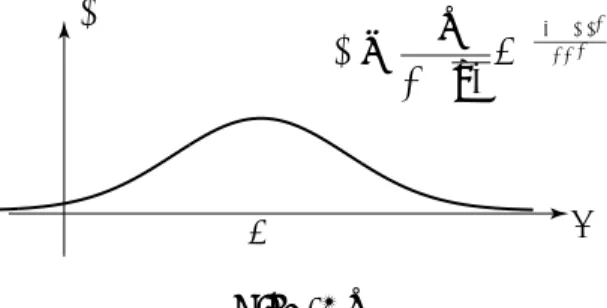
This curve is always ‘bell-shaped’with the centre of the bell located at the value of µ. The depth of the bell is controlled by the value of σ. As with all normal distribution curves it is symmetrical about the centre and decays exponentially as x → ±∞. As with any probability density function the area under the curve is equal to 1. See Figure 1.

y= 1 σ√2πe −(x−µ)2 2σ2 µ x y Figure 1

A normal distribution is completely deﬁned by specifying its mean (the value of µ) and its variance (the value of σ2_{). The normal distribution with mean} _µ _{and variance} _σ2 _{is written}

N(µ, σ2_{). Hence the disribution} _N₍₂₀_,_{25) has a mean of 20 and a standard deviation of 5;}

remember that the second “coordinate” is the variance and the variance is the square of the standard deviation.

The standard normal distribution curve.

At this stage we shall, for simplicity, consider what is known as a standard normal distribution which is obtained by choosing particularly simple values for µand σ.

Key Point

The standard normal distribution has a mean of zero and a variance of one. In Figure 2 we show the graph of the standard normal bistribution which has probability density function y= √1 2π e −x2_/₂ 0 x y y=√1 2π e −x2_/₂

(3)

The result which makes the standard normal distribution so important is as follows:

Key Point

If the behaviour of a continuous random variableXis described by the distributionN(µ, σ2_{) then}

the behaviour of the random variableZ = X_σ−µ is described by the standard normal distribution

N(0,1).

We call Z the standardised normal variable.

Example

If the random variableXis described by the distributionN(45,0.000625) then what is the transformation to obtain the standardised normal variable?

Solution

Here, µ= 45and σ2 _{= 0}_._{000625so that} _σ _{= 0}_._{025. Hence} _Z _{= (}_X₋₄₅₎_/₀_._{025is the required}

transformation.

Example

When the random variable X takes values between 44.95 and 45.05, between which values does the random variable Z lie?

Solution

When X = 45.05, Z = 45₀.05_.₀₂₅−45 = 2 When X = 44.95, Z = 44₀.95_.₀₂₅−45 =−2 Hence Z lies between −2 and 2.

Now do this exercise

The random variable X follows a normal distribution with mean 1000 and variance 100. WhenXtakes values between 1005and 1010, between which values does the standardised normal variableZ lie?

Answer

2. Probabilities and the standard normal distribution

Since the standard normal distribution is used so frequently tables have been produced to help us calculate probabilities. This table is located at the end of this block. It is based upon the following diagram:

0 z1

(4)

Since the total area under the curve is equal to 1 it follows from the symmetry in the curve that the area under the curve in the region x >0 is equal to 0.5. In Figure 3 the shaded area is the probability that Z takes values between 0 and z1.

When we ‘look-up’ a value in the table we obtain the value of the shaded area.

Example

What is the probability that Z takes values between 0 and 1.9?

Solution

The second column headed ‘0’ is the one to choose and its entry in the row neginning ‘1.9’ is 4713. This is to be read as 0.4713 (we omitted the 0 in each entry for clarity) The interpretation is that the probability that Z takes values between 0 and 1.9 is 0.4713.

Example

Solution

This time we want the column headed ‘6’ and the row beginning 1.9. The entry is 4750 so that the required probability is 0.4750.

Example

Solution

There is no entry corresponding to 1.965so we take the average of the values for 1.96 and 1.97. (This linear interpolation is not strictly correct but is acceptable).

The two values are 4750 and 4756 with an average of 4753. Hence the required probability is 0.4753.

What are the probabilities thatZ takes values between

(i) 0 and 2 (ii) 0 and 2.3 (iii) 0 and 2.33 (iv) 0 and 2.333?

Answer Note from the table that as Z increases from 0 the entries increase, rapidly at ﬁrst and then more slowly, toward 5000 i.e. a probability of 0.5. This is consistent with the shape of the curve. After Z = 3 the increase is quite slow so that we tabulate entries for values of Z rising by 0.1 instead of 0.01 as in the rest of the table.

(5)

3. Calculating other probabilities

In this section we see how to calculate probabilities represented by areas other than those of the type shown in Figure 3.

Case 1

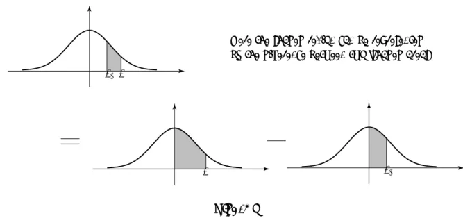
Figure 4 illustrates what we do if both Z values are positive. By using the properties of the standard normal distribution we can organise matters so that any required area is always of ‘standard form’. 0 z1 0 0 z1 z2 z2

Here the shaded region can be represented by the diﬀerence between two ‘shaded areas’

Figure 4

Example

Find the probability that Z takes values bwteen 1 and 2.

Solution

Using the table

P(Z =z2) i.e. P(Z = 2) is 0.4772

P(Z =z1) i.e. P(Z = 1) is 0.3413.

Hence P(1< Z <2) = 0.4772−0.3413 = 0.1359

(Remember that with a continuous distribution, P(Z = 1) is meaningless so thatP(1≤Z ≤2) is also 0.1359.

(6)

Case 2

The following diagram illustrates the procedure to be followed when ﬁnding probabilities of the formP(Z > z1).

0 z1

0 0 z1

This time the shaded area is the diﬀerence between the right-hand half of the total area and a tabulatedﬂ

area 0.5

area.

Figure 5

Example

What is the probability that Z >2?

Solution

P(0< Z <2) = 0.4772 (from the table)

Hence the probability is 0.5−0.4772 = 0.0228.

Case 3

Here we consider the procedure to be followed when calculating probabilities of the

form P(Z < z1). Here the shaded area is the sum of the left-hand half of the total area and a

‘standard’area. 0 z1 0 0 z1 area 0.5 Figure 6

(7)

Example

What is the probability that Z <2?

Solution

P(Z >2) = 0.5 + 0.4772 = 0.9772.

Case 4

Here we consider what needs to be done when calculating probabilities of the form

P(−z1 < Z <0) where z1 is positive. This time we make use of the symmetry in the standard

normal distribution curve.

0

0 z1 −z1

this shaded area is equal in value to the one above.

symmetry by

Figure 7

Example

What is the probability that −2< Z <0?

Solution

(8)

Case 5

Finally we consider probabilities of the form P(−z2 < Z < z1). Here we use the sum property

and the symmetry property.

0 z1 ₀ 0 z2 z2 −z1 Figure 8

Example

What is the probability that −1< Z <2?

Solution

P(−1< Z <0) = P(0< Z <1) = 0.3413

P(0< Z <2) = 0.4772

Hence the required probability, P(−1< Z <2) is 0.8185.

Other cases can be handed by a combination of the ideas already used.

Find the following probabilities.

(i) P(0< Z <1.5) (ii) P(Z >1.8) (iii) P(1.5< Z <1.8) (iv) P(Z <1.8) (v) P(−1.5< Z <0) (vi) P(Z <−1.5) (vii) P(−1.8< Z <−1.5) (viii) P(−1.5< Z <1.8) (A simple sketch of the standard normal curve will help).

(9)

4. Confidence Intervals

We use probability models to make predictions in situations where there is not suﬃcient data available to make a deﬁnite statement. Any statement based on these models carries with it a

risk of being proved incorrect by events.

Notice that the normal probability curve extends to inﬁnity in both directions. Theoretically

any value of the normal random variable is possible, although, of course, values far from the mean position, zero, are very unlikely.

Consider the diagram in Figure 9,

0

−1.96 1.96 95%

Figure 9

The shaded area is 95% of the total area. If we look at the entry in Table 1 corresponding to

Z = 1.96 we see the value 4750. This means that the probability of Z taking a value between 0 and 1.96 is 0.475. By symmetry, the probability thatZ takes a value between −1.96 and 0 is also 0.475. Combining these results we see that

P(−1.96< Z <1.96) = 0.95or 95%

We say that the 95% conﬁdence interval forZ (about its mean of 0) is (−1.96,1.96). It follows that there is a 5% chance that Z lies outside this interval.

We wish to ﬁnd the 99% conﬁdence interval for Z about its mean, i.e. the value of z1 in

Figure 10

0 z1 −z1

99%

Figure 10 The shaded area is 99% of the total area. First, note that 99% corresponds to a probability of 0.99.

Find z1 such that

P(0< Z < z1) =

1

2 ×0.99 = 0.495.

Answer

Now quote the 99% conﬁdence interval.

Answer Notice that the risk of Z lying outside this wider interval is reduced to 1%.

(10)

Find the value of Z

(i) which is exceeded on 5% of occasions (ii) which is exceeded on 99% of occasions.

(11)

Z= x−_σµ 0 1 2 3 4 5 6 7 8 9 0 0000 0040 0080 0120 0160 0199 0239 0279 0319 0359 .1 0398 0438 0478 0517 0577 0596 0636 0675 0714 0753 .2 0793 0832 0871 0909 0948 0987 1026 1064 1103 1141 .3 1179 1217 1255 1293 1331 1368 1406 1443 1480 1517 .4 1555 1591 1628 1664 1700 1736 1772 1808 1844 1879 .5 1915 1950 1985 2019 2054 2088 2123 2157 2190 2224 .6 2257 2291 2324 2357 2389 2422 2454 2486 2517 2549 .7 2580 2611 2642 2673 2703 2734 2764 2794 2822 2852 .8 2881 2910 2939 2967 2995 3023 3051 3078 3106 3133 .9 3159 3186 3212 3238 3264 3289 3315 3340 3365 3389 1.0 3413 3438 3461 3485 3508 3531 3554 3577 3599 3621 1.1 3643 3665 3686 3708 3729 3749 3770 3790 3810 3830 1.2 3849 3869 3888 3907 3925 3944 3962 3980 3997 4015 1.3 4032 4049 4066 4082 4099 4115 4131 4147 4162 4177 1.4 4192 4207 4222 4236 4251 4265 4279 4292 4306 4319 1.5 4332 4345 4357 4370 4382 4394 4406 4418 4429 4441 1.6 4452 4463 4474 4484 4495 4505 4515 4525 4535 4545 1.7 4554 4564 4573 4582 4591 4599 4608 4616 4625 4633 1.8 4641 4649 4656 4664 4671 4678 4686 4693 4699 4706 1.9 4713 4719 4726 4732 4738 4744 4750 4756 4761 4767 2.0 4772 4778 4783 4788 4793 4798 4803 4808 4812 4817 2.1 4821 4826 4830 4834 4838 4842 4846 4850 4854 4857 2.2 4861 4865 4868 4871 4875 4878 4881 4884 4887 4890 2.3 4893 4896 4898 4901 4904 4906 4909 4911 4913 4916 2.4 4918 4920 4922 4925 4927 4929 4931 4932 4934 4936 2.5 4938 4940 4941 4943 4946 4947 4948 4949 4951 4952 2.6 4953 4955 4956 4957 4959 4960 4961 4962 4963 4964 2.7 4965 4966 4967 4968 4969 4970 4971 4972 4973 4974 2.8 4974 4975 4976 4977 4977 4978 4979 4979 4980 4981 2.9 4981 4982 4982 4983 4984 4984 4985 4985 4986 4986 3.0 3.1 3.2 3.3 3.4 3.5 3.6 3.7 3.8 3.9 4987 4990 4993 4995 4997 4998 4998 4999 4999 4999 The Normal Probability Integral

(12)

(13)

The transformation isZ = X−1000 10 .

when X = 1005, Z = ₁₀5 = 0.5 when X = 1010, Z = 10₁₀ = 1.

Hence Z lies between 0.5and 1. Back to the theory

(14)

(i) The entry is 4772; the probability is 0.4772. (ii) The entry is 4803; the probability is 0.4803. (iii) The entry is 4901; the probability is 0.4901. (iv) The entry for 2.33 is 4901, that for 2.34 is 4904.

Linear interpolation gives a value of 4901 + 0.3(4904−4901) i.e. about 4903; the probability is 0.4903.

(15)

(i) 0.4332 (direct from table) (ii) 0.5−0.4641 = 0.0359 (iii) P(0< Z <1.8)−P(0< Z <1.5 ) = 0.4641−0.4332 = 0.0309 (iv) 0.5 + 0.4641 = 0.9641 (v) P(−1.5< Z <0) = P(0< Z <1.5 ) = 0.4332 (vi) P(Z <−1.5 ) =P(Z >1.5 ) = 0.5−0.4332 = 0.0668 (vii) P(−1.8< Z <−1.5 ) =P(1.5< Z <1.8) = 0.0359 (viii)P(0< Z <1.5 ) +P(0< Z <1.8) = 0.8973

(16)

We look for a table value of 4950. The nearest we get is 4949 and 4951 corresponding to

Z = 2.57 andZ = 2.58 respectively. We chooseZ = 2.58 Back to the theory

(17)

(−2.58, 2.58) or −2.58< Z <2.58. Back to the theory

(18)

(i) The value isz1, whereP(Z > z1) = 0.05. Hence P(0< Z < z1) = 0.5−0.05= 0.45This

corresponds to a table entry of 4500. The nearest values are 4495 (Z = 1.64) and 4505 (Z = 1.65).

(ii) Values less than z1 occur on 1% of occasions. By symmetry values greater than (−z1)

occur on 1% of occasions so thatP(0< z <−z1) = 0.49. The nearest table corresponding to

4900 is 4901 (Z = 2.33).

Hence the required value is z1 =−2.33.