Running Time Analysis of ACO Systems
for Shortest Path Problems
Christian Horoba1 and Dirk Sudholt1,2⋆
1
Fakult¨at f¨ur Informatik, LS 2, Technische Universit¨at Dortmund, Dortmund, Germany,[email protected]
2
International Computer Science Institute, Berkeley, USA
Abstract. Ant Colony Optimization (ACO) is inspired by the ability of
ant colonies to find shortest paths between their nest and a food source. We analyze the running time of different ACO systems for shortest path problems. First, we improve running time bounds by Attiratanasunthron and Fakcharoenphol [Information Processing Letters, 105(3):88–92, 2008] for single-destination shortest paths and extend their results for acyclic graphs to arbitrary graphs. Our upper bound is asymptotically tight for large evaporation factors, holds with high probability, and transfers to the all-pairs shortest paths problem. There, a simple mechanism for exchanging information between ants with different destinations yields a significant improvement. Our results indicate that ACO is the best known metaheuristic for the all-pairs shortest paths problem.
1
Introduction
Ant Colony Optimization (ACO) is a rapidly growing field with many applica-tions to problems from combinatorial optimization. It is inspired by the foraging behavior of real ants, which enables an ant colony to find shortest paths be-tween its nest and a food source. Ants communicate by placing pheromone on the ground while searching the environment for food. Other ants are attracted by pheromone trails and therefore tend to follow previous ants. In case foraging ants discover different paths between a nest and a food source, a short path typically gets invested with pheromone more quickly than a longer path. The more ants take the short path, the more pheromone is deposited, until almost all ants follow the short path.
The communication mechanism of real ants has been transferred to many optimization problems such as the TSP [1], routing problems [2, 3], and many other combinatorial problems, see the book by Dorigo and St¨utzle [4]. Despite a plethora of applications, the theoretical knowledge on ACO is still very limited. First theoretical investigations concerned convergence proofs [5] and simplified models of ACO algorithms [6]. In 2006 the first rigorous investigations of the running time of ACO algorithms were presented independently by Gutjahr [7]
⋆Dirk Sudholt acknowledges financial support by a postdoctoral fellowship from the
and Neumann and Witt [8] for the optimization of simple pseudo-Boolean func-tions. The latter authors presented an algorithm called 1-ANT. This algorithm memorizes the best solution found so far. In each iteration a new solution is constructed and the pheromones are updated in case another solution with at least the same quality is found. In other words, every new best-so-far solution is rewarded only once. Investigations of the 1-ANT [8, 9] have shown that if the evaporation strengthρis set too small the algorithm stagnates on even very sim-ple problems and the expected time until an optimum is found is exponential. Other algorithms, variants of the MAX-MIN Ant System (MMAS) [10], reinforce the best-so-far solution in every iteration. This avoids the problem of stagnation and leads to efficient running times on various test problems [11, 12].
Neumann, Sudholt, and Witt [13] investigated the effect of hybridizing ACO with local search. Regarding combinatorial problems, Neumann and Witt [14] presented an analysis for minimum spanning trees. Attiratanasunthron and Fak-charoenphol [15] presented a running time analysis of ACO algorithms on a shortest path problem, the single-destination shortest path problem (SDSP) on directed acyclic graphs (DAGs). Their algorithmn-ANT is inspired both by the 1-ANT [8] and the AntNet algorithm [3]. To our knowledge, this is the first and only rigorous running time analysis for ACO on a shortest path problem. This is surprising as shortest path problems crucially inspired the development of ACO. The aim of this work is to bring forward the theory of ACO for shortest path problems. Shortest paths have already been investigated in the context of other metaheuristics. Scharnow, Tinnefeld, and Wegener [16] presented an analysis of a simple evolutionary algorithm, the (1+1) EA, for the single-source shortest path problem (SSSP). The problems SDSP and SSSP are in essence identical. Their results were later refined by Doerr, Happ, and Klein [17]. In [18] the latter authors investigated a genetic algorithm, simply called GA, for the all-pairs shortest path problem (APSP) and proved that the use of crossover leads to a speed-up com-pared to mutation-based evolutionary algorithms. Finally, Horoba [19] proved that an evolutionary multiobjective algorithm represents a fully polynomial-time approximation scheme for an NP-hard multiobjective shortest path problem. Ta-ble 1 gives an overview on the best known bounds in the single-objective case, including bounds that will be proven in this paper. We remark that problem-specific algorithms solve SDSP for graphs withn vertices andm edges in time O(m+nlogn) and APSP in timeO(nm+n2logn) [20].
In Section 2 we define an ACO algorithm MMASSDSP for the SDSP that differs from then-ANT [15] in two essential ways. Using our modified algorithm we are able to obtain significantly improved running time bounds (see Table 1 and Section 3) and to generalize previous results for DAGs to graphs with cycles. A corresponding lower bound shows that our upper bounds are asymptotically tight if the evaporation factorρis not too small. In Section 4 we transfer these results to a generalized ant system MMASAPSP for the APSP where ants with different destinations move independently. The main result concerns a modifica-tion of MMASAPSPwhere ants temporarily follow foreign pheromone traces. We prove that, surprisingly, this simple mechanism leads to a significant speed-up.
Algorithm Problem Iterations Eval.
n-ANT [15] SDSP on DAGs Om∆ℓlog(∆ℓ)ρ n
MMASSDSP SDSP O ∆ℓℓ∗+ℓlog(∆ℓ) ρ n MMASSDSP SDSP onGlb Ω n2+ n ρlog(1/ρ) n MMASSDSP+adaptiveτmin SDSP O
ℓm+nlogρ n n
(1+1) EA [17] SSSP Θn2ℓ∗ 1
MMASAPSP APSP O
∆ℓℓ∗+ℓlog(∆ℓ) ρ
n2
MMASAPSP+interaction APSP O
nlogn+log(ℓ) log(∆ℓ)ρ n2
GA [18] APSP On3.5√logn 1
Table 1. Overview on the best known running time bounds on graphs with
n vertices, m edges, maximum degree ∆, maximum number of edges ℓ on any shortest path, andℓ∗:= max{ℓ,lnn}. The rightmost column contains the num-ber of path length evaluations in one iteration. The bound for MMASAPSPwith interaction holds forρ≤1/(23∆logn); it simplifies toO(nlog3n) for optimalρ.
2
Algorithms
We consider shortest path problems on weighted directed graphsG= (V, E, w) where w(e) denotes the weight of edgee. The number of vertices is always de-noted by n. We define a path of length ℓ from uto v as a sequence of vertices (v0, . . . , vℓ) where v0 =u,vℓ =v, and (vi−1, vi)∈ E for all i with 1≤i ≤ℓ. For convenience, we also refer to the corresponding sequence of edges as path. Let deg(u) denote the out-degree of a vertex u and ∆(G) denote the max-imum out-degree of any vertex u ∈ V. Let ℓ(G, v) := maxu{#edges onp | pis a shortest path fromuto v}andℓ(G) := maxvℓ(G, v). For undirected non-weighted graphsℓ(G, v) is calledeccentricity of vandℓ(G)diameter ofG.
For the single-destination shortest path problem (SDSP) we are looking for shortest paths from every vertex to a specified destination vertex. The length w(p) of a path pis defined as the sum of weights for all edges in pif the path ends with the destination vertex. If the path does not reach the destination, we define w(p) := ∞. In the following, we only consider positive weights as with negative-length cycles one can find arbitrarily short paths and the problem of computing a shortestsimple path is NP-hard [15].
Attiratanasunthron and Fakcharoenphol [15] present the ACO algorithm n-ANT for the SDSP. Their algorithm is inspired by the 1-ANT [8] and the AntNet routing algorithm [3]. From every vertexu∈V an antaustarts heading for the destination. The path is chosen by performing a random walk through the graph according to pheromones on the edges. Ant au memorizes the best path it has found fromu to the destination so far. If it has found a path that
Algorithm 1Path Construction fromutov for MMASSDSP 1: i←0
2: pi←u
3: V1← {p∈V \ {p0} |(p0, p)∈E}
4: whilepi6=v andVi+16=∅do
5: i←i+ 1
6: choosepi∈Vi with probabilityτ((pi−1, pi))/Pp∈Viτ((pi−1, p))
7: Vi+1← {p∈V \ {p0, . . . , pi} |(pi, p)∈E}
8: end while
9: return (p0, . . . , pi)
is at least as good as the previous best-so-far path, a pheromone update takes place and the new path is reinforced. The authors use a purely local update rule: each antauis responsible for updating the edges leaving its start vertexu. If the new path is worse, the pheromones on the edges leavinguremain unchanged.
As the authors only consider acyclic graphs, then-ANT is not supposed to deal with cycles. In particular, in [15] the authors state that in graphs with cycles their path construction procedure might take exponential time. Therefore, here we only allow ants to construct simple paths, i. e., an ant cannot visit a vertex more than once. The choice which edge to take next is made among all edges leading to unvisited vertices. This restriction bears the risk that the ant does not reach the destination. Recall that in this case the length of the path found is defined as w(p) = ∞. Due to the local pheromone update it is guaranteed that still one outgoing edge is rewarded for every vertexuwith deg(u)≥1 and u6=n. The construction procedure is described in Algorithm 1.
We call our algorithm MMASSDSPas we use the best-so-far update rule from the algorithm MMAS in [12] instead of the update rule used by the 1-ANT. The difference is that we always perform a pheromone update with the current best-so-far path, either with a new path or with the previous best-best-so-far path in case the new path is worse.
The update scheme is essentially taken over from [15]. We initialize the pher-omones τ:E→R+0 such that all edges leaving some vertexureceive the same
amount of pheromone: if e= (u,·) then τ(e) = 1/deg(u). If eis the only edge leaving u, we keep τ(e) = 1 fixed. This means that vertices with a single out-going edge are traversed in the only possible way; these vertices may therefore be disregarded when proving upper bounds on the running time. In caseuhas more than one outgoing edge, the pheromone for e= (u, v) is computed as fol-lows. Let p∗
u denote the best path from u found so far. Initially, we set p∗u to an empty path, which has infinite length by definition of w. As in [10, 15] we use pheromone borders to keep pheromones within an interval [τmin, τmax]. In a pheromone update then
τ(e)← (
min{(1−ρ)·τ(e) +ρ, τmax} ife= (u, v)∈p∗u, max{(1−ρ)·τ(e), τmin} ife= (u, v)∈/p∗u.
Algorithm 2MMASSDSP
1: initialize pheromonesτ and best-so-far pathsp∗ 1, . . . , p∗n 2: loop
3: foru= 1 tondo
4: construct a simple pathpu= (pu,0, . . . , pu,ℓu) fromutonw. r. t.τ
5: if w(pu)≤w(p∗u)thenp∗u←pu end if
6: end for
7: update pheromonesτ w. r. t.p∗ 1, . . . , p∗n
8: end loop
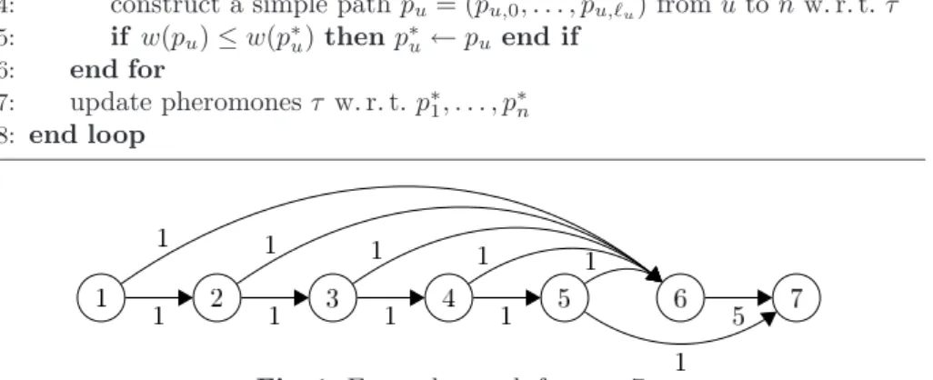
Fig. 1. Example graph forn= 7.
The complete algorithm is shown in Algorithm 2. We are interested in the
optimization timeorrunning time of MMASSDSP, i. e., the number of iterations until shortest paths from 1, . . . , nto nhave been found. Another common per-formance measure for metaheuristics is the number of function evaluations. Note that in one iteration of MMASSDSPwe havenants constructingnsolutions and performing n function evaluations in parallel. Hence, the number of function evaluations is by a factornlarger than the number of iterations.
Before analyzing MMASSDSP we motivate why it is essential to have ants starting from every vertex, even when we are only interested in the shortest path from a single source to a single destination and even when considering simple DAGs. Imagine a variant MMASSPSP(SPSP for single-pair shortest paths) where one or multiple ants start from a single vertex, searching for the destination. Consider the following graph G = (V, E, w) sketched in Figure 1. It contains a single heavy edge (n−1, n) with weight n−2 and light edges (u, n−1) for u≤n−2, (u, u+ 1) foru≤n−3 and (n−2, n) of weight 1, each.
On each vertex u≤n−2 an ant has to decide whether to move to n−1 or to proceed on the shortest path. As all edges initially have equal pheromone, the probability that an ant follows the shortest path to vertex n/2 is 2−n/2+1. Assume the ant leaves the shortest path before reachingn/2. As the length of a path containingℓedges and traversingn−1 isℓ+n−3, no further path with a larger number of edges will be accepted in the following, except for the optimal path traversing 1,2, . . . , n−2, n. This implies that the pheromones for edges leaving the verticesn/2, . . . , n−2 will always remain equal, unless an ant finds the optimum. The probability of finding the optimum is 2−n/2+1, hence taking the union bound over 2cnsteps for some small constantc >0, the optimization time is at least 2cnwith probability 1
−2−Ω(n). Note that this also holds in case polynomially many ants search for the destination in parallel in one iteration.
Also using edge weights as heuristic information does not help. Many ACO algorithms use both pheromones and a heuristic function to guide the solution construction [4]. However, from a vertex n/2≤u≤n−2 both outgoing edges have the same weight and the same pheromone, with high probability, hence they look the same for every ant. This example also shows that heuristic information may be useless or even misleading for some problem instances.
3
Single-Destination Shortest Path Problem
When ants start from different vertices, ants starting close to the destination have a good chance of finding a shortest path. The pheromones deposited on the outgoing edges of a vertexvcan then be used to guide different ants traversingv. This way, the shortest path forvcan be extended towards a longer shortest path that containsv. This is the basic idea of the analysis by Attiratanasunthron and Fakcharoenphol [15], which is improved and generalized in this section. Their results are limited to directed acyclic graphs. We start with these graphs and extend the results to directed graphs with cycles.
Lemma 1. If τmin+τmax= 1 then for every vertex uwithdeg(u)>1 always
1 ≤ X
e=(u,·)∈E
τ(e) ≤ 1 + deg(u)τmin.
Proof.The first inequality has already been proven in [15]. Initially the sum of
pheromones equals 1. Assume for an induction that Pτ(e)
≥1. If the phero-mones are not capped by pheromone borders, we have (1−ρ)Pτ(e) +ρ
≥1 as new sum. In case a pheromone drops belowτmin, setting the pheromone toτmin can only increase the sum. If at least one pheromone is capped at the upper bor-derτmax then the sum of pheromones is at leastτmin+τmax= 1 as deg(u)>1. For the second inequality observe that the sum of pheromones can only in-crease due to the lower pheromone border as (1−ρ)P
τ(e) +ρ≤P
τ(e) follows fromP
τ(e)≥1. Consider an edgeewith (1−ρ)τ(e)< τmin. Compared to this value, the pheromone increases by at mostτmin·ρwhen setting the pheromone toτmin. If currentlyPτ(e)≤1+deg(u)τminthen the sum of the next pheromone values is at most (1−ρ)(1 + deg(u)τmin) +ρ+ deg(u)τmin·ρ = 1 + deg(u)τmin.
Hence, the second inequality follows by induction.
As an immediate consequence, we obtain the following direct relation be-tween pheromones and probabilities for the antau, i. e., the ant starting atu, of choosing an edge (u,·) in caseτmin≤1/deg(u). The last condition makes sense asτmin should be chosen below the initial pheromone value of 1/deg(u).
Corollary 1. Ifτmin≤1/deg(u)andτmin+τmax= 1 for every edgee= (u,·)
τ(e)/2 ≤ Prob(antau chooses edgee) ≤ τ(e).
The lower bound also holds for every other ant leaving vertex uand every edge
holds for every other ant and every edge e = (u,·) if it has not traversed a successor ofubefore arriving at u.
The penultimate statement holds as the probability of choosing an edgee= (u, v) to an unvisited successor v increases if other successors ofu have been visited before. In particular, we always haveτmin/2 as lower bound on the probability of choosing any specific outgoing edge. This is an improvement to Lemma 1 in [15]. We remark that using the improved lemma in [15], the running time bounds for the algorithmn-ANT can be divided bym/n, wheremis the number of edges. The following theorem gives upper bounds for MMASSDSP, each consisting of two additive terms. Intuitively, the first terms cover waiting times until im-provements of best-so-far paths are found. The second terms grow with 1/ρ. They reflect the time to adapt the pheromones after a change of the best-so-far path. This time is calledfreezing time by Neumann, Sudholt, and Witt [12].
Theorem 1. Consider a directed acyclic graph G with n vertices and positive
weights. The expected optimization time of MMASSDSP onG withτmin:= 1/n2
and τmax = 1−τmin isO(n3+ (nlogn)/ρ). Let ∆ := ∆(G) and ℓ :=ℓ(G, n).
The expected optimization time of MMASSDSP with τmin= 1/(∆ℓ) andτmax = 1−τmin isO(n∆ℓ+nlog(∆ℓ)/ρ).
Proof.We follow the analysis by Attiratanasunthron and Fakcharoenphol [15].
Call an edge (u, v) incorrect if it does not belong to any shortest path fromu ton. We say that a vertexuisprocessed if a shortest path fromutonhas been found and if all incorrect edges leavinguhave pheromoneτmin.
We estimate the expected time until a vertexu has been processed, given that all vertices reachable from u on shortest paths from uto n have already been processed. We first consider the expected time until a shortest path fromu ton has been found for the first time. We also say that then vertexuhas been
optimized. By Corollary 1 the probability of choosing an edge that belongs to a shortest path from u to n is at least τmin/2. Such a shortest path is found if the ant does not choose an incorrect edge until n is reached. As all vertices on all shortest paths are processed, all incorrect edges at some vertex v have pheromoneτmin and the probability of choosing some incorrect edge is at most deg(v)τmin. Hence, the probability of choosing an edge on a shortest path is at least 1−deg(v)τmin ≥1−1/ℓ if τmin ≤1/(deg(v)ℓ). As all shortest paths have at most ℓ edges, the probability that no incorrect edge is chosen is at least (1−1/ℓ)ℓ−1≥1/ewith e= exp(1). Together, the probability of finding a shortest path fromutonis at leastτmin/(2e).
The expected time untiluis optimized is thus at most 2e/τmin. Afterwards, due to the best-so-far rule, a shortest path from uton is reinforced automati-cally in each iteration. The precise path may change, but it is guaranteed that only shortest paths are rewarded and hence the pheromone on incorrect edges decreases in every step. Lemma 2 in [15] states that ln(τmax/τmin)/ρiterations are enough for the vertex to become processed, hence the expected time untilu is processed is bounded by 2e/τmin+ ln(τmax/τmin)/ρ.
Letv1, . . . , vn−1 be an enumeration of the vertices in V \ {n} ordered with respect to increasing length of the shortest path ton. As all weights are positive, all shortest paths fromvi+1tononly use vertices from{n, v1, . . . , vi}. Ifv1, . . . , vi have been processed then we can wait for vi+1 to become processed using the above argumentation. The expected time until all verticesv1, . . . , vn−1have been processed is bounded by n2e/τmin+nln(τmax/τmin)/ρ. Choosing τmin := 1/n2 andτmax= 1−τmin, we obtain the boundO(n3+ (nlogn)/ρ). Choosingτmin:= 1/(∆ℓ) andτmax= 1−τminyields the boundO(n∆ℓ+nlog(∆ℓ)/ρ). Observe that for MMASSDSP, once a shortest path from u has been found, the pheromones are continuously “frozen” towards shortest paths fromuin the followingF= ln(τmax/τmin)/ρiterations. The algorithmn-ANT from [15], how-ever, only updates pheromones in case a new best-so-far path is found. This implies that a shortest path fromuhas to be found several times, in the worst case in F different iterations, in order to freeze the pheromones in the same way. Hence, using the best-so-far rule of MMAS algorithms leads to better per-formance results. This adds to the comparison of the 1-ANT and MMAS on pseudo-Boolean problems in [12].
We proceed by improving Theorem 1 in several respects. First, the bound on the expected optimization time is improved at least by a factor of ℓ∗/n. Second, the result not only holds for directed acyclic graphs but for all directed graphs with positive weights and unique shortest paths. Finally, we show that the running time bounds hold with high probability (i. e. with probability at least 1−n−c for some c > 0). In the proof we follow ideas from [17] showing that the random time until a short path of lengthℓ=Ω(logn) is found is highly concentrated around the expectation.3
Theorem 2. Consider a directed graph G with n vertices and positive weights
where all shortest paths are unique. Let ∆ := ∆(G), ℓ := ℓ(G, n), and ℓ∗ := max{ℓ,lnn}. The optimization time of MMASSDSP on G with τmin = 1/(∆ℓ)
andτmax= 1−τmin isO(∆ℓℓ∗+ℓlog(∆ℓ)/ρ)with probability at least 1−1/n2.
The optimization time bound also holds in expectation.
Proof.When estimating the probability that an ant chooses an edge on a
short-est path the lower bound from Corollary 1 always holds. In the proof of Theo-rem 1 we have shown that for antau the probability of finding a shortest path fromuton, given that all successors ofuon shortest paths have been processed, is bounded below by τmin/(2e) if τmin ≤1/(∆ℓ). This result also holds in the case of arbitrary directed graphs.
Fix a vertexuand the unique shortest pathu=vℓ′, vℓ′−1, . . . , v0 =n with ℓ′ ≤ℓ. We pessimistically estimate the expected time untiluis processed. LetT
i be the random time untilviis optimized. Consider random variablesX1, . . . , XT
3
There is a subtle difference to [17]: in their definition ofℓthe authors only consider shortest pathswith a minimum number of edges (if there are several shortest paths between two vertices). Both definitions forℓare, however, equal if all shortest paths
that are independently set to 1 with probability τmin/(2e) and to 0 otherwise. The random first point of time T∗
1 where Xt = 1 stochastically dominates the random time untilv1 is optimized. Asv1becomes processed after an additional waiting time ofF := ln(τmax/τmin)/ρsteps,T1∗+F stochastically dominatesT1. Inductively, we have that T∗
ℓ′+ℓ′F stochastically dominatesTℓ′ and hence the time untiluis processed.
LetT := 16eℓ∗/τ
minandX:=PTi=1Xi. We have E(X) =T·τmin/(2e) = 8ℓ∗. By Chernoff bounds [21]
Prob(X < ℓ∗) ≤ Prob(X ≤(1−7/8)·E(X)) ≤ e−8ℓ∗(7/8)2/2
< e−3ℓ∗ ≤n−3. Hence, the probability thatuis not processed afterT+ℓln(τmax/τmin)/ρsteps is 1/n3. By the union bound, the probability that there is an unprocessed vertex remaining after this time is at most 1/n2. The result on the expectation follows from the first result, which holds for arbitrary initial pheromones. If the algo-rithm does not find all shortest paths within the firstT+ℓln(τmax/τmin)/ρsteps, we repeat the argumentation with another phase of this length. The expected
number of phases needed is clearlyO(1).
3.1 Lower Bounds for MMASSDSP
We now turn to lower bounds on the expected optimization time of MMASSDSP. We begin with a general lower bound, which holds for a wide range of graphs, including most acyclic graphs. The main idea is that the pheromones need some time to adapt, such that a shortest path with ℓ edges can be found with good probability. On the one hand, the bound grows with 1/ρif ρ is not too small. On the other hand, it also applies to pure random search, i. e., ρ= 0.
Theorem 3. Consider a directed acyclic graph G with n vertices and positive
weights. Assume that G contains a unique shortest path p0, . . . , pℓ = n such
that for 0 ≤ i < ℓ we have deg(pi) ≥ 2 and no edges leading back from pi
to {p0, . . . , pi−1}. Let ∆ := ∆(G) and ℓ := ℓ(G, n). If ρ ≤ 1−Ω(1) then the
expected optimization time of MMASSDSP onGwith τmin≤1/(∆ℓ)andτmax= 1−τmin isΩ(min{(logℓ)/ρ, e
√ ℓ/4
}).
Proof.Initially all pheromones on edges (u,·) equal 1/deg(u). During the first
t:= min{(1/ρ−1)·ln(ℓ)·1/2, e√ℓ/4/2
}=Ω(min{(logℓ)/ρ, e√ℓ/4
}) steps (using 1/ρ−1 = Ω(1) by assumption on ρ) the pheromone on every such edge is at least 1 deg(u)·(1−ρ) t ≥deg(u)1 ·e−ln(ℓ)·1/2= 1 deg(u)· 1 √ ℓ.
Note that this even holds in case the lower pheromone border is hit. Consider the ant starting atp0 trying to createp0, . . . , pℓ. As the probability of taking a specific incorrect edge is at leastp:= 1/(2 deg(u)√ℓ), the probability that the ant takes a correct edge on the path is at most 1−(deg(u)−1)·p= 1−(deg(u)−1)· 1/(2 deg(u)√ℓ)≤1−1/(4√ℓ). The probability that the pathp0, . . . , pℓis created
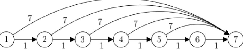
Fig. 2.Example graphGlb from Definition 1 forn= 7.
in a specific iteration t′ ≤ t is hence bounded by (1−1/(4√ℓ))ℓ
≤ e−√ℓ/4. The probability that this happens during the first t iterations is bounded by t·e−√ℓ/4 ≤1/2 due to the definition of t. Hence with probability at least 1/2 we have not found all shortest paths after t steps and the lower bound t/2 = Ω(min{(logℓ)/ρ, e√ℓ/4
}) follows.
In order to assess whether the upper bound from Theorem 2 is asymptotically tight, we consider the following input instance (see Figure 2). The basic idea is that the algorithm is forced to optimize the vertices one after another, from right to left.
Definition 1. Let Glb = (V, E, w) with V ={1, . . . , n}, E = {(i, i+ 1)| 1 ≤
i≤n−1} ∪ {(i, n)|1≤i≤n−2}, and weights w((u, v)) = 1 if v=u+ 1 and
w((u, v)) =n ifv6=u+ 1.
Theorem 2 yields an upper boundO(n2+ (nlogn)/ρ) forG
lb. The following lower bound is tight with the upper bound if ρ =Ω((logn)/n). For smaller ρ there is a gap ofO(log2n).
Theorem 4. If 1/poly(n) ≤ ρ ≤ 1/2 then the expected optimization time of
MMASSDSPonGlbwithτmin= 1/(2n)andτmax= 1−τminisΩ
n2+ n ρlog(1/ρ)
.
Proof. Consider all paths from u to n with u ≤ n−2. The path (u, n) has
lengthn. All other paths start with the edge (u, u+ 1). The length of the path only traversing edges with weight 1 isn−u. However, if the path ends with an edge (v, n) foru < v≤n−2, the path has lengthv−u+n > n. Hence the path (u, n) is the unique second best path fromuton.
Call a vertex u ≤ n−2 wrong if the best-so-far path found by ant au is (u, n). After initialization both edges have an equal probability of being chosen by the first ant. By Chernoff bounds at leastn/3 antsau withu≤n−2 choose incorrect edges with probability 1−e−Ω(n)and then the edges remain incorrect until a shortest path has been found. We assume that we initially haven/3 wrong vertices. First, we show that with high probability after F := ln(τmax/τmin)/ρ iterations we still haven/3−O(log2n) wrong vertices. For these verticesuthe pheromones then are frozen towards the incorrect edge.
As long as a vertex uremains wrong, the pheromone on its correct edge is at most 1/2. (It even decreases continuously towardsτminunless a shortest path is found.) Fix the set of r := 8 log(1/ρ) wrong vertices with largest index and letube the vertex with the smallest index in this set. During a phase comprising the followingt:= 1/ρ−1 steps the probability of choosing the correct outgoing
edge is for each vertex bounded from above by 1−1 4(1−ρ)
t
≤ 1− 1 4e using Corollary 1. The probability that a shortest path for uis found throughout the phase is at mostt(1− 1 4e) r ≤2log(1/ρ)(1 − 1 4e) 8 log(1/ρ) ≤1/2.
We conclude that the time until all r vertices have found shortest paths is at least t with probability at least 1/2 and the expectation is Ω(t). We may repeat these arguments with a new phase and another set of r vertices which are still wrong at that time and have maximal index. Consider 3F/t=Θ(logn) subsequent phases. Applying Chernoff bounds to random variables indicating whether a phase has found shortest paths for the consideredr vertices withint iterations, with high probabilityF/tphases each need at leasttiterations. Hence, with high probability afterFsteps at mostO(logn)·r=O(log2n) wrong vertices have found shortest paths. It may happen that during a phase some vertices preceding therconsidered vertices find shortest paths by chance. However, the probability that a vertexvfinds a shortest path if the path still contains 3 logn+ log(1/ρ) wrong vertices is at most 2−3 logn−log(1/ρ)
≤ ρ/n3. Taking the union bound for at most n vertices andF iterations, this does not happen within F iterations, with high probability. Hence, we correct at most 3 logn+ log(1/ρ) = O(logn) wrong vertices per phase andO(log2n) wrong vertices in total this way. With high probability we obtain a situation where forn/3−O(log2n) wrong vertices pheromones are frozen towards the incorrect edge. We separately prove lower boundsΩ(n/(ρlog(1/ρ))) andΩ(n2) for the expected remaining optimiza-tion time.
The first bound follows from applying the above arguments on phases to the remainingΩ(n) wrong vertices, along with the fact that the probability of finding a shortest path containing i wrong vertices has decreased to (τmin)i ≤ 1/ni. Hence, with high probability at most a constant number of wrong vertices is corrected unexpectedly per phase and the expected time to completeΩ(n/r) = Ω(n/log(1/ρ)) phases yields the first bound.
For the second bound Ω(n2) we observe that the expected time to find a shortest path for u if the path contains at least four wrong vertices is at most (τmin)4 ≤ 1/n4. Hence, with high probability during Ω(n2) iterations it does not happen that more than 4 wrong vertices are corrected in the same iter-ation. The expected time until the wrong vertex with largest index is corrected is 1/τmin≥n. If the number of wrong vertices always decreases by at most 4, the expected time to correctΩ(n) wrong vertices isΩ(n2).
3.2 An Adaptive Choice of Pheromone Borders
The probability of constructing a shortest path fromu, given that all successors of u on shortest paths have been processed, is bounded below by τmin/(2e) if τmin≤1/(deg(u)ℓ). This suggests to chooseτmin as large as possible. However, if the same pheromone borders apply to all edges, the best feasible choice is τmin= 1/(∆ℓ).
It thus makes sense to consider an ACO system where pheromone bor-ders can be adapted to single vertices. The pheromone on an edge e = (u,·) is then bounded by the pheromone borders τmin(u) and τmax(u). If τmin(u) =
1/(deg(u)ℓ) andτmax(u) = 1−τmin(u) then the expected waiting time untiluis optimized, given that all successors on shortest paths are processed, is bounded by 2e/τmin(u) = 2edeg(u)ℓ. The adaptation leads to the following bound.
Theorem 5. Consider a directed graphGwithnvertices,medges, and positive
weights. Let ℓ :=ℓ(G, n). The expected optimization time of MMASSDSP using
adaptive pheromone borders with τmin(u) = 1/(deg(u)ℓ) and τmax(u) = 1− τmin(u)for all verticesuisO(ℓm+ (nlogn)/ρ).
4
All-Pairs Shortest Path Problem
We now extend MMASSDSPtowards an algorithm MMASAPSPfor the APSP. For each destinationv∈V we introduce a distinct pheromone functionτv:E→R+0. In each iteration, on each vertexu, and for each destinationvwe have an antau,v starting atuand heading for v. An ant heading forv uses the pheromone func-tionτv for orientation and it updatesτv as described in Section 2. MMASAPSP remembers the best-so-far pathp∗
u,v fromutov for allu, v∈V. The following result is an immediate implication from Theorem 2.
Theorem 6. Consider a directed graph G with nvertices and positive weights
where all shortest paths are unique. Let ∆ := ∆(G) and ℓ :=ℓ(G). The opti-mization time of MMASAPSPon G withτmin= 1/(∆ℓ) andτmax = 1−τmin is O(∆ℓℓ∗+ℓlog(∆ℓ)/ρ) with probability at least 1−1/n. The optimization time
bound also holds in expectation.
We see that ants heading for different destinations do not collaborate in our ant system since ants heading for a destination v concern for the pheromone functionτv exclusively. Therefore we could also runninstances of MMASSDSP in parallel to achieve the same result. An obvious question is whether the ants can interact in some clever way to achieve a better result.
Interestingly, the following very simple mechanism proves useful. Consider the ant au,vheading for vertexv. Instead of always using the pheromone func-tionτv to travel tov, with probability, say, 1/2 the ant decides to follow foreign pheromones. It first chooses an intermediate destination w uniformly at ran-dom, then uses the pheromone function τw to travel to w, and afterwards uses the pheromone functionτvto travel to the final destinationv(see Algorithm 3). The pheromone update for antau,valways applies to the pheromonesτv.
With this mechanism the ant au,v can profit from useful information laid down by other ants that headed towards w, in particular ifw happens to be a vertex on a shortest path fromutov. The following theorem gives a significantly improved bound, without restriction to graphs with unique shortest paths.
Theorem 7. Consider a directed graphGwith nvertices and positive weights.
Let ∆:=∆(G),ℓ:=ℓ(G), andℓ∗:= max{ℓ,lnn}. Ifρ≤1/(23∆logn)then the
optimization time of MMASAPSPusing interaction onGwithτmin= 1/(∆ℓ)and τmax= 1−τminisO(nlogn+ log(ℓ) log(∆ℓ)/ρ)with probability at least1−1/n2.
Algorithm 3Path construction fromutov for MMASAPSP with interaction 1: if getRandomBit() = 0 then
2: construct a simple pathpfromutov w. r. t.τv 3: else
4: choosew∈V uniformly at random 5: construct a simple pathp′ = (p′
0, . . . , p′ℓ′) fromuto ww. r. t.τw 6: construct a simple pathp′′= (p′′
0, . . . , p′′ℓ′′) from wtov w. r. t.τv 7: if p′
ℓ′ =wthenp←(p′0, . . . , p′ℓ′, p′′1, . . . , p′′ℓ′′)else p←p′ end if
8: end if
9: return p
Proof.We introduce similar notions as before. Consider a pair (u, v) of vertices.
Let ℓu,v denote the maximum number of edges of a shortest path fromuto v. We call an edge incorrect with respect to v if it does not belong to a shortest path tov. We call (u, v)optimized if a shortest path fromutovhas been found. We call (u, v)processed if it has been optimized and if the pheromoneτv(·) on all incorrect edges (u,·) isτmin.
Consider the first t = (ln 2)/ρ = O(1/ρ) iterations. Consider a pair (u, v) with ℓu,v = 1. The probability of optimizing (u, v) in iteration i is at least (1−ρ)i−1/(4∆) since the ant a
u,v decides with probability 1/2 to head for v and chooses (u, v) with probability at least (1−ρ)i−1/(2∆) due to Corollary 1. Hence, the probability ofnot optimizing (u, v) within the considered phase is at most t Y i=1 1−(1−ρ) i−1 4∆ ≤exp − 1 4∆ t−1 X i=0 (1−ρ)i ! = exp −1−(1−ρ) t 4∆ρ .
Since ρ ≤ 1/(23∆logn) ≤ 1/(8∆ln(2n4)), the above probability is at most 1/(2n4). Because of the union bound, all pairs (u, v) withℓ
u,v= 1 are optimized within the considered phase with probability at least 1−f1wheref1:= 1/(2n2). We know that an optimized pair (u, v) is processed within ln(τmax/τmin)/ρ iter-ations.
Consider a pair (u, v) and fix a shortest pathpu,vfromutovwithℓu,vedges. Let iwith (3/2)i < ℓ
u,v ≤(3/2)i+1. If all pairs (u′, v′) withℓu′,v′ ≤(3/2)i are processed, the probability of optimizing (u, v) is at least 1/2·ℓu,v/(3n)·1/e > (3/2)i/(6en) since the ant decides with probability 1/2·ℓ
u,v/(3n) to choose an intermediate destinationwon the middle third ofp. Hence, the number of edges of all shortest paths pu,w (pw,v) from u (w) to w (v) is at most (3/2)i. Since (x, w) ((x, v)) is processed for all vertices xon a shortest path from u (w) to w (v), the ant follows a shortest path from u to v with probability at least (1−1/ℓ)ℓ−1
≥1/e.
We divide a run of the ant system into phases. Theith phase finishes with all pairs (u, v) with (3/2)i−1< ℓ
u,v≤(3/2)i being processed. Sinceℓu,v≤ℓ, we have to considerα:=⌈log(ℓ)/log(3/2)⌉phases.
Consider Phasei of length t= 6en/(3/2)iln(2αn4). The probability of not optimizing a pair (u, v) with (3/2)i−1 < ℓ
u,v ≤ (3/2)i within the phase is at most (1−(3/2)i/(6en))t
≤ 1/(2αn4). Due to the union bound, all such pairs (u, v) are optimized withintiterations with probability at least 1−1/(2αn2). We know that an optimized pair (u, v) is processed within ln(τmax/τmin)/ρiterations. Using the union bound, all phases are finished within
α X i=1 6enln(2αn4) (3/2)i + ln(∆ℓ) ρ ≤6enln(2αn4) α X i=1 2 3 i +αln(∆ℓ) ρ =O(nlogn+ log(ℓ) log(∆ℓ)/ρ)
iterations with probability at least 1−f2 where f2 := 1/(2n2). The first part of the theorem follows since both failure probabilities f1 and f2 sum up to 1/n2. The second part can be derived using the bound O(n3+ (nlogn)/ρ) on the expected optimization time. This bound can be easily shown for all graphs (without restriction to unique shortest paths) using ideas from the proofs of
Theorems 1 and 2.
We remark that the choice of the probability 1/2 for choosing an intermediate vertex is not essential; using any other constant value 0< p <1 would only affect the constants in Theorem 7. If ∆, ℓ = Ω(n) and ρ = 1/(23∆logn) the upper bounds given in Theorem 6 and Theorem 7 simplify toO(n3) andO(nlog3n), respectively. Hence, the ant system clearly profits from our simple interaction mechanism and more collaboration between the ants.
5
Conclusions
ACO is motivated by the ability of real ant colonies to find shortest paths to a food source. Building on an initial study by Attiratanasunthron and Fakchar-oenphol [15], we have conducted a rigorous analysis of the running time of ACO algorithms for shortest path problems. Our results (see Table 1) significantly improve and generalize the previous results for single-destination shortest paths. Taking the number of function evaluations as performance measure, the bound for MMASSDSP is better than the bound for the (1+1) EA [17] if∆ℓ=o(n) and ρis not too small.
For all-pairs shortest paths first results have been obtained using MMASAPSP as a direct generalization of MMASSDSP. We have proved that, surprisingly, letting ants temporarily follow foreign pheromone traces to random destinations yields drastically improved results. This is also the first result for combinatorial optimization where a slow adaptation for pheromones is crucial, i. e., low values for the evaporation factorρyield the best upper bounds. For an optimal choice of ρ the bound of O(n3log3n) function evaluations improves upon the best known bound O(n3.5√logn) for genetic algorithms [18]. This makes ACO the currently best known metaheuristic for the all-pairs shortest path problem from a theoretical perspective.
References
[1] Dorigo, M., Gambardella, L.M.: Ant colony system: A cooperative learning ap-proach to the traveling salesman problem. IEEE Transactions on Evolutionary Computation1(1) (1997) 53–66
[2] Dorigo, M., Maniezzo, V., Colorni, A.: The ant system: An autocatalytic opti-mizing process. Technical Report 91-016 Revised, Politecnico di Milano (1991) [3] Di Caro, G., Dorigo, M.: AntNet: Distributed stigmergetic control for
communi-cations networks. Journal of Artificial Intelligence Research9(1998) 317–365 [4] Dorigo, M., St¨utzle, T.: Ant Colony Optimization. MIT Press (2004)
[5] Gutjahr, W.J.: A generalized convergence result for the graph-based ant sys-tem metaheuristic. Probability in the Engineering and Informational Sciences17
(2003) 545–569
[6] Merkle, D., Middendorf, M.: Modelling the dynamics of Ant Colony Optimization algorithms. Evolutionary Computation10(3) (2002) 235–262
[7] Gutjahr, W.J.: First steps to the runtime complexity analysis of ant colony opti-mization. Computers and Operations Research35(9) (2008) 2711–2727
[8] Neumann, F., Witt, C.: Runtime analysis of a simple ant colony optimization algorithm. In: Proc. of ISAAC ’06, Springer (2006) 618–627
[9] Doerr, B., Neumann, F., Sudholt, D., Witt, C.: On the runtime analysis of the 1-ANT ACO algorithm. In: Proc. of GECCO ’07, ACM Press (2007) 33–40 [10] St¨utzle, T., Hoos, H.H.: MAX-MIN ant system. Journal of Future Generation
Computer Systems16(2000) 889–914
[11] Gutjahr, W.J., Sebastiani, G.: Runtime analysis of ant colony optimization with best-so-far reinforcement. Methodology and Computing in Applied Probability
10(2008) 409–433
[12] Neumann, F., Sudholt, D., Witt, C.: Analysis of different MMAS ACO algorithms on unimodal functions and plateaus. Swarm Intelligence3(1) (2009) 35–68 [13] Neumann, F., Sudholt, D., Witt, C.: Rigorous analyses for the combination of
ant colony optimization and local search. In: Proc. of ANTS ’08, Springer (2008) 132–143
[14] Neumann, F., Witt, C.: Ant Colony Optimization and the minimum spanning tree problem. In: Proc. of LION ’07, Springer (2008) 153–166
[15] Attiratanasunthron, N., Fakcharoenphol, J.: A running time analysis of an ant colony optimization algorithm for shortest paths in directed acyclic graphs. In-formation Processing Letters105(3) (2008) 88–92
[16] Scharnow, J., Tinnefeld, K., Wegener, I.: The analysis of evolutionary algorithms on sorting and shortest paths problems. Journal of Mathematical Modelling and Algorithms3(4) (2004) 349–366
[17] Doerr, B., Happ, E., Klein, C.: A tight analysis of the (1+1)-EA for the single source shortest path problem. In: Proc. of CEC ’07, IEEE Press (2007) 1890–1895 [18] Doerr, B., Happ, E., Klein, C.: Crossover can provably be useful in evolutionary
computation. In: Proc. of GECCO ’08, ACM Press (2008) 539–546
[19] Horoba, C.: Analysis of a simple evolutionary algorithm for the multiobjective shortest path problem. In: Proc. of FOGA ’09, ACM Press (2009) 113–120 [20] Cormen, T.H., Leiserson, C.E., Rivest, R.L., Stein, C.: Introduction to
Algo-rithms. 2nd edn. The MIT Press (2001)
[21] Mitzenmacher, M., Upfal, E.: Probability and Computing. Cambridge University Press (2005)