Vol 8, No 9 (2019)

(1)

DETERMINATION OF THE BEST PROBABILITY

DISTRIBUTION OF FIT FOR OZONE CONCENTRATION DATA

IN CAMPO GRANDE-MS-BRAZIL

Amaury de Souza,

[a]*

Bulbul Jan,

[b]

Faisal Nawaz,

[c]

Muhammad Ayub Khan

Yousuf Zai,

[d]

_{Hamilton G. Pavao,}

[a]

_{Widnei A. Fernandes,}

[a]

_{Soetânia Santos de Oliveira,}

[d]

_Ivana

Pobocikova,

[e]

Jane Rose Leite Larréa Seabra,

[a]

Marcel Carvalho Abreu,

[f]

José Francisco de

Oliveira Júnior,

[h]

Gabrielly Cristhine Zwang Baptista

[i]

Keywords:ozone, probability distribution, fit quality tests.

This study discussed the behavior of ozone level observed in the atmospheric region of Campo Grande. To determine the best adjusted distribution to describe the ozone co-generation data for the year 2016 in Campo Grande were used 15 functions adjusted for this purpose; the performances of the distributions are evaluated using three test qualities, namely Kolmogorov- Smirnov, Anderson-Darling and Chi-Square test. Finally, the result of the fitted quality test is compared, it was observed that the generalized extreme value distribution provides a good fit for the whole year and the distributions Gamma 3P; lognormal 3P; weibull and Gamma 3P for the seasons of the year: winter, spring, summer, autumn, which are empirically proven to be the most appropriate distribution of data.

* Corresponding Authors

E-Mail: [email protected]

[a] Federal University of Mato Grosso do Sul, C.P. 79070- 900 Campo Grande, MS – Brazil  E mail:

[email protected]; [email protected]; [email protected]

[b] Institute Space and Astrophysics University of Karachi, Karachi, Pakistan Email: [email protected]

[c] Dawood University of Engineering and Technology, Karachi, Pakistan. Email: [email protected]

[d] Institute Space and Astrophysics University of Karachi, Karachi, Pakistan Email: [email protected]

[d] Departamento de Engenharia Civil, Faculdades Integradas de Patos, Patos, PB – Brazil. E mail:[email protected]. [e] Department of Applied Mathematics Faculty of Mechanical

Engineering, University of Žilina Univerzitná 1, 010 26 Žilina, Slovakia. E mail:[email protected] [f] Departamento de Ciências Ambientais, Instituto de Florestas,

Universidade Federal Rural do Rio de Janeiro, Seropédica, Rio de Janeiro, Brasil. Email: [email protected] [h] Department of Environmental Sciences, Forest Institute,

Rural Federal University of Rio de Janeiro, Brazil. Email: [email protected]

[i] Fundação Universidade Regional de Blumenau (FURB), Programa de Pós-Graduação em Engenharia Ambiental. Email: [email protected]

INTRODUCTION

The study of variable distributions as a means of understanding atmospheric phenomena to determine their occurrence patterns and to allow a reasonable predictability of the climatic behavior of a region is a valuable tool for planning and managing numerous agricultural and livestock activities, human beings. Probabilistic forecasts help in the planning and conduct of agricultural activities, by rationalizing procedures and avoiding or minimizing the possible damages caused by the action of bad weather.1

For Catalunha et al.2_{, the use of probability density}

functions is directly linked to the nature of the data to which they relate. Some have good estimation capacity for small numbers of data, others require a large number of observations. Provided that the representativeness of the data is respected, the estimates of its parameters for a given region can be established as general purpose, without prejudice to the precision in the estimation of probability.

The continuous probability distributions are widely used in several probabilistic studies,1-7_{due to the adjustment of}

their variables, which may not be perfect, but they describe a real situation well, providing answers to the hypotheses that may have been raised in the research. According to Ferreira,8_{the random variables of the continuous}

distributions are those that assume their values in a real scale, modeled by a density function f(x) with the following properties:

a) The value of f(x) is always ≥ 0;

b) the area under the curve established by the density and bounded by the abscissa axis is equal to the unit, if the domain of variable X is considered.

The use of probability distribution functions requires the use of tests to prove the adaptation of the data or series of data to the functions. These tests are known as adhesion tests and their real function is to verify the shape of a distribution by analyzing the adequacy of the data to the curve of a hypothetical distribution model. According to

Souza, A. and Ozonur,1_{the Chi-square,}

(2)

The objective of the present study is to evaluate the variation of stratospheric ozone over Campo Grande in the year 2016. The theory of probability distribution will be applied to analyze stratospheric ozone variation. In this respect, the adequacy of the distributions of the fifteen probability functions will be tested with the Kolmogorov-Smirnov adhesion tests, Anderson Darling. In addition, the mean and standard deviation parameters and the trend analysis for ozone variability.

Study area

Campo Grande is the capital city of South MatoGrosso (MS) state, located in the southern of Brazil Midwest region, and sited in the center of the state. Geographically the considered city is near to the Brazilian border with Paraguay and Bolivia. It is located at 20°26’34’’ South and 54°38’47’’ West. Fig. 1 shows a location of Campo Grande, in capital of the state of Mato Grosso (MS).

It occupies a total area of 8,096.051 km² or 3,126 mi², representing 2.26 % of the total state area, within 860,000 inhabitants (2016) and a corresponding HDI of 0.78. The urban area is approximately 154.45 km² or 60 mi², where tropical climate and dry seasons predominate, with two clearly defined seasons: warm and humid in summer, and less rainy and mild temperatures in winter. During the months of winter, the temperature can drop considerably, arriving in certain occasions to the thermal sensation of 0 ºC or 32 ºF with occasional light freezing. The yearly average precipitation is estimated at 1,534 millimeters, with small up or down variations.

The main pollution problems in the city are attributed to the traffic of vehicles, to the raise of building activities, to the presence of dumping grounds, to the use of small power generators running on oil to supply the electric grid power, and to the induced fire outbreak used to clean up local terrains.

For the development of this work, we used electronic data from the continuous air monitoring station located on the

campus of the Federal University of MatoGrosso do Sul, Campo Grande (MS), as show in Fig. 1.

Figure 1. Location of the Municipality of Campo Grande in the State of MatoGrosso do Sul, and the continuous air monitoring station located on the campus of the Federal University of MatoGrosso do Sul, Campo Grande, MS.

Tables 1 and 2 show the instrumentation used to measure atmospheric pollutants and meteorological parameters.

Table 1. Summary of the instrumentation for measuring the atmospheric pollutants and meteorological parameters for the year 2016 in MS.

Parameter Ozone

Instrument model Thermo Environmental 49C

Detector Chemiluminescence

PA Equivalent Method EQOA-0880-047

Error (±) 1 ppb

Table 2. Shows the instrumentation used to measure atmospheric pollutants and meteorological parameters during the year 2016 in Campo Grande.

Parameter Instrument Model Detector Equivalent Method Number of PAPA

Error (±)

O3 Thermo Environmental 49C Chemiluminescence EQOA-0880-047 1 ppb

WS Met One 010C Anemometer n.a. 1 %

WD Met One 020C Potentiometer n.a. 3o

Temperature Met One 060A Multi-stage

thermistor n.a. 0.5 C

Pressure Met One 090D Barometric sensor n.a. 1.35 mbar

RH Met One 083E Capacitance sensor n.a. 2%

SR Met One 095 Pyranometer n.a. 1%

(3)

Table 3. The probability density functions of selected probability distributions.

Distributions General mathematical expression Parameters

Exponential f x( )=λe− for x≥0 λ

x _λ

= shape

Exponential (2p) _{F x}_{( : , )}γ λ _{= −}₍₁ _e−λ_x _{) ; ,}2 λ γ_>₀ λ_=scaleγ_{= shape}

Gamma 1

( ) ; 0; , 0

( )

g y β Y e y α β

α

α α− −

= ≥ >

Γ β

y α_=shapeβ_=scale

Gamma (3p) ( , , ) 1 ; , 0; ;

( )

t

f tα β γ γ e α β γ t λ

β α β

 − 

= _ _ > − ∞ < < ∞ >

Γ  

α

-1 t-_βγ α_=shape,β_=scale

γ= threshold Gen. Extreme V

alue [ ]

1 k

1

1_k (1 H)

1 ( )

( ) 1 ; where k y a

F y H e H

b b

−

− − + −

= + = k=shape, a=location,

b=scale

Gumbel Max

* H ( )

1 ( )

( ) e ; where y a

F y e H

b b

−

− ∗ −

= = a =location, b =scale

Gumbal Min f x( ) 1exp(z exp( )),z z x µ

σ σ

−

 

= − _{= } _

  σ=std, µ=mean

Log-Logistic

k 1

k 2

( )

( ) , where , , 0

(1 ( ) )

k x

f x x k

x

λ λ _λ

λ

−

= >

+ λ=scale, κ= shape

Log-Logistic (3p)

1

2 ; 0; ; 1

( ) 1 x x f x x

α γ β

γ β α γ α α β−

β > > ≥

−       =  _ ₋ _  +          

α=shape, β=scale,

γ=location

Logistic

₍

₎

x 2 x ( ) ; 1 e

f x x R

e

= ∈

+ σ=std, µ= mean

Lognormal

2

1 ln x 2

1

( ) ; 0

2

f x e x

xσ π

−µ

 

− _ _σ _

= ≥ σ= std, µ=mean

Lognormal (3p)

( )

2

1 1 ln( )

( : , , ) exp ; 0 ; ; 0

2 2

x

f x x

x

γ µ

µ σ γ γ µ σ

σ

γ σ π

 − − 

   

= ₋ − _ _  ≤ < − ∞ < < ∞ >

 

 

σ=std, µ=mean,

γ=thershold Normal 2 1 2 1 ( ) ; ; 2 x

f x e x

µ σ σ π −   − _ _

= − ∞ < < ∞ σ=std. µ=mean

Weibull

1

( ) ; , , 0

x

f x e x

α

α γ

β

α α γ _{µ α β}

β β

− −    

 − 

= _ _ > >

  β= shape θ=scale

Weibull (3P)

( )

1

( : , ) x ; , , 0

x

f x β θ =βθβ βx −e θβ x>µ α β> α=shape, β=scale, γ=loca

tion

METHODOLOGY

To describe the amount of hourly/daily/monthly data, you need to identify the distributions that best fit the data. In this study, fifteen probability distributions are considered to test fit quality.The probability density function of the above distribution is shown in Table 3 below.

Goodness-of-Fit tests (GOF)

GOF is used to determine the best model among the distributions tested in O3 characteristic. The goodness-of-fit

test is performed in order to test the following hypothesis:

H0 : The amount of monthly O3 data follows the specified

distribution

H1 : The amount of monthly O3 data does not follow the

specified distribution

A couple of goodness-of-fit test have been conducted such as Kolmogorov-Smirnov test, Anderson-Darling test along with the chi-square test at significance level (α=0.05) for choosing the best probability distribution.9

Kolmogorov-Smirnov test

The Kolmogorov-Smirnov test10_{is used to decide if a}

sample comes from a population with a specific distribution. The Kolmogorov-Smirnov (K-S) test is based on the empirical distribution function (ECDF). Given N ordered data points Y1, Y2, ..., YN, the ECDF is defined as

where, n(i) is the number of points less than Yi and the Yi are

ordered from smallest to largest value. This is a step function that increases by 1/N at the value of each ordered data point.

Test Statistic: The Kolmogorov-Smirnov test statistic is defined as N

( )

n i

E

N

=

i i

1 i N

1 max

( )

i

,

i

( )

D

F Y

(4)

where F is the theoretical cumulative distribution of the distribution being tested which must be a continuous distribution (i.e., no discrete distributions such as the binomial or Poisson), and it must be fully specified (i.e., the location, scale, and shape parameters cannot be estimated from the data).

The hypothesis regarding the distributional form is rejected if the test statistic, D, is greater than the critical value obtained from a table.

Anderson –Darling test

The Anderson-Darling test11_{is used to test if a sample of}

data comes from a population with a specific distribution. It is a modification of the Kolmogorov-Smirnov (K-S) test and gives more weight to the tails than does the S test. The K-S test is distribution free in the sense that the critical values do not depend on the specific distribution being tested. The Anderson-Darling test makes use of the specific distribution in calculating critical values. This has the advantage of allowing a more sensitive test and the disadvantage that critical values must be calculated for each distribution. Currently, tables of critical values are available for the normal, lognormal, exponential, Weibull, extreme value type I, and logistic distributions.

The Anderson-Darling test statistic is defined as

where F is the cumulative distribution function of the specified distribution. Note that the Yi are the ordered data.

The critical values for the Anderson-Darling test are dependent on the specific distribution that is being tested. Tabulated values and formulas have been published11_{for a}

few specific distributions (normal, lognormal, exponential, Weibull, logistic, extreme value type 1). The test is a one-sided test and the hypothesis that the distribution is of a specific form is rejected if the test statistic, A, is greater than the critical value.

Chi-square test

The Chi-square test assumes that the number of observations is large enough so that the chi-square distribution provides a good approximation as the distribution of test statistic. The Chi-squared statistic is defined as:

where, Oi=observed frequency; Ei=expected frequency; ‘i’=

number observations (1, 2, ……k), calculated by Ei= F(X2) –

F(X1), and F=the CDF of the probability distribution being

tested. The observed number of observation (k) in interval ‘i’ is computed from equation given below, and k= 1+log2n, n=sample size.

This equation is for continuous sample data only and is used to determine if a sample comes from a population with a specific distribution 9_.

RESULT AND DISCUSSION

Tables 4 and 5 show the mean values and instrumentation used to measure atmospheric pollutants and meteorological parameters. The wind speed was higher in spring and lower in the summer/ fall/ winter, with the average rate slighty lower than the normal climatological, the average speed was 1.90 m s-1_{with a minimum of 0.1 m s}-1_{and a maximum of}

7.90 m s-1_{. The atmospheric pressure was higher in autumn}

and winter, with values slightly below normal climatological. The average temperatures (Table 4) presented similar behaviour to the climatological normals. Temperatures (mean, maximum, and minimum) in the summer were about 9-10 °C higher than those in the winter. The mean maximum daily temperature in measurment was 26 °C and 21 °C, while the average daily minimum temperature in summer was 21 °C and 12 °C in winter. This same interval between maximum and maximumdaily temperatures was observe in all seasons. The relative humidity was slightly below normal climatological, and did not show much variation between the different seasons.However, the variation between daily averages of maximum and minimum relative humidity was 46 % in summer and 38 % in winter.

The ozone concentration (O3) are peaks in July, August,

September, October, November and December, decreasing in other months of the year. The velocity and direction of the winds is also a factor that influences the concentration of ozone, since it takes chemical species from one region to another, so regions that do not pollute can also suffer from high concentration of ozone.12

The maximum value reached by O3in this time series was

79.9 ppb and the minimum 1.2 ppb. The average was 16.1ppb. It should be noted that this pollutant was measured at 359 days in 24 hours during the study period from January to December 2016 and was limited in the air quality standard of 80 ppb (CONAMA Resolution no.003/2008)13

and with decreasing trend.

As shown in Fig. 3, it can be observed that the concentration of O3 presented the following behaviour:

maximum valuesduring the day, reaching its maximum value from 13 to 18 h and minimum values at night 26.22 ppb at 5:00 p.m., and the minimum value of 10.6 ppb at 7:00 p.m., with a dailyhourly average of 15.86 ppb. The average concentration of O3 can vary greatly from one day to the

next, since the daily variations depend on meteorological conditions, such as the presence of clouds, solar radiation, rain and wind.14

Asymmetry is defined as an indicator that applies to distribution analysis as a sign of irregularity and deviation from the normal distribution.15_{From Table 2, the positive}

asymmetry indicates a signal of allocation of the ozone concentration on the right.

[

]

2

i N-i 1

1

(2 1) ln ( ) ln(1 ( )

N

i

A N i F X F X

N = +

= − −

∑

− + −

2

2 i i

1 i

(

)

k

i

O

E

χ

=

−

(5)

Table 4. Meteorological data for the sampling period (2016).

Variables Units summer autumn winter spring

min °C 21.59 14.70 12.74 15.68

TEMPERATURE ave °C 25.22 22.51 22.82 25.61

max °C 28.25 26.10 42.00 30,36

min % 29.80 30.80 14.90 32.80

HUMIDITY ave % 77.95 82.81 79.52 88.24

max % 98.40 98.50 98.50 98.40

min mbar 907.00 905.70 904.30 903.30

PRESSURE ave mbar 912.99 915.49 914.57 912.48

max mbar 918.60 925.80 919.90 919.20

min m s-1 _0.20 _0.10 _0.10 _0.10

VV ave m s-1 _1.93 _1.77 _1.75 _2.16

max m s-1 _6.40 _7.60 _7.50 _6.70

min graus 10.30 4.30 6.60 7.90

DV ave graus 158.18 149.06 138.46 140.37

max graus 347.9 354.00 354.00 350.60

min W m-2 ₀ ₀ ₀ ₀

RADG ave W m-2 _169.62 _96.58 _125.30 _116.68

max W m-2 _973.50 _839.50 _793.60 _935.90

min W m-2 ₀ ₀ _0.01 ₀

UV ave W m-2 _7.60 _3.83 _4.14 _5.30

max W m-2 _40.26 _28.85 _28.27 _34.23

Source: CEMTEC-MS

This result stated that mainly of values is determined in left and extreme values of the right of the mean. Kurosis illustrates the vertical peak or the softness of a distribution compared to the normal distribution. In our case, kurtosis is seasonally negative. The negative kurtoz stated a rather smooth, large broad peak distribution as shown in frequency histograms. Positive kurtosis here indicated a peak distribution as shown for seasonal months and during the whole of Fig. 4 representing more dynamic andintermittent ozone levels. The coefficient of variation is also quite irregular and large.

It was found that the distribution of the ozone concentration data was positively distorted. The data set indicates that a coefficient of variation of the ozone concentration is around 47-77 % in Campo Grande.

Test statistics for the Kolmogorov-Smirnov (D) test, Anderson-Darling test (A2) and chi-square test for ozone

concentration data were calculated for fifteen probability distributions. The probability distribution with their ranks along with its test statistic is presented in Table 5.

According to Kolmogorov-Smirnov test (D), Anderson-Darling (AD) and Chi-square test it is observed that generalized extreme value distribution considered as a good fit to the ozone concentration data of Campo Grande station as shown in Table 6.

It is also observed that some of the probability distributions have the same rank in Kolmogorov-Smirnov, Anderson-Darling and Chi-square tests. These distributions are Gumel Max., Lognormal (3p) and Weibull (3p).

Table 5. The statistical parameters for ozone concentration are summarized in Table 5. 2016.

2016 Jan. Febr. March Apr. May June

Mean 21.6 16.46 16.75 16.7 13.23 11.28

St. dev 11.45 9.09 9.36 9.73 7.06 7.69

C variation 53 55.26 55.89 58.27 53.38 68.15

Median 18.9 15.25 15.8 15.5 13.2 10.2

Minimum 1.9 2.2 2.2 2.1 2 2

Maximum 79.7 70.9 58.5 61.2 41.3 34.5

Skewness 1.13 1.39 0.96 1.11 0.4 0.38

Kurtosis 2,11 4,98 1,49 1,95 0,11 -1,04

Count 742 672 742 742 742 720

2016 July Aug. Sept. Oct. Nov. Dec.

Mean 12.41 17.01 18.88 16.94 16.11 15.97

St. dev 8.04 13.2 11.06 8.83 7.75 7.61

C variation 64.76 77.6 58.57 52.13 48,1 47.66

Median 12.1 15.55 17.6 15.8 15.2 14.75

Minimum 2 1.6 2 2 2.3 1

Maximum 44.4 55.9 57.7 47.7 46.6 36.4

Skewness 0.47 0.65 0.71 0.71 0.67 0.42

Kurtosis -0.32 -0.44 0.38 0.47 0.44 -0.54

(6)

Figure 3. Graph of the average hourly variation of the ozone concentration for the year 2016.

Table 6. Criteria for the quality adjustment of historical series of ozone concentration (ppb), for the year 2016, for the fifteen models of probability distribution using different goodness of fit test.

Distribution Kolmogorov Smirnov

Anderson Darling

Chi-Squared

Statistic Rank Statistic Rank Statistic Rank

Exponential 0.21904 15 200.67 15 973.8 14

Exponential (2p) 0.18435 14 135.99 13 649.02 13

Gamma 0.0294 7 2.3921 5 20.793 6

Gamma (3p) 0.0283 6 1.6752 4 20.611 5

Gen. extreme

value 0.01506 1 0.71946 1 8.1498 1

Gumbel Max 0.01509 2 0.73148 2 8.4675 2

Gumbal Min 0.14531 13 150.42 14 N/A

Log-Logistic 0.06573 9 16.385 9 121.45 11

Log-Logistic (3p) 0.02544 4 2.4409 6 23.276 7

Logistic 0.07628 12 22.787 11 94.74 9

Lognormal 0.06939 10 19.438 10 116.65 10

Lognormal (3p) 0.02024 3 1.1364 3 9.234 3

Normal 0.7602 11 24.952 12 122.19 12

Weibull 0.02661 5 2.6328 7 15.411 4

Weibull (3P) 0.03659 8 3.5304 8 24.631 8

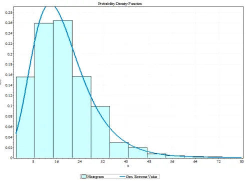
The identified distributions are listed in Table 7 with the estimated parameters for ozone concentration data set. Fig.4 showed the behavior of selected best fitted probability density function of average ozone concentration over Campo Grande. The estimated parameters were used to generate random numbers for the ozone concentration and the least squares method was used for ozone analysis.

Table 7. Estimation of parameters of identified probability distribution for the year 2016.

# Distribution Parameters

1 Exponential λ=0.0546

2 Exponential (2P) λ=0.06092 γ=1.9

3 Gamma α=3.1491 β=5.816

4 Gamma (3P) α=3.4272 β=5.5806 γ=-0.8105

5 Gen. Extreme Value k=-0.00334 σ=8.0446 µ=13.698

6 Gumbel Max σ=8.0472 µ=13.67

7 Gumbel Min σ=8.0472 µ=22.96

8 Log-Logistic α=2.8062 β=15.4

9 Log-Logistic (3P) α=4.3462 β=23.336 γ=-6.8008

10 Logistic σ=5.6902 µ=18.315

11 Lognormal σ=0.63107 µ=2.7351

12 Lognormal (3P) σ=0.37696 µ=3.2085 γ=-8.2426

13 Normal σ=10.321 µ=18.315

14 Weibull α=2.0108 β=20.506

15 Weibull (3P) α=1.6753 β=18.808 γ=1.4965

Figure 4. Graph of the histogram of best fitted probability density function for the average monthly concentration of ozone of the year 2016.

Table 8. Criteria for the quality adjustment of historical series of ozone concentration (ppb), for the winter season for the year 2016.

Chi-Squared

Exponential 0.3199 15 120.35 15 653.44 14

Exponential (2p) 0.2602 14 82.843 14 393.81 14

Gamma 0.0592 6 2.8732 4 28.591 3

Gamma (3p) 0.0508 2 2.3264 1 25.803 2

Gen. Extreme Value 0.0575 5 2.9367 5 29.736 4

Gumbel Max 0.0595 7 4.2931 8 33.123 6

Gumbal Min 0.1453 13 42.145 13 238.99 13

Log-Logistic 0.0646 8 4.8025 9 33.452 8

Log-Logistic (3p) 0.0515 4 3.7942 7 33.4 7

Logistic 0.0118 12 13.627 12 115.14 12

Lognormal 0.0471 1 2.4621 2 23.532 1

Lognormal (3p) 0.0512 3 2.7018 3 29.89 5

Normal 0.0987 11 9.7242 10 98.931 11

Weibull 0.0944 10 9.8624 11 80.259 10

(7)

Table 9. Determination of the parameters of the statistical test probability functions for winter season in the year 2016.

3 Gamma α=5.9432 β=3.0132

4 Gamma (3P) α=4.6386 β=3.4673 γ= 1.8252

6 Gumbel Max σ=5.7276 µ=14.602

7 Gumbel Min σ=5.7276 µ=21.214

10 Logistic σ=4.05 µ=17.908

11 Lognormal σ=0.42534 µ=2.7986

12 Lognormal (3P) σ=0.34214 µ=3.0125 γ=-3.6292

13 Normal σ=7.3459 µ=17.908

14 Weibull α=2.9233 β=19.958

15 Weibull (3P) α=2.1529 β=16.829 γ=3.0372

Figure 5. Graph of the histogram of ozone concentration for best fitted probability density function of winter season during the year 2016.

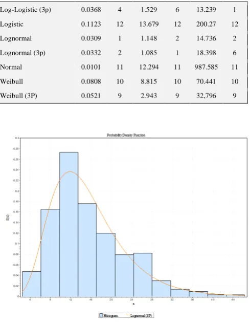
Table 10. Comparison of historical series of ozone concentration (ppb), for the spring season for the year 2016

Chi-Squared

Statistic Rank Statistic Rank Statistic Rank

Exponential 0.2929 15 103.36 15 535.99 14

Exponential (2p) 0.2384 14 68.54 14 335.52 14

Gamma 0.0418 7 1.57 7 21.577 8

Gamma (3p) 0.0385 5 1.303 4 20.477 7

Gumbel Max 0.0388 6 1.469 5 16.808 4

Gumbal Min 0.1717 13 58.084 13 248.92 13

Log-Logistic 0.0424 8 1.793 8 15.541 3

Log-Logistic (3p) 0.0368 4 1.529 6 13.239 1

Logistic 0.1123 12 13.679 12 200.27 12

Lognormal 0.0309 1 1.148 2 14.736 2

Lognormal (3p) 0.0332 2 1.085 1 18.398 6

Normal 0.0101 11 12.294 11 987.585 11

Weibull 0.0808 10 8.815 10 70.441 10

Weibull (3P) 0.0521 9 2.943 9 32,796 9

Figure 6. Graph of the histogram of ozone concentration for best fitted probability density function of spring season during the year 2016.

Table 11 Determination of the parameters of the statistical test probability functions for spring season in the year 2016.

3 Gamma α=4.5797 β=3.3792

4 Gamma (3P) α=4.0702 β=3.5711 γ= 0.94067

5 Gen. Extreme Value k=-0.02238 σ=5.6045 µ=12.114

6 Gumbel Max σ=5.6385 µ=12.221

7 Gumbel Min σ=5.6385 µ=18.73

8 Log-Logistic α=3.7051 β=13.8847

10 Logistic σ=3.987 µ=15.476

11 Lognormal σ=0.4805 µ=2.6297

12 Lognormal (3P) σ=0.3784 µ=2.860 γ=-3.2736

13 Normal σ=7.2316 µ=15.476

14 Weibull α=2.6056 β=17.258

(8)

Table 12. Criteria for the quality adjustment of historical series of ozone concentration (ppb), for the summer season for the year 2016.

Chi-Squared

Exponential 0.1805 15 51.143 15 203.73 15

Exponential (2p) 0.1274 13 21.589 13 109.27 13

Gamma 0.0555 7 4.895 7 31.863 7

Gamma (3p) 0.0485 4 3.452 5 24.564 4

Gumbel Max 0.0591 8 5.076 8 32.838 8

Gumbal Min 0.1489 14 42.117 14 153.17 14

Log-Logistic 0.0710 10 8.655 11 57.986 11

Log-Logistic (3p) 0.0523 5 4.384 6 31.581 6

Logistic 0.0944 12 12.391 12 63.343 12

Lognormal 0.0656 9 8.103 9 53.245 10

Lognormal (3p) 0.0532 6 3.194 4 26.333 5

Normal 0.0819 11 8.622 10 43.568 9

Weibull 0.0432 1 2.035 1 15.086 1

Weibull (3P) 0.0452 3 22.742 2 16.461 2

Table 13. Determination of the parameters of the statistical test probability functions for summer season in the year 2016.

2 Exponential (2P) λ=0.08698 γ=2.0667

3 Gamma α=2.9589 β=4.584

4 Gamma (3P) α= 2.0913 β=6.027 γ= 0.95965

5 Gen. Extreme Value k=-0.05615 σ=6.7483 µ=10.025

6 Gumbel Max σ=6.148 µ=10.015

7 Gumbel Min σ=6.148 µ=18.73

10 Logistic σ=4.3473 µ=13.564

11 Lognormal σ=0.6897 µ=2.4036

12 Lognormal (3P) σ=0.4129 µ=2.8897 γ=-5.9785

13 Normal σ=7.8851 µ=13.564

14 Weibull α=1.8089 β=115.166

15 Weibull (3P) α=1.4771 β=13.186 γ=1.5853

Now, probe the behaviour of ozone level on the basis of seasons.Tables 8, 9 and Fig. 5 (winter season); Tables 10, 11 and Fig. 6 (spring season); Tables12, 13 and Fig. 7 (summer season) and Tables 14, 15 and Fig. 8 (autumn season) show the summary of the komolgorov Smirnov suitability test, Anderson-Darling (AD), Chi Squared together with the estimates of the parameters of the various candidate models for the seasons of the year.

Figure 7. Graph of the histogram of ozone concentration for best fitted probability density function of summer season during the year 2016.

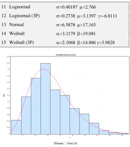
Table 14. Criteria for the quality adjustment of historical series of ozone concentration (ppb), for the autumn season for the year 2016

Chi-Squared

Exponential 0.3278 15 131.030 15 728.82 15

Exponential (2p) 0.2363 14 76.684 14 370.21 14

Gamma 0.0283 4 0.725 3 9.735 5

Gamma (3p) 0.0258 1 0.592 1 6.301 2

Gumbel Max 0.0406 8 2.406 8 21.788 9

Gumbal Min 0.1491 13 39.767 13 149.27 13

Log-Logistic 0.0490 9 2.445 9 14.227 8

Log-Logistic (3p) 0.0359 6 1.499 6 11.696 6

Logistic 0.0806 12 7.926 12 51.827 12

Lognormal 0.0301 5 1.518 7 5.836 1

Lognormal (3p) 0.0283 3 0.747 4 8.031 3

Normal 0.0784 11 5.888 10 48.588 10

Weibull 0.0667 10 6.169 11 49.879 11

Weibull (3P) 0.0389 7 0.802 5 13.064 7

Table 15. Determination of the parameters of the statistical test probability functions for autumn season in the year 2016.

2 Exponential (2P) λ=0.07754 γ=4.2667

3 Gamma α=6.7873 β=2.5287

4 Gamma (3P) 6.02 β=2.7226 γ= 0.7726

6 Gumbel Max σ=5.1365 µ=14.198

7 Gumbel Min σ=5.1365 µ=20.128

(9)

11 Lognormal σ=0.40187 µ=2.766

12 Lognormal (3P) σ=0.2738 µ=3.1397 γ=-6.8111

13 Normal σ=6.5878 µ=17.163

14 Weibull α=3.1179 β=19.081

15 Weibull (3P) α=2.1068 β=14.886 γ=3.9828

Figure 8. Graph of the histogram of ozone concentration for best fitted probability density function of autumn season during the year 2016

The selection of the best fit distribution was made based on the AD statistics and p value. A distribution with the highest p value and the lowest AD statistic is selected as the best distribution. Based on the above criteria, the best fit distributions for the datasets were identified. Thus, the best distribution for the four datasets (winter, spring, summer, autumn) is Gamma 3P; lognormal 3P; weibull and Gamma 3P.

The pdf for the best fit distributions for the four data sets is shown in Figs. 5, 6, 7 and 8. The pdf also shows the corresponding line for the mean ozone concentration of 8 hours; This clearly shows that the ozone pattern is violated during the different seasons of the year. However, the tail of the distribution is long in the case of summers.

CONCLUSIONS

A systematic evaluation procedure was applied to evaluate the performance of different probability distributions in order to identify the best fit probability distribution for the Campo Grande ozone concentration data. It was observed that the generalized extreme value distributionprovides a good fit for the whole year and the distributions: Gamma 3P; lognormal 3P; weibull and Gamma 3P for the seasons of the year: winter, spring, summer, autumn. The identification of the amount of ozone concentration data can have a wide range of applications in agriculture, engineering design and climate research.

ACKNOWLEDGMENTS

The authors would like to thank their Universities for their support.

Database statement/Availability of data

The meteorological database is public domain and is available at: Center for Monitoring Weather, Climate and Water Resources of Mato Grosso do Sul (Cemtec / MS), an agency linked to the State Secretariat of Environment, Economic Development , Production and Family

Agriculture (Semagro), http://www.cemtec.ms.gov.br/laudos-meteorologicos/.

The ozone pollutant database belongs to the physics institute of the federal university of mato grosso do sul and may be requested from Prof Dr Amaury de Souza, email [email protected]

REFERENCES

1_{Souza, A., Ozonur, D., Statistical Behavior of O}

3, OX, NO,

NO2, and NOx in Urban Environment, Ozone: Sci. Eng., 2019, 1-13. DOI: 10.1080/01919512.2019.1602468

2_{Catalunha, M., J., Sediyama, G. C. , Leal, B. G. , Soares,. C. P. B.,}

Ribeiro, A., Aplicação de cinco funções densidade de probabilidade a séries de precipitação pluvial no Estado de Minas Gerais, Rev. Brasil. Agrometeorol., 2002, 10(1), 153-162.

3_{Souza, A., et al. "Probability distributions assessment for}

modeling gas concentration in Campo Grande, MS, Brazil." European Chemical Bulletin 6.12 (2018): 569-578.DOI: 10.17628/ecb.2017.6.569-578

4_{Souza, A., Olaofe, Z., Kodicherla, S. P. K., Ikefuti, P., Nobrega,}

L., Sabbah, I., Modeling of the Function of Distribution of the Ozone Concentration of Surface to Urban Areas, Eur. Chem. Bull., 2018, 7(3), 98-105. DOI: 10.17628/ecb.2018.7.98-105.

5_{Jan, B., Zai, M. A. K. Y., Abbas, S., Hussain, S., Ali, M., Ansari,}

M. R. K., Study of probabilistic modeling of stratospheric ozone fluctuations over Pakistan and China regions, J. Atm. Solar-Terrestrial Phys., 2014, 109, 43-47. doi.org/10.1016/j.jastp.2013.12.022

6_{Júnior, J. A.,}_{Gomes, N. M., Mello, C. R., Silva, A. M.,}

Precipitação provável para a região de Madre de Deus, Alto Rio Grande: modelos de probabilidades e valores característicos." Ciênc. Agrotecnol., 2007, 31(3), 842-850. doi.org/10.1590/S1413-70542007000300034

7_{Lyra, G. B.,}_{Garcia, B. I. L., Piedade, S. M. S., Sediyama, G.}

C. and Sentelhas, P. C., Regiões homogêneas e funções de distribuição de probabilidade da precipitação pluvial no Estado de Táchira, Venezuela, Pesquisa Agropecuária Brasil., 2006, 41(2), 205-215.

8_{Ferreira, F. F. Estatística Básica. 1. ed. Lavras: Editora UFLA,}

2005, 664 p.

9_{Sharma, M. A. and Jai, B. S., Use of probability distribution in}

rainfall analysis, New York Sci. J., 2010, 3(9), 40-49.

10_{Laha, R. G., Chakravarti, J. R., Handbook Methods of Applied}

(10)

11_{Stephens, M. A.“Goodnessof Fit with Special Reference to Tests}

for Exponentially”, Tech. Rep. No. 262, Department of Statistics, Stanford, CA, 1977.

12Souza, A., Kovač_{-Adnric, E., Matasovic, B., Markovic, B.,}

Assessment of Ozone Variations and Meteorological Influences in West Center of Brazil, from 2004 to 2010. Water, Air and Soil Pollut., 2016, 227, 313. DOI: 10.1007/s11270-016-3002-0

13_{Ministério do Meio Ambiente , MMA. Conselho Nacional de}

Meio Ambiente – CONAMA. Resolução no 003 de 28 de junho de 1990, dispõe sobre padrões da qualidade do ar. Disponível

http://www.mma.gov.br/port/conama/legiabre.cfm?codlegi=1 00

14_{de Souza, A., Guo, Y., Pavão, H. G. and Fernandes, W. A.}

Effects of Air Pollutionon Disease Respiratory: Structures Lag., Health, 2014, 6, 1333-1339. http://dx.doi.org/10.4236/health.2014.612163

15_{Kassem, K. O., Statistical analysis of hourly surface ozone}

concentrations in Cairo and Aswan/Egypt. World Environ., 2014, 4(3), 143–150. doi:10.5923/j.env.20140403.05