Vol 2013

(1)

ISSN 2307-7743 http://scienceasia.asia

_______________

*_{Corresponding author}

2010 Mathematics Subject Classification: 41A50

Key words and phrases: Markov Inequality, Probability Distributions, Continuous random variable, Bound, Measure Space and Sharp

ON INEQUALITY TO GENERATE SOME STATISTICAL DISTRIBUTIONS

A. F. OGUNTOLU* 1_{, U. Y. ABUBAKAR}1_{, A. ISAH}1_{, L. A. NAFIU}1_{AND K. RAUF}2

ABSTRACT. In this work, we established Markov inequality via Binomial, Poisson and Geometric Distribution. Results obtained were used to obtain probability bound for some random variables. Our results are in

agreement with the existing works.

1. INTRODUCTION

Markov inequality states that:

For any nonnegative random variable X and a > 0, we have the following inequality

This is equivalent to the following inequality in measure theory:

Where (X, Σ, μ) is a measure space, ƒ is a measurable extended real-valued function,

and .

This definition is sometimes referred to as Chebyshev’s or Bienayme’s inequality in analysis because it appearsed without prove in, at least, the work of Pafnuty Chebyshev who happened to be Markov’s teacher (Stein and Shakarchi).

Markov’s inequality (Markov (1884)) is useful in providing an upper bound for the probability of a random variable with a non negative function which is greater than or equal to some positive constant. It also relate probabilities to expectations.

In particular, it is applicable in proving Chebyshev’s inequality (Chebyshev (1874)) and in showing that for a nonnegative random variable, the mean and a median are such

that .

(2)

see Salo-Coste (1997), Ross (1976), Steliga and Szynal (2010), Feller (1966), Papoulis (1991), Clarkson et.al. (2009), DasGupta (2000), McWilliams (1990), Pitman (1993), Pfeiffer and Schum (1973).

2.0 Materials and Methods

This section consider the prove of Markov inequalityy and its application to some properties of some distributions.

2.1 The prove of Markov Inequality

THEOREM: Let X be a random variable and assume that its range is a subset of non-negative real numbers. Assume that E[X] exists. Furthermore let A be some

positive constant, then,

A X E A

X ) [ ]

Pr(  

Proof (Discrete): Let X be a discrete random variable. The proof is almost trivial; we

only have to recall the notion of the mean of a random variable. It is



_



i

i X Z

Z X

E[ ] Pr( )

Where Zi is the sequence of the range of X .The right hand side contains just non-negative elements, thus we decrease this sum if we restrict it to those Z_i  A

_

  

 

 

i z A z A z A

i i

i i i

z X A

z X A Z

X Z

Z X Z

X

E[ ] *Pr( ) *Pr( ) *Pr( ) * Pr( )

We can rewrite

_



 A

z

i

z

X )

Pr( as Pr( X  A),

) Pr(

* ]

[X A X A

E   and

A X E A

X ) [ ]

Pr(  

(3)



 

 

t x

dx t

X ) 

Pr(

Let U  x then du  dx and V  x then dv  x. Hence,



  

 _

 

t x t

x

dx x x

t

X )  | 

Pr(

| [ ]

x t

x   E X t

  

[ ]

x

t  E X t

  

[ ] [ ]

x

t  E X E X t

   

t X E t

X ) [ ]

Pr(  



2.2 Properties of Binomial Distribution

The Binomial Distribution is given by

x n x

n

x

P P

X   

    

 .(1 )

] Pr[

While the Cumulative Probability is







        

n

x

x n x

n

x

P P

X

0

) 1 .( ]

0 Pr[

0

!

.(1 ) ( ) ! !

n

x n x

x

n

P P

n x X





 





1

(1 ) (1 )

! ...

! 0 ! ( 1) !(1) ! 0 ! !

n n n

P P P P

n

n n n



   

 _    _



 

By Binomial expansion, we have



n n n n



P P nP

P nP P

n n

X   (1 )  (1 )  ...   (1 ) !

! ] 0

Pr[ 1 1

1 1 ) 1 ( ] 0

Pr[ X   P   P n  n 







 

 

n

x

x n x

P P x x x n

n x X

E

0

) 1 ( )! 1 ( )! (

! ! ]

(4)

0

!

(1 ) ( ) !( 1) !

n

x n x

x

n

P P

n x x

     



1 0

( 1) !

. (1 ) ( ) !( 1) !

n

x n x

x

n n

P P P

n x x

       



1 0

( 1) !

. (1 ) ( ) !( 1) !

n

x n x

x

n

n P P P

n x x

       



Mean=E[X] nP(1)  nP



     n x x n x P P x x n n x X E 0 2 2 ) 1 ( ! )! ( ! ] [ 0 ! (1 ) ( ) !( 1) !

n

x n x

x

x n

P P

n x x

     



0 0

( 1) ! !

(1 ) (1 )

( 1) !( 1) ( 2 ) ! ( ) !( 1) !

n n

x n x x n x

x x

x n n

P P P P

n x x n x x

             



2 1 0 0

( 1) ( 2 ) ! ( 1) !

. . (1 ) . (1 )

( ) !( 2 ) ! ( ) !( 1) !

n n

x n x x n x

x x

n n n n n

P P P P P P P

n x x n x x

                



2 2 1

0 0

( 2 ) ! ( ) !

( 1) (1 ) (1 )

( ) !( 2 ) ! ( ) !( 1) !

n n

x n x x n x

x x

x n x

n n P P P n P P P

n x x n x x

                



2

( 1) (1) (1)

n n P n P

  

2 2

[ ] ( 1)

E X n n P n P

   

Variance ( 2 2 2

]) [ ( ] [ ] [

)Var x  E X  E X

 ) 2 2 2 ) ( ) 1

(n P nP nP

n   

 

2 2 2 2 2

n P n P n P n P

   

We have the variance as: Variance

 

 2  nP(1 P)

2.3 Prove of Markov Inequality from Binomial distribution

_

           n x x n x n x P P a X 0 ) 1 .( . ] Pr[ 0

. .(1 )

n n

x n x

x x x P P x      _{ }   



0 1

. . .(1 )

n n

x n x

x x

x P P

x      _{ }   



1 (n P)

x

(5)

But,

a x a

x   1  1 . Hence,

a nP nP a a

X  ] 1 ( ) 

Pr[

2.4 Poisson Distribution

The Poisson distribution is given by

! ] Pr[ x X x      Cummulative Probability

_



_

       

0 ! 0 !

] 0 Pr[ x x x x x x

X   

   1     

_



_

       

0 ! 0( 1)!

. ] [ x x x x x x x X E   _   

_



_

              0 0 1 1 . )! 1 ( )! 1 ( x x x x x x                  E[X] Mean







        0 0 2 2 )! 1 ( . ! . ] [ x x x x x x x x X E   _    0 0

( 1) .

( 1) ! ( 1) !

x x x x x x x               



1 0 0 .

( 2 ) ! ( 1) !

x x

x x x x

               



2 1 2 0 0 .

( 2 ) ! ( 1) !

x x

x x x x

                 



2     2 2 2 ]) [ ( ] [ ] [ )

( Var X E X E X

Variance    

2 2

[ ]

V a r X    

    

Hence, we have the variance as:

2       _    . ]

(6)

2.5 The prove of Markov’s Inequality from Poisson distribution

_



_

        a

x x a

x x x x x x a X ! ! ] Pr[   _   

1 . 1

! ( 1) !

x x

x a x a

x

x x x x

            



1

( 1) !

x x a x x         



1

0 ( 1) !

x

x x x

          



If a X a

X   1  1

Hence,

a a

X  ] 

Pr[

2.6 Geometric Distribution

The Geometric Distribution is given by

x

P P

X ] (1 )

Pr[  

The Cummulative Probability is



       0 0 ) 1 ( ) 1 ( x x x x P P P P

Let a 1 P  a 1 P



      0 0 ) 1 ( x x x x a P P P



              0 1 1 1 ) 1 ( ) 1 ( 1 1 1 1 x x x x x a a P a a a a a



                    0 1 1 1 1 0 ] ) 1 ( 1 [ ) 1 ( ) 1 ( ) 1 ( ] Pr[ x x x x x x x P a a P a P a P X

As x1  where 0  P 1, (1 P)  0



     0 1 ) 0 1 ( ] Pr[ x X

(7)



      0 0 ) 1 ( . ] Pr[ . x x x P P x X x

Let a 1 P



     0 0 . ] Pr[ . x x x a x P X x







                    0 2 1 2 1 ) 1 ( ... 1 ) 1 ( 1 1 ] Pr[ . x x x x a a a a a a a a a a P X x







             0 2 1 1 2 ) 1 ( .... ) 1 ( ) 1 ( 1 ] Pr[ . x x x x x a a a a a a a a P X x

Since P 1a

)] 1 ( ) 1 ( .... ) 1 ( ) 1 [( ]

[X a a a a 1 a 2 a2 a 1 a

E   x   x   x   x 

1

x

a

a x a

a

  

 _ _



 

As x 0 within 0  P 1 for a 1 P

x x

P

a  (1 )  0 since 0  (1 P)1

a a a a a a X E                     1 1 1 0 1 0 1 ] [ 1 1

1 (1 )

P P P P       Mean= P P X

E[ ] 1

The Variance is,



   0 2 2 . . ] [ x x a x P X

E where a 1 P

_

   0 2 2 . ] [ x x a x P X E 2

2 2 1 2 2 2 1 2 2 1 1

[ (1 0 ) ( 2 1 ) ...[ ( 1) ( 2 ) ]

1 1 1

x x

x

a a a

P a a x x a

a a a

            _ _  _ _    _ _          ] ) ) 1 (

(x2  x 2 ax

2 2 2 2 2 2 2 2 2 1

[ (1 0 ) ( 2 1 ) . . . . [ ( 1 ) ( 2 ) ]x [ ( 1 ) ]x

a a x x a  x x a 

            

[(12  02) (22 12)... [(x1)2 (x 2)2][x2 (x 1)2]ax]

0 0 0

( 2 x x) [ x ( 2 1) ]

x x x

a x a a a x

  

  

 

 _    _

(8)

But

_

             0 1 1 1 x x x x xa a a a a

xa And



    0 2 ) 1 2 ( x x x 2 1 1 2 2 . 1 1 1 1 1 2 ] [                              x x x a x a a xa a a a a a X E

As x   , ax  0

                                     0 1 1 0 1 1 1 2 ] [ 2 a a a a a X E

2 2 2

2 2 (1 )

(1 ) 1 (1 ) (1 )

a a a a a a a

a a a a

  

   

   

2

(1 P) (1 P)

P

  



We have the variance as:

Variance 2 2 2

]) [ ( ] [ ]

[X E X E X

Var  

  2 2 2 2

2 (1 ) (1 ) (1 )

P P P P P      

 (1 ₂P)

P

 

2.7 Prove of Markov’s Inequality from Geometric distribution

_

     a x x P P a

X ] (1 )

Pr[

(1 )x

x a x P P x   





1 . (1 )x 1 [ ] 1 1

x a

P

x P P E X

x x x P

         _ _  



But a X a

X   1  1

a X E a

X ] [ ]

Pr[   1 P

a P

(9)

3. Tightness of Markov’s Inequality

Markov Inequality provides a weak bound because the amount of information provided to it is limited. All the information provided to it were that the variable is non-negative and that the expected value is known and finite. Now, we will show that it is indeed tight -that is Markov Inequality is already doing as much as it can. Consider a random variable X such

that

  

  

 



else 0

k 1 prob. with

k

X

We can estimate its expected value as:

1 0 * 1 *

1 ]

[    

k k k k X E

   

k k X X

kE

X [ ] Pr 1

Pr    

This implies that the bound is tight because the value of the random variable is exactly k or otherwise zero.

4. Results

We use Markov inequality to analyze Binomial distribution, Poisson distribution and

Geometric distribution given that the initial probability distribution is

a

P  1 where a _{is a}

positive natural number .

(10)

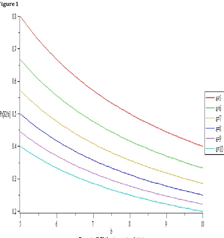
Markov Inequality from binomial distribution

b X E b

X ] [ ]

Pr[   n p

b

 . But,

a P  1 and

b a

n b X

. ] Pr[  

We consider the equation for the graph as:

b a

n b X

. ] Pr[  

(11)

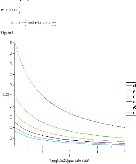
Markov Inequality from Poisson distribution

b b

X  ] 

Pr[

But

a

1



 and  

b a b X

. 1 Pr  

(12)

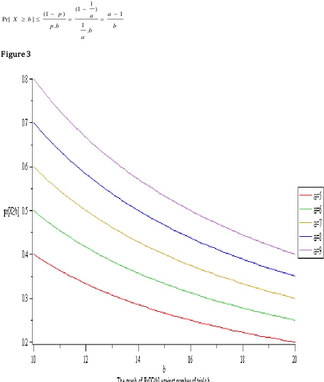
Markov Inequality from Geometric distribution

b a

a

b p

p b

X 1

. 1

) 1 1 (

. ) 1 ( ]

Pr[  

    

(13)

4 Discussions

In Figure 1, we observe that with increase in the value of 'a' the probability steadily

reduces. Also, it can be observed that as the number of trials increases, the probability of the event will considerably reduce.

In Figure 2, we observe that with increase in the value of 'a' ,the probability steadily

In Figure 3, we observe that with increase in the value of'a', the probability steadily

5 Conclusions

The use of Markov inequality to analyze the Binomial distribution is inadequate because it gives unrealistic inequality variation, thus making it difficult to properly establish a realistic bound for the probability of higher value, hence a new approach is required to establish a more realistic bound.

The use of Markov inequality to analyze the Poisson distribution is adequate because it gives a suitable inequality variation thereby enhancing a realistic bound for the probability distribution.

The use of Markov inequality to analyze the geometric distribution is inadequate because it gives realistic values for higher values of 'b' with lower values of 'a' but becomes

(14)

REFERENCES

[1] Salo-Coste, L (1997). Lectures on finite Markov chains. Lectures on probability theory and statistics (Saint-Flour Summer School, 1996), 301-413, Lecture Notes in Math., 1665, Springer, Berlin.

[2] Ross, Sheldon (1976) A First Course in Probability, Macmillan Publishing Company, New York, New York, 1976.

[3] Steliga, K and Szynal, D. (2010) "On Markov-type Inequality", International Journal of Pure and Applied Mathematics, 58(2) 137-152.

[4] Chebyshev, P. (1874). Sur les valeurs limites des integrales, J Math Pure Appl 19: 157-160.

[5] Feller, W. (1966) An introduction to probability theory and its applications. Vol II, 2nd ed. Wiley, New York pp155.

[6] Markov, A. (1884). On certain applications of algebraic continued fractions, Ph.D. thesis, St Petersburg. [7] Papoulis, A. (1991), Probability, Random Variables, and Stochastic Processes, 3rd ed. McGraw-Hill. ISBN

0-07-100870-5. pp. 113-114.

[8] Stein, E.M. and Shakarchi, R. (2005) "Real Analysis, Measure Theory, Integration, & Hilbert Spaces", vol. 3, 1st ed., 2005, p.91.

[9] Clarkson E, Denny JL, Shepp L (2009) ROC and the bounds on tail probabilities via theorems of Dubins and F. Riesz. Ann Appl Prob 19 (1) 467-476 DOI: 10.1214/08-AAP536.

[10] DasGupta A. (2000). Best constants in Chebyshev inequalities with various applications. Metrika, 51: 185-200.

[11] McWilliams T.P. (1990). A distribution-free test for symmetry based on a runs statistic. J Am Stat Assoc 85 (412)1130-1133.

[12] Pitman, Jim. Probability (1993 edition). Springer Publishers. pp. 372.

[13] Pfeiffer, P. E. and Schum D. A. (1973). Introduction to Applied Probability. New York: Academic Press, 1973.

1_{DEPARTMENT OF MATHEMATICS AND STATISTICS, FEDERAL UNIVERSITY OF TECHNOLOGY, MINNA,}

NIGERIA