COLUMN TESSELLATIONS

COLUMN TESSELLATIONS

N

L

N

V

W

R

C

1_{Friedrich-Schiller-Universit¨at Jena, Institut f¨ur Stochastik, Germany;}2_{Ernst-Abbe-Hochschule Jena,}

Fachbereich Grundlagenwissenschaften, Germany;3School of Mathematics and Statistics, University of Sydney, Australia

e-mail: [email protected],[email protected], [email protected] (Received February 3, 2015; revised May 19, 2015; accepted May 26, 2015)

ABSTRACT

A new class of non facet-to-facet random tessellations in three-dimensional space is introduced – the so-called column tessellations. The spatial construction is based on a stationary planar tessellation; each cell of the spatial tessellation is a prism whose base facet is congruent to a cell of the planar tessellation. Thus intensities and various mean values of the spatial tessellation can be calculated from suitably chosen parameters of the planar tessellation.

Keywords: combinatorial topology, random tessellations, stochastic geometry.

THE CONTEXT FOR OUR NEW

MODEL

Random tessellations are classical structures considered by stochastic geometers. Two standard models are the Poisson hyperplane and Poisson Voronoi tessellations (Schneider and Weil, 2008; Chiu et al., 2013). In the planar case these tessellations are side-to-side, that is, each side of a polygonal tessellation cell coincides with a side of a neighbouring cell. In their three dimensional versions they are facet-to-facet, meaning that each facet of a polyhedral cell coincides with a facet of a neighbouring cell.

In recent years there has been a growing interest in tessellation models that do not have the stated coincidence for all sides or facets. A first systematic study of the effects when a three-dimensional tessellation is not facet-to-facet is given in Weiss and Cowan (2011). A recent study presented in Cowan and Th¨ale (2014) looks in depth at the planar case, building on results from the 1970s when non side-to-side tessellations first attracted attention.

Tessellations of that kind arise for example by cell division. Among these models, theiteration stable or STIT tessellation is of particular interest because of the number of analytically available results (Nagel and Weiss, 2005; Mecke et al., 2008; Th¨ale et al., 2012; Cowan, 2013; Th¨ale and Weiss, 2013, and the references therein). It serves as a reference model for geological crack and fissure structures (Mosser and Matth¨ai, 2014) and might have application in the process of biological cell division. The development of new model classes is important for further applications to random structures in materials science, geology and biology – and the current paper contributes to that aim.

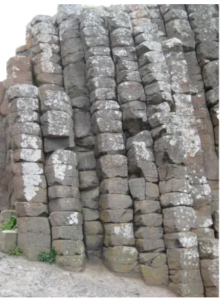
We consider a new class of non facet-to-facet spatial tessellations, whose construction is based on a stationary planar tessellation Y0 having convex polygonal cells. From each polygonal cell z of Y0 we form an infinite column perpendicular to the plane E in which Y0 lies. Any cross-section of the column parallel to E is congruent to z. To create a spatial tessellation, each infinite column is intersected by many such cross-sections, thereby dividing the column into cells. The spatial cells which arise are prisms and their polygonal base facets (located at the cross-sections) are translations (in the third dimension orthogonal to E) of the cells of Y0. The resulting three-dimensional tessellation Y is called a column tessellation. Column tessellations could be useful to describe crack structures in geology, as for example in the Giant’s Causeway of Northern Ireland (Figs. 1 and 2).

If the locations of cross-sections were identical in all columns, the column tessellationY reduces to the stratum model of (Mecke, 1984) and is facet-to-facet if and only if Y0 is side-to-side. So, in order to be innovative, we shall be introducing mechanisms such that no section which divides a column is coplanar with a section of a neighbouring column. This implies that cells in neighbouring columns will not have a common facet. As a consequence, the tessellations we shall study in this paper are never facet-to-facet.

parameters of the planar tessellation are necessary to calculate characteristics of the spatial tessellation. This is interesting, for example, when only a planar section through a spatial column tessellation can be observed.

Fig. 1. Basalt columns, approximately 6−8 metres high above ground level, divided by ‘cross-sectional plates’ at approximately 30 cm spacing. Photo taken by one of the authors. There are many formations like this one (at the Giant’s Causeway, Northern Ireland) around the world.

The paper is organized as follows. To describe in detail the complicated geometry for tessellations which are not facet-to-facet, we use the system of notation given in (Weiss and Cowan, 2011). The next section gives a short introduction to this notation for planar and spatial tessellations. In Section “Column tessellations”, the general construction of a column tessellation is explained, special notation is defined and basic properties are considered. Section “Formulae for the features of column tessellations” shows that intensities and various mean values of a spatial column tessellation can be determined by suitably chosen parameters of the planar tessellation. Later in that section, formulae for metric mean values of the column tessellation are also deduced. Three examples conclude the paper.

To aid comprehension throughout the paper, we often consider the special case where the cross-sectional plates in a column have a constant separation

of 1 unit. This generates a column tessellation where all the cells have height 1. We illustrate the notation and our results using this special case.

Fig. 2. Viewed from above, examples of pentagonal and heptagonal basalt columns at the Giant’s Causeway.

BASIC DEFINITIONS AND THE

NOTATION USED

The geometric elements: In this paper we describe stationary convex-celled random tessellations inR2andR3in general terms. We use the structure and

system of notation given in Weiss and Cowan (2011), where convexity of cells was also assumed. Convexity implies that the cells in the R2 case are convex

polygons and, in theR3case, convex polyhedra.

polygons imbedded in anR3-tessellation. For example,

cell-facets in a tessellation ofR3 are polygons; so we

can speak offacet-sidesandfacet-corners.

For a spatial tessellation, we deal with four kinds ofprimitive elements: these are calledvertices,edges, platesandcells. They are defined as follows.

A tessellation of R3 is a locally-finite collection

of compact convex cells which cover the three-dimensional space and overlap only on their boundaries. The union of the cell boundaries is called the tessellationframe. A subset of the frame, the union of all the cell-ridges, is called the tessellation net. Each cell has apices, ridges and facets which lie on the frame, the first two lying in the net. The union of all apices is a collection of points inR3 called the

verticesof the tessellation. Those line-segments which are contained in the net, have a vertex at each end and no vertices in their relative interior are called edges of the tessellation. Those convex polygons which are contained in the frame, whose boundary is contained in the net and whose relative interior is disjoint from the net are calledplates.

So we see that vertices, edges, plates and cells are elements of the tessellation, whilst apex, ridge and facet are names for elements of a polyhedral cell. Vertices, edges, plates and cells are primitive in the sense that they cannot have any other elements in their relative interior.

Classes of elements and their inter-relation: The corresponding classes of these primitives are denoted byV,E,PandZ. An object belonging to a classXis often referred to as “anX-type object” or “an object of typeX”.

For a random tessellation the intensity of objects of class X is denoted by λX. It is the mean number of centroids of X-type objects per unit volume. By definition, thecentroidof a nonempty compact subset C of Rd is the centre of the (uniquely determined)

smallest ball containingC(Schneider and Weil, 2008, Section 4.1). It is assumed henceforth that 0<λX<∞; this is the case for all examples considered. Recall that an objectxofX is said to beadjacentto an object y

of Y if either x⊆y or y⊆x. Let µXY be the mean number ofY-type objects adjacent to the typical object of X. Formally the typical object of class X can be introduced by means of Palm distributions for which we refer to Schneider and Weil (2008) and Chiuet al. (2013). Intuitively it can be considered as a uniformly selected object from X independently of its size and shape. For an element x∈ X the number of Y-type objects adjacent tox is denoted by mY(x). Formally, we write µXY := EX[mY(x)], where EX denotes an

expectation for the typical object of typeXwith respect to the Palm distribution.

Because of combinatorial and topological relations within any particular spatial tessellation the twelve adjacency mean values µXY, for X,Y ∈ {V,E,P,Z}

andX6=Y, can be expressed for a random tessellation as functions of just three parameters; they have cyclic subscripts.

µVE – the mean number of edges emanating from the typical vertex,

µEP – the mean number of plates emanating from the typical edge and

µPV – the mean number of vertices on the boundary of the typical plate.

See Weiss and Cowan (2011) or also Radecke (1980) and Mecke (1984) where another notation is used. Note that all twelve adjacencies are invariant under topological transformations of R3, defined in

Gr¨unbaum and Shephard (1987, page 166). So we call

µVE,µEPandµPVthetopological parameters.

In the facet-to-facet case, the j-dimensional faces of anX-type object are primitive elements. In contrast, for non facet-to-facet tessellations we must carefully distinguish between the primitive elements and the j-faces of polytopes. For example a cell can have vertices on its boundary which are not 0-faces of that polytope. A 1-face (ridge) of a cell can have vertices in its relative interior, this being impossible for edges. A 2-face (facet) of a cell may not be a plate. Hence we use the notation Xj for the class of all j-faces of

X-type polytopes, j<dim(X-object). For instanceP1 is the class of the 1-dimensional faces of all plates, called the plate-sides. We emphasize that some of these classes aremultisetsbecause of the multiplicities of the elements. For example if k cells have a 0-face located at a vertex v, then the class Z0 has k elements positioned on v; note that here k ≤mZ(v). Furthermore, we definenj(x)as the number of j-faces of a particular objectx∈Xandνj(X):=EX[nj(x)]is

the mean number of j-faces of the typical X-object. For example it is

ν0(P) – the mean number of 0-faces of the

typical plate,

ν1(Z) – the mean number of 1-faces (ridges)

of the typical cell.

Sometimes we use X[·] for a subset of the class X, where the term in the brackets is a suitably chosen symbol describing the property of the subclass. For example, the subclasses of horizontal and vertical edges are denoted byE[hor]andE[vert]respectively.

element can have interior structure. To quantify the effects of this phenomenon four additional parameters for a random tessellation were introduced in Weiss and Cowan (2011). They are calledinterior parametersand defined as follows:

ξ – the proportion of edges whose interiors

are contained in the interior of some cell-facet,

κ – the proportion of vertices in the

tessellation contained in the interior of some cell-facet,

ψ – the mean number of ridge-interiors

adjacent to the typical vertex,

τ – the mean number of plate-side-interiors

adjacent to the typical vertex.

Note that the interior parameters can be written using the adjacency notation as

ξ=µ_EZ◦ ◦₂, κ=µ_VZ◦₂, ψ=µ_VZ◦₁ and τ=µ_VP◦₁,

using

◦

Xfor the class of relative interiors of members of X. We call an edge whose interior is contained in the interior of a cell-facet a π-edge and a vertex in

the interior of a cell-facet a hemi-vertex (Weiss and Cowan, 2011).

Naturally all four interior parameters are zero in the facet-to-facet case. In Cowan and Weiss (2015) it is shown that a random spatial tessellation is facet-to-facet if and only ifξ =0. Some further notation will

be given later.

The planar tessellation: The initial template for the construction of a column tessellation is a stationary planar tessellation Y0 in a fixed plane E which, without loss of generality, is assumed horizontal. The classes of planar primitive elements of Y0 are V0

(vertices), E0 (edges) and Z0 (cells); analogously to the spatial case these entities are defined for planar tessellations (Cowan and Th¨ale, 2014). For example, an edge of a planar tessellation is a line segment which is contained in the frame, has a vertex on each end and no vertices in its relative interior. All the intensities λ_X0 and the adjacency mean values µ_XY0 , X,Y ∈ {V0,E0,Z0} are marked with an apostrophe. The subscripts are always written without apostrophes. A planar tessellation which is not side-to-side has vertices located in the interior of cell-sides. We call them π-vertices, because one angle created by the

emanating edges is equal toπ. Theinterior parameter of a random planar tessellation is

φ – the proportion ofπ-vertices in the

tessellation,φ=µ0

V

◦

Z1

.

Two cells of a planar tessellation are called

neighbours if their intersection is an edge of the tessellation.

COLUMN TESSELLATIONS

Construction: Based on the planar tessellation Y0 _{in the horizontal planeE we construct the spatial}

column tessellationY in the following way:

For each cell z of Y0, we consider an infinite cylindrical column based on this cell and perpendicular toE. Further we markz’s centroid with a real-valued positive ρz. Here, conditional upon Y0, ρz is a non-random function of some aspects of Y0 viewed from

z, for example, the size, shape or environment of the cellz. (Unconditionally, ρzinherits some randomness fromY0.) Such a mark is created for all cells inY0. Now, for each planar cell z, we construct on the line going through the cell-centroid ofzperpendicular toE – we call this the cell-axis – a stationary and simple point process with intensity ρz. This point process

may be dependent on the cell-axis point processes forneighbouring columns(the columns based on two neighbouring cells ofY0), but we require the following property.

Property 3.1. The simple superposition property: We require that the superposition of the cell-axis point processes of two neighbouring columns be a simplepoint process, that is, a point process without multiplicities.

To create the spatial tessellation, the column based on zis intersected by horizontal cross-sections located at each of the random points of that column’s point process. The resulting tessellation Y is called a column tessellation. Note that the cell-axes do not belong to the column tessellation. Because the horizontal cross-sections are actually plates of Y, and there are no other plates in the tessellation that are horizontal, we shall often refer to them as the horizontal plates.

Any cell ofY is a right prism, where its base facet is a vertical translation of a cell of Y0. Because of Property 3.1, there is no coplanarity of cross-sectional plates that appear in neighbouring columns, and so the cells in neighbouring columns cannot have a common facet. So a column tessellation is not facet-to-facet. The intersection of a column tessellationY with any plane parallel toE is a vertical translation ofY0.

Constant cell heights: Letζk, k=0,±1,±2, ...,

be the random distances of the horizontal plates from E. A very simple case arises when ζ0 is uniformly

implies, of course, thatρz=1, a constant for all cellsz of Y0. Also the positions of the horizontal plates in a column are stationary and completely independent of such plates in the neighbouring columns, as no information has been drawn fromY0.

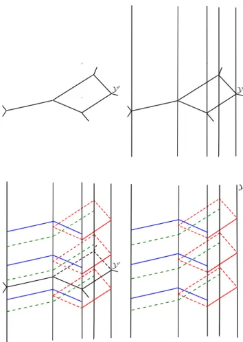
Fig. 3.Column tessellationY with constant height1. Here the four steps building up a column tessellation are shown: Starting with the planar tessellation Y0, next the columns are given by the cells ofY0. Then the columns with their cuts are shown, whereas in the last figureY0is removed, it is no part ofY.

Any cell of the column tessellation Y that has arisen is a right prism with height 1. For short, we call it acolumn tessellation with height 1. An illustration is given in Fig. 3. On the top on the left the planar tessellationY0 is shown and the columns formed by the cells of Y0 on the right. On the bottom left we see the columns with the cuts generated by the parallel horizontal plates, using three different colors for three columns. Down the right we strikeY0off because it is not a part of the column tessellationY.

More notation: We need further notation for planar tessellations. Some is based on a relationship between cells and lower dimensional objects of the planar tessellation - an ownership relation. We

describe the ownership relation using a function b (belonging to) defined as follows. Ifzj is a j-face of

a cell z, j=0,1, then it belongs to that cell and we writez=b(zj) to identify the owner. In other words, cellzis the owner of any j-facezjsuch thatz=b(zj).

It is obvious thatz is the owner of nj(z) j-faces and

that anyzj ∈Z0jhas its unique owner. (Remember that

Z0j is a multiset.) Furthermore we are interested in the

vertices of a cell which are not corners (0-faces) of that cell. It is obvious that those vertices areπ-vertices. We

say that z is the owner of such a π-vertex which is

not a 0-face of z. We use for this special belonging to function the symbol bπ. Thus any π-vertex v[π]

belongs to a unique owner-cellz=bπ(v[π])and a cell

zownsmV(z)−n0(z)π-vertices. So our belonging to

functionbhas domainZ00∪Z10and rangeZ0, whereas functionbπ has domainV0[π]and rangeZ0.

Later we will investigate the dependency of the vertex intensity of a column tessellation on both the planar tessellation and the given marks ρz. It is easy to see that all vertices of Y are located on vertical lines through the vertices of Y0. Also the intensity of the vertices on such a vertex line depends on the ρ

-intensity of all the planar cells adjacent to the planar vertex which creates this vertex line. To describe those relations between Y, Y0 and the cell marks ρz we define further entities for the planar tessellationY0 as follows.

– Whenxis adjacent toz∈Z0,

αx:=

∑

{z:z⊃x} ρz,

where we mostly consider the cases x=v∈V0,

x=e∈E0andx=v[π]∈V0[π].

– Whenz∈Z0 ownsz0∈Z00 orv[π]∈V0[π],

βz0 :=ρb(z0) and

βv[π]:=ρbπ(v[π])

wherez0is a 0-face of the cellb(z0)andv[π]is a π-vertex and no 0-face of the cellbπ(v[π]).

Furthermore,

– if`0(e) is the length of the edgeeanda0(z)is the area of the cellz,

γv:=m0E(v)αv (number-weighted),

γe:=`0(e)αe (length-weighted),

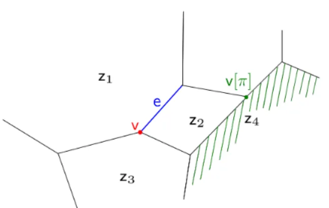
Fig. 4. An example of adjacency and ownership relations in the planar tessellationY0.

Fig. 4 illustrates an example that shows our notation – and also the differences between the ownership and adjacency relations. The vertex v is adjacent to the cellsz1,z2andz3, the edgeeis adjacent

to the cellsz1 andz2, hence αv=ρz1+ρz2+ρz3 and

αe=ρz1+ρz2.For the ownership relation, it is easy to see that for theπ-vertexv[π]we haveβv[π] =ρz4, because z4 =bπ(v[π]). Besides, v is a 0-face of the

cells z1, z2 and z3, then the classZ00 has 3 elements located onvdenoted byz01,z02 andz03(not shown in the figure) with owner-cellsz1,z2andz3, respectively. Henceβz01=ρb(z01)=ρz1,βz02=ρz2 andβz03=ρz3.

Later we will see that the last two items of the new notation, γe and γz, are necessary for the studies of the metrical properties whereas all others are used for results concerning topological and interior parameters. All these α-, β-, γ-quantities can be understood as

marks of elements of the planar tessellation. Each of these marks leads to mark distributions. The corresponding means in the random context are as follows:

– ρ¯Z=E0Z(ρz) – the meanρ-intensityof the typical cell;

– α¯X =E0_X(αx) – the mean total ρ-intensity of

all cells adjacent to the typical X-object, X ∈ {V0,V0[π],E0};

– β¯Z0 =E

0

Z0(βz0) and ¯βV[π] =E0_V[π](βv[π]) – the

meanρ-intensity of the owner cell of the typical 0-face or the typicalπ-vertex, respectively;

– γ¯X=E0X(γx) – the meantotal weightedρ-intensity of all cells adjacent to the typical X-object, X∈ {V0,E0,Z0}.

Remark 3.2. Using mean value identities for the primitive tessellation elements, given in (Møller, 1989), and some generalisations, most of the above

mean values can be expressed as second-order quantities depending on theρ-intensity as follows:

– λ_X0α¯X=λ_Z0E0_Z(m0_X(z)ρz);

– λ_Z0₀β¯Z0=λ

0

ZE

0

Z(n

0 0(z)ρz);

– λ_V0_[π]β¯_V[π]=λ

0

ZE

0

Z[(m

0

V(z)−n

0 0(z))ρz]

=λ_V0α¯V−λZ00

¯

βZ0

– λ_E0γ¯E = λ_Z0E0_Z(`0(z)ρz), where `0(z) is the perimeter of the planar cellz;

– λ_Z0γ¯Z=λZ0E

0

Z(a

0_(z) ρz).

Onlyγ¯Vrequires a separate argument:

λ_V0γ¯V=λ_Z0E0Z[(k

0

E(z) +m

0

V(z))ρz]

=λ_Z0E0Z(k

0

E(z)ρz) +λ_V0α¯V, where k_E0(z):= ∑

e∈E0

1{e∩z6=/0}– the number of edges

intersectingz. Here1{·}is the indicator function. Remark 3.3. To illustrate these mean values we consider now the special case when ρz =1 for all

z∈Z0.

¯

ρZ=1,

¯

αV=µVZ0 =µ

0

VE, ¯

αE=2,

¯

αV[π]=µ

0

V[π]Z=µ

0

V[π]E, ¯

βZ0=1,

¯

βV[π]=1,

¯

γV=µ

0(2) VZ =µ

0(2) VE, ¯

γE=2 ¯`0E,

¯

γZ=a¯0Z,

where

µ_V0_[π]E – the mean number of emanating

edges from the typicalπ-vertex,

µ_VE0(2) – the second moment of the

number of edges adjacent to the typical vertex,

¯

`0_E – the mean length of the typical edge, ¯

a0_Z – the mean area of the typical cell.

Formally, the second moment of the number of edges adjacent to the typical vertex is given byE0_V[m0_E(v)2],

whereE0Vdenotes an expectation for the typical vertex ofY0 with respect to the Palm measure (Chiu et al., 2013).

The first and the last of the formulae in Remark 3.3 are obvious. The formulae for the three α-means follow

hasρ-intensity 1. And the first twoγ-mean values we

obtain using againαx=m0Z(x)forx=vandx=e. Considering again the general construction, our aim is the calculation of intensities and mean values of the column tessellationY from the characteristics of Y0. For this purpose the following basic inter-relationship between vertices and edges ofY andY0 is helpful.

Basic properties: For a vertex v∈V0 inY0 we consider the vertical lineLvthroughv(called vertex-line) and its intersection with the columns created by the planar cells adjacent to v. The horizontal plates in these columns create a point process (comprising vertices of the spatial tessellationY) onLv, this point process being the superposition of point processes with

ρ-intensities from the planar cells adjacent tov. Hence

it has intensity αv. For short we say that v has αv correspondingvertices inY.

Property 3.4. Letvbe a vertex inY0. Thenvhasαv corresponding vertices inY and each one is adjacent to m0_E(v) +1cells and to m0_E(v) +3plates ofY.

Furthermore the column tessellation has only horizontal and vertical edges denoted by E[hor] and

E[vert], respectively. All horizontal edges areπ-edges

with three emanating plates. For each edge e of Y0, we have two planar cells adjacent to this edge. When we cut the two corresponding columns by different horizontal planes, the intensity of horizontal edges of Y in the common face of the two neighbouring columns isαe, and all these edges are translations of e. Besides, the intensity of vertical edges of Y on a vertex lineLvisαv.

Property 3.5. An edge e of Y0 corresponds to αe horizontal edges ofY. Any horizontal edge of Y is aπ-edge with three emanating plates, two of them are

vertical, the third one is a horizontal plate. A vertexv ofY0 corresponds to αv vertical edges of Y, where each one is adjacent to m0_E(v)plates ofY.

These correspondence relations between Y0 and Y will be refined later in the paper.

FORMULAE FOR THE FEATURES

OF COLUMN TESSELLATIONS

Intensities of primitive elements: As a first step we will consider how the intensitiesλXof the primitive elementsX∈ {V,E,P,Z}of a column tessellationY depend on characteristics of the planar tessellationY0. To establish formulae for this dependence we need the intensitiesλ_Z0 andλ_V0, the meanρ-intensity ¯ρZand the mean totalρ-intensity ¯αVofY0:

Proposition 4.1. The intensities of primitive elements of a column tessellationY depend onY0and the cell marksρzas follows:

(i) λV=λ_V0α¯V;

(ii) λE=2λV0α¯V;

(iii)λP=λV0α¯V+λZ0ρ¯Z;

(iv)λZ=λZ0ρ¯Z.

For a refined partition of the classesEandPofY into horizontal and vertical elements we obtain

(v) λE[hor]=λE[vert]=λV0α¯V and

(vi)λP[hor]=λZ0ρ¯Z, λP[vert]=λV0α¯V.

Proof. With Property 3.4 we obtain (i).

Using Property 3.5 and the mean value identity

λ_V0α¯V =λZ0E0Z(m0V(z)ρz) =λZ0E0Z(m0E(z)ρz) =λE0α¯E we have (v) andλE=λE[hor]+λE[vert]yields (ii). From the construction of the column tessellation (iv) is obvious. WithλV−λE+λP−λZ=0 we obtain (iii) andλP[hor]=λZleads to (vi).

Further intensities can be calculated using properties of the column tessellation or formulae given in Theorem 4.2 and in Weiss and Cowan (2011), for example,

intensity of plate-sides: λP1=λ

0

Z0β¯Z0+4λ

0

Vα¯V, intensity of cell-facets: λZ2=2λ

0

Zρ¯Z+λZ00

¯

βZ0,

intensity of cell-ridges: λZ1=3λ

0

Z0β¯Z0.

Note that in the calculation of those intensities, the interior parameter φ of the planar tessellation is a necessary input, because λ_Z0₀ depends on φ. Namely λ_Z0

0 =λ

0

V(µVE0 −φ) (Weiss and Cowan, 2011, Table 3a).

Formulae for the topological and interior parameters: We now present the three adjacency parameters µVE, µEP, µPV and the four interior parameters ξ, κ, ψ, τ of a column tessellation.

To clarify their dependence on the basic planar tessellationY0, we need fromY0the mean number of emanating edges of the typical vertexµ_VE0 , the interior

parameterφ and five already–mentioned mean values

¯

Theorem 4.2. The three topological and four interior parameters of a column tessellation Y are given by seven parameters of the underlying planar tessellation Y0_{and the function}

ρzas follows

µVE=4, (1)

µPV=

2(3 ¯αV+γ¯V) 2 ¯αV+ (µVE0 −2)ρ¯Z

, (2)

µEP= 1 2

¯

γV ¯

αV

+3

2, (3)

ξ =1

2φ ¯

αV[π]

¯

αV

+1

2, (4)

κ=φ

¯

α_V[π]

¯

αV

+ (µ_VE0 −φ)

¯

βZ0

¯

αV

−1, (5)

ψ= γ¯V

¯

αV −φ

¯

αV[π] ¯

αV

−3(µ_VE0 −φ)

¯

βZ0

¯

αV

+2, (6)

τ= γ¯V

¯

αV

−(µ_VE0 −φ)

¯

βZ0

¯

αV

−1. (7)

Note that the Greek letters overset with a bar are derived fromρzandY0.

Proof. 1. Each vertex ofY arises from the intersection of an infinite cylindrical column with a horizontal plane, hence the vertex has 4 outgoing edges; 2 of them are horizontal and the other 2 are vertical and collinear. So we havemE(v) =4 for allv∈V.

2. From Property 3.4 we have for the mean number of plates adjacent to the typical vertex

λVµVP=λV0E

0

V[αv(m0E(v) +3)] =λ

0

Vγ¯V+3λV0α¯V.

WithλVµVP=λPµPVand (iii) of Proposition 4.1 we obtain (2).

3. A column tessellation has horizontal and vertical plates.

λEµEP=λE[hor]µE[hor]P+λE[vert]µE[vert]P.

Obviously, µE[hor]P=3 and we have λE[hor] =λV0α¯V from (v). Each vertical edge corresponding to a vertex

vin the planar tessellation is adjacent tom0_E(v)plates; see Property 3.5. Therefore

λE[vert]µE[vert]P=λV0E

0

V(αvm0E(v)) =λ

0

Vγ¯V,

and hence, with (ii) of Proposition 4.1,

µEP=

λ_V0α¯V·3+λ_V0γ¯V 2λ_V0α¯V

=1

2 ¯

γV ¯

αV

+3

2 .

4. To find the formulae for the interior parameters we have to refine the correspondence relations between

Y0 _{andY into two cases: whether a vertex ofY}0_{is a} π-vertex or not. To calculate the intensity of π-edges λE[π] ofY we note firstly that all horizontal edges are

π-edges and secondly that a vertical edge is aπ-edge if

the corresponding vertexv∈Y0 _{is a}

π-vertex. Hence

λE[π]=λE[hor]+λV0[π]E

0

V[π](αv[π])

=λ_V0α¯V+λV0[π]α¯V[π],

which implies, using λE[π] =λEξ and λE =2λ_V0α¯V, that

ξ =

λ_V0α¯V+λ_V0_[π]α¯V[π]

2λ_V0α¯V

=1

2φ ¯

α_V[π]

¯

αV

+1

2.

5. To prove Eq. 5 (and Eqs. 6-7 too) we again have to refine the correspondence between Y0 andY. We consider when the vertices of a column tessellation are hemi-vertices or not. If the vertex v of Y0 is not a

π-vertex, then allαv corresponding vertices ofY are not hemi-vertices. If the vertex is aπ-vertex, denoted

by v[π], then β_v[π] of the corresponding vertices are

non-hemi-vertices, the others hemi-vertices. Hence the intensity of hemi-verticesλ_V[κ] =λVκ is

λ_V[κ]=λ

0

V[π]E 0

V[π](αv[π]−βv[π])

=λ_V0_[π]α¯V[π]−λV0[π]β¯V[π]

=λ_V0_[π]α¯V[π]−λV0α¯V+λ_Z0₀β¯Z0

usingλ_V0_[π]β¯_V[π] =λ_V0α¯V−λZ00

¯

βZ0 from Remark 3.2.

Therefore with λ_Z0

0 =λ

0

V(µVE0 −φ) and Proposition 4.1(i),

κ=

λ_V0_[π]α¯_V[π]−λ_V0α¯V+λV0(µVE0 −φ)β¯Z0

λ_V0α¯V

=φ

¯

αV[π] ¯

αV

+ (µ_VE0 −φ)

¯

βZ0

¯

αV −1.

6. To present the parameterψ, we have to find out

the number of ridge-interiors adjacent to a vertex in different cases. If the vertexvofY0 is not aπ-vertex,

denoted byv[π¯], then each of theα_v[π¯] corresponding vertices of Y is adjacent to m0_E(v[π¯])−1 ridge-interiors. If v of Y0 is a π-vertex v[π], each of the corresponding non-hemi-vertices ofY is adjacent to m0_E(v[π]) +1 ridge-interiors, and each of the remaining corresponding hemi-vertices is adjacent tom0_E(v[π])−

λVψ=λ_V0_[π¯]E0V[π¯][αv[π¯](m0E(v[π¯])−1)]+

+λ_V0_[π]E0V[π][βv[π](m

0

E(v[π]) +1)]+

+λ_V0_[π]E0V[π][(αv[π]−βv[π])(mE0 (v[π])−2)]

=λ_V0E0V(αvm0E(v))−2λ

0

VE

0

V(αv)+

+λ_V0_[π¯]E0V[¯π](αv[π¯]) +3λ

0

V[π]E 0

V[π](βv[π])

=λ_V0γ¯V−2λV0α¯V+λV0α¯V−λV0[π]α¯V[π]+

+3λ_V0α¯V−3λZ00

¯

βZ0

=λ_V0γ¯V−λ_V0_[π]α¯V[π]−3λZ00β¯Z0+2λ

0

Vα¯V.

Therefore,

ψ=

λ_V0γ¯V−λ_V0_[π]α¯V[π]−3λV0(µ

0

VE−φ)β¯Z0+2λ

0

Vα¯V

λ_V0α¯V

= γ¯V

¯

αV −φ

¯

αV[π]

¯

αV

−3(µ_VE0 −φ)

¯

βZ0

¯

αV

+2.

7. For this last identity we consider how the number of plate-side-interiors adjacent to a vertex of Y depends on the type of the corresponding vertex of Y0. If the vertex v of Y0 is a v[π¯], then each of the corresponding αv[π¯] vertices of Y is adjacent to m0_E(v[π¯])−2 plate-side-interiors. If v is a v[π], each of the corresponding non-hemi-vertices is adjacent to m0_E(v[π])−1 plate-side-interiors, and each of the other

corresponding hemi-vertices is adjacent tom0_E(v[π])−

2 plate-side-interiors. Hence

λVτ=λV0[π¯]E 0

V[π¯][αv[π¯](m 0

E(v[π¯])−2)]+

+λ_V0_[π]E0V[π][βv[π](m0E(v[π])−1)]+

+λ_V0_[π]E0V[π][(αv[π]−βv[π])(m

0

E(v[π])−2)]

=λ_V0E0V(αvm0E(v))−2λ

0

VE

0

V(αv)+

+λ_V0_[π]E0V[π](βv[π])

=λ_V0γ¯V−2λV0α¯V+λV0α¯V−λZ00

¯

βZ0

=λ_V0γ¯V−λ_V0α¯V−λ_Z0₀β¯Z0.

Therefore

τ=λ 0

Vγ¯V−λV0(µVE0 −φ)β¯Z0−λ

0

Vα¯V

λ_V0α¯V

= γ¯V

¯

αV

−(µ_VE0 −φ)

¯

βZ0

¯

αV −1.

Using identities in Weiss and Cowan (2011), further mean values can be computed. For example the mean number of vertices and edges, respectively, of the typical cell are

µZV=2 ¯

γV+α¯V

(µ_VE0 −2)ρ¯Z

and µZE=2 ¯

γV+3 ¯αV

(µ_VE0 −2)ρ¯Z ,

whereas the mean number of 0-faces and 1-faces of the typical cell are

ν0(Z) =

4(µ_VE0 −φ) (µ_VE0 −2)

¯

βZ0

¯

ρZ

and

ν1(Z) =

6(µ_VE0 −φ) (µ_VE0 −2)

¯

βZ0

¯

ρZ .

Remark 4.3. To calculate the intensities and topological/interior parameters of a column tessel-lation with height 1 from the planar tessellation, five planar parameters are needed,

λ_V0, µ_VE0 , φ, µ_EV0 _[π] and µ_VE0(2).

Using Remark 3.3, Proposition 4.1 and Theorem 4.2 and the mean value identities

µ_V0_[π]E=µ 0

VE 2φ µ

0

EV[π] and λ 0

Z= 1 2λ

0

V(µVE0 −2),

the intensities of a column tessellation with height 1 are

λV =λV0µ

0

VE, λE=2λV0µ

0

VE,

λP= 1 2λ

0

V(3µ

0

VE−2), λZ= 1 2λ

0

V(µ

0

VE−2),

the topological parameters are

µVE=4, µPV= 2

3µ_VE0 −2(3µ 0

VE+µ

0(2) VE),

µEP= 1 2µ_VE0 (3µ

0

VE+µ

0(2) VE),

and for the interior parameters we obtain

ξ= 1

2+ 1 4µ

0

EV[π], κ= 1 2µ

0

EV[π]−

φ

µ_VE0 ,

ψ= µ 0(2) VE +3φ

µ_VE0 −1−

1 2µ

0

EV[π], τ=

µ_VE0(2)+φ

µ_VE0 −2.

Remark 4.4. In Cowan and Weiss (2015) constraints on the topological/interior parameters of spatial tessellations are considered. They showed that the second moment µ_VE0(2) of a planar tessellation is

Proposition 4.5. The constraints for the topological/interior parameters of a column tessel-lationY with height 1 depending onµ_VE0 andφ ofY0

are as follows

36 7 ≤

2µ_VE0 (3+µ_VE0 )

3µ_VE0 −2 ≤µPV,

3≤ 1 2(3+µ

0

VE)≤µEP,

1 2 ≤

1 2+

3 2

φ

µ_VE0 ≤ξ ≤1−

3(1−φ)

2µ_VE0 ≤1,

0≤ 2φ

µ_VE0 ≤κ≤1−

3−2φ

µ_VE0 ≤

3 4 ,

2≤µ_VE0 + 3

µ_VE0 −2≤ψ,

1≤µ_VE0 + φ

µ_VE0 −2≤τ.

Proof. For any planar tessellation we have

0≤φ ≤1 and 3≤µ_VE0 ≤6−2φ,

as shown in Weiss and Cowan (2011). Furthermore it is evident that 3≤µ_V0_[π]Eand 3≤µ_V0_[π¯]E. With help from

µ_VE0 =φ µ_V0_[π]E+(1−φ)µ_V0_[π¯]Ewe obtain the following constraints for the mean number of emanating edges of the typicalπ-vertex

3≤µ_V0_[π]E≤ µ 0

VE

φ −

3(1−φ)

φ .

Hence the constraints forµ_EV0 _[π]are

6φ

µ_VE0 ≤µ 0

EV[π]≤2−

6(1−φ)

µ_VE0

usingµ_EV0 _[π]=2φ µ_V0_[π]E/µ_VE0 .

Applying these results together with the inequality

µ_VE0(2)≥(µ_VE0 )2 to Remark 4.3 leads to the constraints

for column tessellations with height 1.

Formulae involving the length metric: Firstly we consider mean values corresponding to the length measure for the object classes X∈ {E,P,Z} in Y, those denoted by

¯

`X – the mean total length of all 1-faces of the typicalX-object, where dim(X-object)≥1. This yields, for special object classes,

¯

`E – the mean length of the typical edge, ¯

`P – the mean perimeter of the typical plate, ¯

`Z – the mean total length of all ridges of the typical cell.

We can also define ¯`Xk and ¯`X[·] in a similar way. For

example, ¯

`<sub>E[hor]</sub>, ¯`_E[vert] – the mean length of the and ¯`E[π] typical horizontal, vertical,

andπ-edge, respectively, ¯

`P1, ¯`Z1 – the mean length of the

typical plate-side and the typical ridge, respectively, ¯

`Z2 – the mean perimeter of the

typical facet.

The notation above does not include, for instance, the mean total length of all edges of the typical cell. Therefore we use again the adjacency concept, analogous to the mean adjacenciesµXY:

¯

`XY – the mean total length of allY-objects adjacent to the typicalX-object, where dim(Y-object)=1.

ForX=ZandY=Ewe have ¯

`ZE – the mean total length of all edges adjacent to the typical cell.

Some of these ¯`XY mean values can be easily determined, for example

¯

`PE=`¯P, `¯Z1E=`¯Z1, `¯P1E=`¯P1,

but other examples (see Proposition 4.7) are more complicated and demonstrate the necessity of the notation.

Using the additional parameter ¯γE of the planar tessellationY0 - the length-weighted totalρ-intensity

of the cells adjacent to the typical edge, we can calculate the mean values corresponding to the length measure of a column tessellation.

Theorem 4.6. Three mean values of primitive elements corresponding to the length measure of the column tessellation are given as follows:

¯ `E=

1 2

¯

γE ¯

αE

+ 1

¯

αV

, (8)

¯ `P=

(3 ¯γE+2)µ_VE0 (µ_VE0 −2)ρ¯Z+µ_VE0 α¯E

, (9)

¯ `Z=

2(µ_VE0 γ¯E+µVE0 −φ)

(µ_VE0 −2)ρ¯Z

. (10)

Proof. 8. Recalling that a column tessellation has only horizontal and vertical edges,

λE`¯E=λE[hor]`¯E[hor]+λE[vert]`¯E[vert]=λE0γ¯E+λ_V0 .

With (ii) from Proposition 4.1 and the equation

9. Similarly, for the plates ofY we have

λP`¯P=λP[hor]`¯P[hor]+λP[vert]`¯P[vert].

A cellzof the planar tessellationY0corresponds toρz horizontal plates of Y (they are vertical translations of z), hence λP[hor]`¯P[hor] =λZ0E

0

Z(`

0_(z)

ρz) = λ_E0γ¯E,

from Remark 3.2. A vertical edge of Y on a line through a vertexvofY0 is adjacent tom0_E(v) vertical plates. Furthermore any horizontal edge is adjacent to two vertical plates, see Property 3.5. Therefore,

λP[vert]`¯P[vert] =λV0µ

0

VE+2λ

0

Eγ¯E =2λE0 +2λ

0

Eγ¯E and consequently

λP`¯P=3λ_E0γ¯E+2λ_E0 ,

which implies Eq. 9.

10. To determine the mean total length of all ridges of the typical cell, we use the fact that any horizontal ridge has multiplicity 2 (two cells with a common horizontal facet have horizontal ridges which are the sides of that facet). A point on a vertical line through a vertexv of Y0 is an element of as many ridges as there are 0-facesz0ofY0which are located onv. That implies

λZ`¯Z=2λP[hor]`¯P[hor]+λZ00,

and we get Eq. 10.

Other mean values corresponding to the length measure of the column tessellation can be computed in the same way by separating the roles of horizontal objects and vertical objects. For example,

– the mean length of the typicalπ-edge

¯ `E[π]=

µ_VE0 γ¯E+2φ

2(α¯V+φα¯V[π]) ,

– the mean length of the typical ridge

¯ `Z1=

1 3 ¯βZ0

µ_VE0 γ¯E

µ_VE0 −φ+1

,

– the mean length of the typical plate-side

¯ `P1=

µ_VE0 (3 ¯γE+2)

2(µ_VE0 −φ)β¯Z0+4µ

0

VEα¯E ,

– the mean perimeter of the typical facet

¯ `Z2=

2µ_VE0 γ¯E+2(µ_VE0 −φ) (µ_VE0 −2)ρ¯Z+ (µVE0 −φ)β¯Z0

.

We also take care of results for some ¯`XY. It is interesting for us to calculate ¯`ZEand

¯

`Z2E – the mean total length of all edges adjacent

to the typical facet.

Proposition 4.7. The values of`¯ZEand`¯Z2Eare given

as follows:

¯ `ZE=

µ_VE0 (3 ¯γE+2)

(µ_VE0 −2)ρ¯Z ,

¯ `Z2E=

5µ_VE0 γ¯E+4µVE0 −2φ

2[(µ_VE0 −2)ρ¯Z+ (µ_VE0 −φ)β¯Z0]

.

Proof. Based on the properties of the column tessellation, it is not difficult to see that

λZ`¯ZE=λZ`¯ZE[hor]+λZ`¯ZE[vert]

=3λ_E[hor]`¯_E[hor]+λ_Z0µ_ZV0

=3λ_E0γ¯E+2λE0 .

To prove the second formula for ¯`Z2E, firstly we note

that any horizontal edge of Y is contained in the boundary of two horizontal and two vertical cell-facets and in the interior of a further vertical cell-facet. This explains the summand 5λ_E0γ¯E. Secondly, a vertical edge ofY which is corresponding to a nonπ-vertexvofY0

is adjacent to 2m0_E(v) =2m0_Z

0(v) vertical cell facets,

whereas a vertical edge corresponding to aπ-vertexv

is adjacent to 2m0_E(v)−1=2m0_Z

0(v) +1 facets. This

creates the two summands 2λ_Z0

0+λ

0

V[π] =λ 0

Z0+2λ

0

E. We obtain

λZ2`¯Z2E=5λ

0

Eγ¯E+2λ_E0+λ_Z0₀

=5λ_E0γ¯E+λZ0

4µ_VE0 −2φ

µ_VE0 −2 ,

which completes our proof.

For the mean values corresponding to the length measure of column tessellations of constant cell-height 1, we have (using the metric parameter ¯`0_E from the planar tessellation)

¯ `E=

1 2

¯ `0_E+ 1

µ_VE0

, `¯_E[π]= 2(µ

0

VE`¯

0

E+φ)

µ_VE0 (2+µ_EV0 _[

π])

,

¯ `P=

2µ_VE0 (3 ¯`0_E+1)

3µ_VE0 −2 ,

¯ `P1=

µ_VE0 (3 ¯`0_E+1)

¯ `Z=

2(2µ_VE0 `¯0_E+µ_VE0 −φ)

µ_VE0 −2 ,

¯ `Z1=

1 3+

2µ_VE0 `¯0_E

3(µ_VE0 −φ) ,

¯ `Z2=

2(2µ_VE0 `¯0_E+µ_VE0 −φ)

2µ_VE0 −φ−2 ,

¯ `Z2E=

5µ_VE0 `¯0_E+2µ_VE0 −φ

2µ_VE0 −φ−2 ,

¯ `ZE=

2µ_VE0 (3 ¯`0_E+1)

µ_VE0 −2 .

Metric formulae involving areas and volumes: Firstly we deal with areas, using analogous notation. Later in this sub-section, we consider volumes.

¯

aX – the mean total area of all 2-faces of the typicalX-object, where dim(X-object)≥2. In this case we have

¯

aP – the mean area of the typical plate, ¯

aZ – the mean surface area of the typical cell, and,

¯

aZ2 – the mean area of the typical cell-facet.

To determine these mean values for the column tessellationY, we use two additional mean values of the planar tessellationY0, namely ¯γZand ¯`0E.

Theorem 4.8. The mean area of the typical plate of the column tessellation is

¯ a_P= (µ

0

VE−2)γ¯Z+µ

0

VE`¯

0

E

(µ_VE0 −2)ρ¯Z+µ_VE0 α¯E .

Proof. For a cell z of Y0 the corresponding column contains on its boundary the vertical plates of Y. These plates are rectangles with two horizontal edges corresponding to an edge of Y0 adjacent to z, that is,λ_P[vert]a¯P[vert]=λE0`¯

0

E. Because all horizontal plates of Y are translations of the cells of Y0, we have

λ_P[hor]a¯_P[hor] = λ_Z0EZ0 (a0(z)ρz) = λZ0γ¯Z; see Remark 3.2. Therefore

λPa¯P=λP[hor]a¯P[hor]+λP[vert]a¯P[vert]=λZ0γ¯Z+λE0`¯0E,

which implies our result.

Using the fact that each plate of a spatial tessellation always belongs to two cells and two facets, we haveλZa¯Z=2λPa¯PandλZ2a¯Z2=2λPa¯P. With the

help of Proposition 4.1 we infer that

¯ a_Z= 2

¯

ρZ

¯

γZ+

µ_VE0 `¯0_E

µ_VE0 −2

,

¯

a_Z2= (µ

0

VE−2)γ¯Z+µ

0

VE`¯

0

E

(µ_VE0 −2)ρ¯Z+ (µVE0 −φ)β¯Z0

.

Also for the area measure we can consider mean values of type ¯a_XY– the mean total area of allY-type objects adjacent to the typical X-object. Again some equations are obvious:

¯

aZP=a¯Z, a¯Z2P=a¯Z2.

It is interesting in this context to evaluate the mean total area of all facets adjacent to the typical cell, namely ¯a_ZZ2. In a facet-to-facet spatial tessellation, it is easy to see that ¯aZZ2=2 ¯aZ, because each cell-facet

is a plate and the classZ2of cell-facets is equal to the classP of plates up to the multiplicity 2. It is difficult to determine ¯aZZ2 for an arbitrary non-facet-to-facet

spatial tessellation; we only know that ¯a_ZZ2≥a¯_Z. For a column tessellation, however, we can compute ¯aZZ2,

using the fact that each horizontal facet of a cell is also a facet of one another cell and each vertical facet is an element ofZ2 with multiplicity 1. So any cellzof Y is adjacent to its facets, obviously, and to the two horizontal facets of the neighbouring cells within the same column. Thes are identical to the base and top facet of z. There are no further facets adjacent to z. Therefore we obtain

λZa¯ZZ2=λZa¯Z+2λP[hor]a¯P[hor]

=λ_Z0

4 ¯γZ+2

µ_VE0 `¯0_E

µ_VE0 −2

,

hence

¯ aZZ2=

2 ¯

ρZ

2 ¯γZ+

µ_VE0 `¯0_E

µ_VE0 −2

.

Finally, we present results involving volumes.

Theorem 4.9. The mean volume of the typical cell of the column tessellation, denoted byυ¯Z, is

¯

υZ= 1

λ_Z0ρ¯Z .

Proof. It is obvious from the fact thatλZυ¯Z=1.

The corresponding area and volume mean values of column tessellations of constant cell-height 1 are

¯ aP=

(µ_VE0 −2)a¯0_Z+µ_VE0 `¯0_E

3µ_VE0 −2 ,

¯ aZ=2

¯ a0_Z+ µ

0

VE`¯

0

E

µ_VE0 −2

,

¯

a_Z2=(µ

0

VE−2)a¯

0

Z+µ

0

VE`¯

0

E 2µ_VE0 −φ−2 ,

¯

a_ZZ2=2

2 ¯a0_Z+ µ

0

VE`¯

0

E

µ_VE0 −2

,

¯

υZ= 1

THREE EXAMPLES

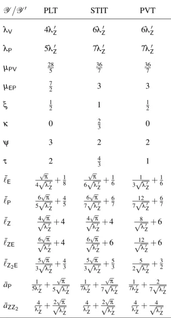
Concluding the paper we will give three examples for column tessellations. The generating planar tessellations are the Poisson line tessellation (PLT), the STIT tessellation and the Poisson- Voronoi tessellation (PVT), respectively. We will consider the column tessellations with constant cell height 1 (ρZ=1) and we restrict for the planar mosaics to the stationary and isotropic case. The intensities, topological/ interior parameters and metric mean values for those column tessellations are presented in Table 2. To facilitate the comparability of the results we assume that all the underlying planar tessellations have the same cell-intensityλ_Z0. In Table 1 the seven necessary parameters of the planar PLT, STIT and PVT are given (Chiu et al., 2013; Nagel and Weiss, 2008). In a PLT all vertices have 4 emanating edges (µ_VE0 =4, µ_VE0(2) =

16), whereas in STIT and PVT all vertices have 3 emanating edges (µ_VE0 =3, µ_VE0(2)=9). PLT and PVT

are side-to-side (φ=µ_EV0 _[π]=0); a STIT tessellation is

non side-to-side and all vertices areπ-vertices (φ=1, µ_EV0 _[π] =2). Through the paper all our results were considered for the special case of a column tessellation with constant height 1. In Remark 3.3 the α-, β

-andγ-mean values are given, Remark 4.3 presents the

intensities and topological/interior mean values and the metric mean values are given in the previous section. Using those results the entries in Table 2 and other interesting quantities of those column tessellations can be computed.

Table 1.Seven parameters of the planar tessellation.

Y0 _{PLT STIT PVT}

λ_V0 λ_Z0 2λ_Z0 2λ_Z0

µ_VE0 4 3 3

µ_VE0(2) 16 9 9

φ 0 1 0

µ_EV0 _[π] 0 2 0

¯ `0_E

√

π

2√λ_Z0

√

π

3√λ_Z0

2 3√λ_Z0

¯

a0_Z 1

λ_Z0

1

λ_Z0

1

λ_Z0

Table 2. Fifteen mean values of the corresponding column tessellation with height1.

Y

Y0 _{PLT STIT PVT}

λV 4λZ0 6λZ0 6λZ0

λP 5λ_Z0 7λ_Z0 7λ_Z0

µPV 28₅ 36₇ 36₇

µEP 7₂ 3 3

ξ 1₂ 1 1₂

κ 0 2₃ 0

ψ 3 2 2

τ 2 4₃ 1

¯ `E

√

π

4√λ_Z0 +

1 8

√

π

6√λ_Z0 +

1 6

1 3√λ_Z0 +

1 6

¯

`P 6

√

π

5√λ_Z0 +

4 5

6√π

7√λ_Z0 +

6 7

12 7√λ_Z0 +

6 7

¯

`Z 4

√

π

√

λ_Z0 +4

4√π

√

λ_Z0 +4

8

√

λ_Z0 +6

¯

`ZE 6

√

π

√

λ_Z0 +4

6√π

√

λ_Z0 +6

12

√

λ_Z0 +6

¯ `Z2E

5√π

3√λ_Z0 +

4 3

5√π

3√λ_Z0 +

5 3

5 2√λ_Z0 +

3 2

¯

aP _5λ10

Z

+

√

π

5√λ_Z0

1 7λ_Z0 +

√

π

7√λ_Z0

1 7λ_Z0 +

2 7√λ_Z0

¯

a_ZZ2 4

λ_Z0 +

2√π

√

λ_Z0

4

λ_Z0 +

2√π

√

λ_Z0

4

λ_Z0 +

4

√

λ_Z0

ACKNOWLEDGEMENT

We thank the two referees for their helpful comments. The first two authors were supported by the German research foundation (DFG), grant WE 1799/3-1.

REFERENCES

Chiu SN, Stoyan D, Kendall WS, Mecke J (2013). Stochastic geometry and its applications. 3rd Ed. Chichester: Wiley.

Cowan R (2013). Line segments in the isotropic planar STIT tessellation. Adv Appl Probab 45:295–311.

Cowan R, Weiss V (2015). Constraints on the fundamental topological parameters of spatial tessellations. Math Nachr 288:540–65.

Gr¨unbaum B, Shephard GC (1987). Tilings and Patterns. New York: WH Freeman.

Mecke J (1984). Parametric representation of mean values for stationary random mosaics. Math Operationsforsch Statist Ser Statist 15:437–42.

Mecke J, Nagel W, Weiss V (2008). The iteration of random tessellations and a construction of a homogeneous process of cell divisions. Adv Appl Probab 40:49–59. Møller J (1989). Random tessellations in Rd. Adv Appl

Probab 21:37–73.

Mosser LJ, Matth¨ai SK (2014). Tessellations stable under iteration – Evaluation of application as an improved stochastic discrete fracture modeling algorithm. Proc Int Discrete Fracture Network Eng Conf. Oct 19–22. Vancouver.

Nagel W, Weiss V (2005). Crack STIT tessellations

– characterization of stationary random tessellations stable with respect to iteration. Adv Appl Probab 37:859–83.

Nagel W, Weiss V (2008). Mean values for homogeneous STIT tessellations in 3D. Image Anal Stereol 27:29–37. Radecke W (1980). Some mean-value relations on stationary random mosaics in the space. Math Nachr 97:203–10.

Schneider R, Weil W (2008). Stochastic and integral geometry. Berlin: Springer.

Th¨ale C, Weiss V (2013). The combinatorial structure of spatial STIT tessellations. Discrete Comput Geom 50:649–72.

Th¨ale C, Weiss V, Nagel W (2012). Spatial STIT tessellations: Distributional results for I-segments. Adv Appl Probab 44:1–20.