ISSN: 1311-1728 (printed version); ISSN: 1314-8060 (on-line version) doi:http://dx.doi.org/10.12732/ijam.v32i2.13
PRIMAL-DUAL ALGORITHMS FOR SEMIDEFINITE OPTIMIZATION PROBLEMS BASED ON KERNEL-FUNCTION
WITH TRIGONOMETRIC BARRIER TERM Mohamed El Ghami1§, Guoqiang Wang2, Trond Steihaug3
1Nord University Faculty of Education and Arts
Nesna 8700, NORWAY 2College of Fundamental Studies Shanghai University of Engineering Science
Shanghai 201620, P.R. CHINA 3University of Bergen Department of Informatics Box 7803, N-5020, Bergen, NORWAY
Abstract: In this paper we extended the results obtained for the first trigono-metric kernel-function-based IPMs introduced by El Ghami et al. in [8] for LO to semidefinite optimization problems. The kernel function has a trigonomet-ric Barrier Term. In this paper we generalize the analysis presented in the above paper for Semidefinit Optimization Problems (SDO). It is shown that the interior-point methods based on this function for large-update methods, the iteration bound is improved significantly. For small-update interior point methods the iteration bound is the best currently known bound for primal-dual interior point methods. The analysis for SDO deviates significantly from the analysis for linear optimization. Several new tools and techniques are derived in this paper.
AMS Subject Classification: 90C22, 90C31
Key Words: kernel function, interior-point, semidefinite optimization, primal-dual method
1. Introduction
Since the path-breaking paper of Karmarkar, linear optimization (LO) revived as an active area of research. Today the resulting interior-point methods (IPMs) are among the most effective methods for solving wide classes of LO problems. Many researchers have proposed and analyzed various IPMs for LO and a large amount of results have been reported. For a survey we refer to recent books on the subject [9, 12, 14, 15, 20] and the references cited their in.
In the literature two types of primal-dual IPMs are distinguished: large-update methods and small-large-update methods, according to the value of the barrier-update parameter θ. However, there is still a gap between the prac-tical behavior of these algorithms and these theoreprac-tical performance results. The so-called large-update IPMs have superior practical performance but with relatively weak theoretical results. While the so-called small-update IPMs enjoy the best known worst-case iteration bounds but their performance in computa-tional practice is poor.
In the last twenty years, this gap was reduced significantly by Peng et al. [15] who introduced the so-called self-regular kernel functions and designed primal-dual IPMs based on self-regular proximities for LO. They improved the iteration bound for large-update methods fromO(nlognε) toO(√nlognlognε), which almost closes the gap between the iteration bounds for large- and small-update methods. Later, Bai, et al. [4] presented a large class of eligible kernel functions, which is fairly general and includes the classical logarithmic function and the self-regular functions, as well as many non-self-regular functions as special cases. The best known iteration bounds for LO obtained are as good as the ones in [15] for appropriate choices of the eligible kernel functions.
Particularly, El Ghami et al. [8] first introduced a trigonometric kernel function for primal-dual IPMs in LO. They established the worst case iter-ation bounds for large- and small-update methods, namely, O(n34 logn
ε) and O(√nlognε), respectively. In[6, 13] the authors proposed a primal-dual interior-point algorithm for SDO and for P∗(κ)-Linear Complementarity problems [7] based on a different kernel function with trigonometric barrier term and ob-tained the same iteration bounds as for LO.
We consider the standard semidefinite optimization problem (SDO)
(SDP) p∗ = inf
and its dual problem (SDD)
(SDD) d∗= sup
y,S
(
bTy:
m
X
i=1
yiAi+S =C, S 0 )
,
where C and Ai are symmetric n×n matrices, b, y ∈ Rm, and X 0 means
thatXis symmetric positive semidefinite and Tr(A) denotes the trace ofA(i.e., the sum of its diagonal elements). Without loss of generality the matrices Ai
are assumed to be linearly independent. Recall that for any twon×nmatrices,
A and B their natural inner product is given by
Tr(ATB) =
n
X
i=1
n
X
j=1
AijBij.
IPMs provide a powerful approach for solving SDO problems. A comprehen-sive list of publications on SDO can be found in the SDO homepage maintained by Alizadeh [1]. Pioneering works are due to Alizadeh [1, 2] and Nesterov et al. [12]. Most IPMs for SDO can be viewed as natural extensions of IPMs for linear optimization (LO), and have similar polynomial complexity results. However, to obtain valid search directions is much more difficult than in the LO case. In the sequel we describe how the usual search directions are ob-tained for primal-dual methods for solving SDO problems. Our aim is to show that the kernel-function-based approach that we presented for LO in [8] can be generalized and applied also to SDO problems.
1.1. Classical search direction
We assume that (SDP) and (SDD) satisfy the interior-point condition (IPC), i.e., there exists X0 ≻ 0 and (y0, S0) with S0 ≻ 0 such that X0 is feasible for (SDP) and (y0, S0) is feasible for (SDD). Moreover, we may assume that
X0 = S0 =E, where E is then×n identity matrix [14]. Assuming the IPC, one can write the optimality conditions for the primal-dual pair of problems as follows.
Tr(AiX) = bi, i= 1, . . . , m m
X
i=1
yiAi+S = C (1)
XS = 0
The basic idea of primal-dual IPMs is to replace the complementarity condition
XS= 0 by the parameterized equation
XS=µE; X, S ≻0,
where µ >0. The resulting system has a unique solution for each µ >0. This solution is denoted by (X(µ), y(µ), S(µ)) for each µ > 0; X(µ) is called the
µ-center of (SDP) and (y(µ), S(µ)) is the µ-center of (SDD). The set of µ -centers (with µ >0) defines a homotopy path, which is called the central path of (SDP) and (SDD) [14, 15]. The principal idea of IPMs is to follow this central path and approach the optimal set asµgoes to zero. Newton’s method amounts to linearizing the system (1), thus yielding the following system of equations.
Tr(Ai∆X) = 0, i= 1, . . . , m m
X
i=1
∆yiAi+ ∆S = 0 (2)
X∆S+ ∆XS = µE−XS.
This so-called Newton system has a unique solution (∆X,∆y,∆S). Note that ∆Sis symmetric, due to the second equation in (2). However, a crucial point is that ∆X may be not symmetric. Many researchers have proposed various ways of ‘symmetrizing’ the third equation in the Newton system so that the new system has a unique symmetric solution. All these proposals can be described by using a symmetric nonsingular scaling matrixP and by replacing (2) by the system
Tr(Ai∆X) = 0, i= 1, . . . , m m
X
i=1
∆yiAi+ ∆S = 0 (3)
∆X+P∆SPT = µS−1−X
Now ∆X is automatically a symmetric matrix.
1.2. Nesterov-Todd direction
In this paper we consider the symmetrization schema of Nesterov-Todd [16]. So we use
P =X12
X12SX 1 2
−1 2
X12 =S− 1 2
S12XS 1 2
1 2
where the last equality can be easily verified. Let D=P12, where P 1
2 denotes
the symmetric square root of P. Now, the matrix D can be used to scale X
and S to the same matrix V, namely [14, 17]:
V := √1
µD
−1XD−1 = √1
µDSD. (4)
Obviously the matrices D and V are symmetric, and positive definite. Let us further define
¯
Ai := √1
µDAiD, i= 1,2, . . . , m;
and
DX :=
1
√µD−1∆XD−1; DS :=
1
√µD∆SD. (5)
We refer toDX andDSas the scaled search directions. Now (3) can be rewritten as follows:
Tr( ¯AiDX) = 0, i= 1, . . . , m. m
X
i=1
∆yiAi¯ +DS = 0, (6)
DX +DS = V−1−V.
In the sequel, we use the following notational conventions. Throughout this paper, k·k denotes the 2-norm of a vector. The nonnegative and the positive orthants are denoted as Rn+ and intRn+, respectively, and Sn
, Sn
+, and intSn+ denote the cone of symmetric, symmetric positive semidefinite and symmetric positive definiten×nmatrices, respectively. For anyV ∈Sn, we denote byλ(V) the vector of eigenvalues of V arranged in increasing order, λ1(V)≤ λ2(V)≤
, . . . , λn(V). For any square matrix A, we denote byη1(A)≤η2(A)≤, . . . ,≤
ηn(A) the singular values ofA; ifAis symmetric, then one hasηi(A) =|λi(A)|, i= 1,2, . . . , n.If z∈Rn and f :R→R, then f(z) denotes the vector in Rn whosei-th component is f(zi), with 1≤i≤n, and ifD is a diagonal matrix, then f(D) denotes the diagonal matrix with f(Dii) as i diagonal component. For X ∈Sn, X =Q−1DQ, where Q is orthogonal, and D a diagonal matrix,
2. New search direction
In this section we introduce the new search direction. But we start with the definition of a matrix function [18, 19].
Definition 1. Let X be a symmetric matrix, and let
X=Q−1X diag(λ1(X), λ2(X), . . . , λn(X))QX,
be an eigenvalue decomposition of X, whereλi(X), 1≤i≤ndenotes the i-th eigenvalue ofX, andQX is orthogonal. Ifψ(t) is any univariate function whose domain contains {λi(X); 1≤i≤n} then the matrix function ψ(X) is defined by
ψ(X) =Q−1X diag(ψ(λ1(X)), ψ(λ2(X)), . . . , ψ(λn(X)))QX.
and the scalar function Ψ(X) is defined as follows [15]:
Ψ(X) :=
n
X
i=1
ψ(λi(X)) = Tr(ψ(X)). (7)
The univariate functionψis called the kernel function of the scalar function Ψ.
In this paper, when we use the function ψ(·) and its first three derivatives
ψ′(·), ψ′′(·), and ψ′′′(·) without any specification, it denotes a matrix function if the argument is a matrix and a univariate function (from R to R) if the argument is in R.
Analogous to the case of LO, the kernel-function-based approach to SDO is obtained by modifying Nesterov-Todd direction [15].
The observation underlying our approach is that the right-hand sideV−1−V
in the third equation of (6) is precisely −ψ′(V) ifψ(t) = (t2−1)/2−logt, the latter being the kernel function of the well-known logarithmic barrier function. Note that this kernel function is strictly convex and nonnegative, whereas its domain contains all positive reals and it vanishes at 1. As we will now show any continuously differentiable kernel function ψ(t) with these properties gives rise to a primal-dual algorithm for SDO.
Given such a kernel functionψ(t) we replace the right-hand sideV−1−V in the third equation of (6) by−ψ′(V), withψ′(V) defined according to Definition 1. Thus we use the following system to define the (scaled) search directionsDX
an DS:
m
X
i=1
∆yiAi¯ +DS = 0 (8)
DX +DS = −ψ′(V).
Having DX and DS, △X and △S can be calculated from (5). Due to the orthogonality of △X and △S, it is trivial to see thatDX⊥DS, and so
Tr(DXDS) = Tr(DSDX) = 0. (9)
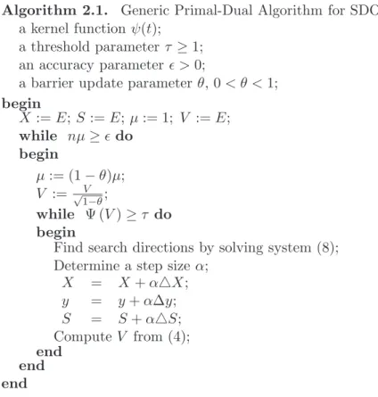
The algorithm considered in this paper is described in Figure 1.
Algorithm 2.1. Generic Primal-Dual Algorithm for SDOInput: a kernel functionψ(t);
a threshold parameterτ ≥1; an accuracy parameterǫ >0;
a barrier update parameterθ,0< θ <1; begin
X:=E;S:=E;µ:= 1; V :=E; while nµ≥ǫdo
begin
µ:= (1−θ)µ;
V := √V 1−θ;
while Ψ (V)≥τ do begin
Find search directions by solving system (8); Determine a step size α;
X = X+α△X;
y = y+α∆y;
S = S+α△S; ComputeV from (4); end
end end
Figure 1: Generic primal-dual interior-point algorithm for SDO.
S =E. Since then XS =µE for µ= 1 it follows from (4) thatV =E at the start of the algorithm, whence Ψ(V) = 0. We then decreaseµto µ:= (1−θ)µ, for some θ ∈(0,1). In general this will increase the value of Ψ(V) above the threshold value τ. To get this value smaller again, and coming closer to the current µ-center, we solve the scaled search directions from (8), and unscale these directions by using (5). By choosing an appropriate step sizeα, we move along the search direction, and construct a new triple (X+, y+, S+) with
X+=X+α△X y+=y+α∆y S+=S+α△S. (10)
If necessary, we repeat the procedure until we find iterates such that Ψ(V) no longer exceed the threshold value τ, which means that the iterates are in a small enough neighborhood of (X(µ), y(µ), S(µ)). Then µis again reduced by the factor 1−θand we apply the same procedure targeting at the newµ-centers. This process is repeated untilµis small enough, i.e. untilnµ≤ǫ. At this stage we have found anǫ-solution of (SDP) and (SDD). Just as in theLOcase, the parameters τ, θ, and the step size α should be chosen in such a way that the algorithm is ‘optimized’ in the sense that the number of iterations required by the algorithm is as small as possible. Obviously, the resulting iteration bound will depend on the kernel function underlying the algorithm, and our main task becomes to find a kernel function that minimizes the iteration bound.
The rest of the paper is organized as follows. In Section 3 we introduce the kernel function ψ(t) considered in this paper and discuss some of its properties that are needed in the analysis of the corresponding algorithm. In Section 4 we derive the properties of the barrier function Ψ(V). The step size α and the resulting decrease of the barrier function are discussed in Section 5. The total iteration bound of the algorithm and the complexity results are derived in Section 6. Finally, some concluding remarks follow in Section 7.
3. Our kernel function and some of its properties
Recently in [5, 8] investigated new kernel functions with trigonometric barrier for LO. In [13] the author present a primal-dual interior-point algorithm for SDO based on kernel function
ψ(t) = t 2−1
2 + 4
πcot (h(t)), with h(t) = πt
1 +t. (11)
In this paper we consider kernel functions of the form
ψ(t) = t 2−1
2 + 6
π tan (h(t)), with h(t) =
π(1−t)
and to show that the interior-point methods for SDO based on these function have favorable complexity results.
Note that the growth term of our kernel function is quadratic. However, this function (12) deviates from all other kernel functions since its barrier term is trigonometric as 6πtanπ4(1−t+2t). In order to study the new kernel function, several new arguments had to be developed for the analysis.
This section is started by technical lemma, and then some properties of the new kernel function introduced in this paper are derived.
3.1. Some technical results
In the analysis of the algorithm based onψ(t) we need its first three derivatives. These are given by
ψ′(t) = t+6h′(t)
π 1 + tan
2(h(t)), (13)
ψ′′(t) = 1 + 6
π 1 + tan
2(h(t)) h′′(t) + 2h′(t)2tan(h(t)). (14)
ψ′′′(t) = 6
π 1 + tan
2(h(t))k(t), (15)
with
k(t) := 6h′′(t)h′(t) tan(h(t)) +h′′′(t) + 2h′(t)3 3 tan2(h(t)) + 1. (16)
The next lemma serves to prove that the new kernel function (12) is eligible.
Lemma 2. [Lemma 2 in [8]]Letψbe as defined in (12) andt >0. Then,
ψ′′(t) > 1, (17-a)
tψ′′(t) +ψ′(t) > 0, (17-b)
tψ′′(t)−ψ′(t) > 0, (17-c)
and ψ′′′(t) < 0. (17-d)
It follows that ψ(1) = ψ′(1) = 0 andψ′′(t) ≥0, proving that ψ is defined by ψ′′(t).
ψ(t) = Z t
1 Z ξ
1
ψ′′(ζ)dζdξ. (18)
z 7→ ψ(ez) and this holds if and only if ψ(√t
1t2) ≤ 12(ψ(t1) +ψ(t2)) for any
t1, t2 ≥ 0. Following [3], we therefore say that ψ is exponentially convex, or shortly,e-convex, whenevert >0.
Lemma 3. Letψ be as defined in (12), one has
ψ(t)< 1
2ψ
′′(1) (t−1)2, if t >1.
Proof. By Taylor’s theorem and ψ(1) =ψ′(1) = 0,we obtain
ψ(t) = 1 2ψ
′′(1) (t−1)2+1 6ψ
′′′(ξ) (ξ−1)3,
where 1< ξ < tif t >1. Since ψ′′′(ξ)<0,the lemma follows.
Lemma 4. Letψ be as defined in (12), one has
tψ′(t)≥ψ(t), if t≥1.
Proof. Definingg(t) :=tψ′(t)−ψ(t) one has g(1) = 0 andg′(t) =tψ′′(t)≥
0.Hence g(t)≥0 and the lemma follows.
At some places below we apply the function Ψ to a positive vector v. The interpretation of Ψ(v) is compatible with Definition 1 when identifying the vector v with its diagonal matrix diag (v). When applying Ψ to this matrix we obtain
Ψ(v) =
n
X
i=1
ψ(vi), v∈intRn+.
4. Properties of Ψ(V) and δ(V)
In this section we extend Theorem 4.9 in [4] to the cone of positive definite matrices.
The next theorem gives a lower bound on the norm-based proximity measure
δ(V), defined by
δ(V) = 12kψ′(V)k= 1 2
v u u t
n
X
i=1
ψ′(λi(V))2 = 1
in terms of Ψ(V). Since Ψ(V) is strictly convex and attains its minimal value zero at V =E, we have
Ψ (V) = 0 ⇔ δ(V) = 0 ⇔ V =E.
We denote by ̺ : [0,∞) → [1,∞) the inverse function of ψ(t) for t ≥ 1. In other words,
s=ψ(t) ⇔ t=̺(s), t≥1. (20)
Theorem 5. Let ̺ be as defined in (20). Then
δ(V)≥ 12ψ′(̺(Ψ(V))).
Proof. IfV =E thenδ(V) = Ψ(V) = 0. Since̺(0) = 1 andψ′(1) = 0, the
inequality holds with equality ifV =E. Otherwise, by the definitions ofδ(V) in (19) and Ψ(V) in (7), we have δ(V) > 0 and Ψ(V) > 0. Let vi := λi(V), 1≤i≤n. Then v >0 and
δ(V) =12 v u u t
n
X
i=1
ψ′(λi(V))2 = 1 2
v u u t
n
X
i=1
ψ′(vi)2.
Since ψ(t) satisfies (17-d) we may apply Theorem 4.9 in [4] to the vector v. This gives
δ(V)≥ 12ψ′ ̺ n
X
i=1
ψ(vi) !!
.
Since
n
X
i=1
ψ(vi) =
n
X
i=1
ψ(λi(V)) = Ψ(V),
the proof of the theorem is complete.
Lemma 6. IfΨ(V)≥1,then
δ(V)≥ 1 6Ψ(V)
1
2. (21)
Proof. The proof of this lemma uses Theorem 5 and Lemma 4. Putting
s= Ψ(V), we obtain from Theorem 5 that
Puttingt=̺(s), we have by (20),
ψ(t) = t 2−1
2 + 6
πtan (h(t)) =s, with h(t) =
π(1−t)
4t+ 2 , t≥1.
Fort≥1 we have−π4 ≤h(t) = π4(1−t+2t) <0 which implies that−1≤tan (h(t))<
0 for allt∈]1,∞], using s, t≥1 we get
t2−1 2 =s−
6
π tan (h(t))≤s+
6
π ≤s+ 2≤3s,
whence
t2 ≤1 + 6s≤7s,
and therefore,
̺(s) =t≤√7s≤3s12.
Now applying Lemma 4 we may write
δ(V)≥ 1 2ψ
′(̺(s))≥ ψ(̺(s)) 2̺(s) =
s
2̺(s) ≥ 1 6s
1
2 = 1
6Ψ(V)
1 2.
This proves the lemma.
Note that since τ ≥ 1 we have at the start of each inner iteration that Ψ(V)≥1.Substitution in (21) gives
δ(V)≥ 1
6. (22)
5. Analysis of the algorithm
In the analysis of the algorithm the concept of exponential convexity [4, 9] is again a crucial ingredient. In this section we derive a default value for the step size and we obtain an upper bound for the decrease in Ψ(V) during a Newton step.
Lemma 7. Let A, B∈Sn be two nonsingular matrices andf(t) be given
real-valued function such that f(et) is a convex function. One has
n
X
i=1
f(ηi(AB))≤ n
X
i=1
f(ηi(A)ηi(B)),
where ηi(A), and ηi(B) i = 1,2, ..., n denote the singular values of A and B
respectively
Lemma 8. LetA, A+B ∈Sn+, then one has
λi(A+B)≥λ1− |λn(B)|, i= 1,2, ..., n.
Proof. It is obvious that λi(A+B) ≥ λ1(A+B). By the Rayleigh-Ritz
theorem (see [11]), there exists a nonzeroX0 ∈Rn, such that
λ1(A+B) =
XT
0(A+B)X0
XT
0X0
= X
T
0AX0
XT
0 X0 +X
T
0 BX0
XT
0X0
.
We therefore may write
λ1(A+B) ≥
X0TAX0
XT
0 X0 −
X0TBX0
XT
0 X0 ≥ min X6=0
XTAX
XTX −maxX6=0
XTBX XTX
=λ1− |λn(B)|.
This completes the proof of the lemma.
A consequence of condition (17-b) is that any eligible kernel function is exponentially convex [15, Eq. (2.10)]:
ψ(√t1t2)≤ 1
2(ψ(t1) +ψ(t2)), ∀t1 >0,∀t2>0. (23) This implies the following lemma, which is crucial for our purpose.
Lemma 9. Let V1 and V2 be two symmetric positive definite matrices,
then Ψ (V 1 2
1 V2V
1 2 1 ) 1 2
≤ 12(Ψ(V1) + Ψ(V2)), ∀V1 ≻0,∀V2 ≻0.
Proof. For any nonsingular matrix U ∈Sn,we have
ηi(U) = λi(UTU)
1 2
= λi(U UT)
1 2
Taking U =V 1 2 1 V 1 2
2 , we may write
ηi(V
1 2
1 V
1 2
2 ) =
λi(V
1 2
1 V2V
1 2 1 ) 1 2 =λi (V 1 2
2 V1V
1 2
2 ) 1
2
, i= 1,2, ..., n.
Since V1 and V2 are symmetric positive definite, using Lemma 7 one has
Ψ
(V
1 2
1 V2V
1 2 1 ) 1 2 = n X i=1 ψ
ηi(V
1 2 1 V 1 2 2 ) ≤ n X i=1 ψ
ηi(V
1 2
1 )ηi(V
1 2
2 )
.
Sinceη1(V
1 2
1 ), η1(V
1 2
2 )>0 we may use thatψ(t) satisfies (17-b) fort >0. Using (23), hence we obtain
Ψ
(V
1 2
1 V2V
1 2 1 ) 1 2 ≤ 1 2 n X i=1 ψ
η2i(V
1 2 1 ) +ψ
η2i(V
1 2 2 ) = 1 2 n X i=1
(ψ(λi(V1)) +ψ(λi(V2)))
= 1
2(Ψ(V1) + Ψ(V2)). This completes the proof.
5.2. The decrease of the proximity in the inner iteration In this subsection we are going to compute a default value for the step size α
in order to yield a new triple (X+, y+, S+) as defined in (10). After a damped step, using (5) we have
X+ = X+α△X =X+α√µDDXD=√µD(V +αDX)D,
y+ = y+α∆y,
S+ = S+α△S=X+α√µD−1DSD1 =√µD−1(V +αDS)D−1.
Denoting the matrixV after the step asV+, we have
V+= 1
√µ D−1X+S+D 1
2
.
Note thatV2
+ is unitarily similar to the matrix µ1X
1 2
+S+X
1 2
+ and hence also to
(V +αDX)
1
This implies that the eigenvalues of V+ are the same as those of the matrix
˜
V+ :=
(V +αDX)12 (V +αDS) (V +αDX) 1 2
1 2
.
The definition of Ψ(V) implies that its value depends only on the eigenvalues of V. Hence we have
ΨV˜+
= Ψ (V+).
Our aim is to find α such that the decrement
f(α) := Ψ (V+)−Ψ (V) = Ψ
˜
V+
−Ψ (V), (24)
is as small as possible. Due to Lemma 9, it follows that
ΨV˜+
= Ψ(V +αDX)12(V +αDS) (V +αDX) 1 2
1 2
≤ 12[Ψ (V +αDX) + Ψ (V +αDS)].
From the definition (24) of f(α), we now havef(α)≤f1(α), where
f1(α) := 12[Ψ (V +αDX) + Ψ (V +αDS)]−Ψ (V).
Note thatf1(α) is convex inα, since Ψ is convex. Obviously,f(0) =f1(0) = 0. Taking the derivative with respect toα, we get
f1′(α) = 12Tr ψ′(V +αDX)DX+ψ′(V +αDS)DS.
Using the last equality in (8) and also (19), this gives
f1′(0) = 12Tr ψ′(V) (DX +DS)
=−12Tr ψ′(V)2=−2δ(V)2.
Differentiating once more, we obtain
f1′′(α) = 12Tr ψ′′(V +αDX)D2X +ψ′′(V +αDS)D2S
. (25)
In the sequel we use the following notation:
λ1 := min(λi(V)), δ :=δ(V).
Lemma 10. One has
Proof. The last equality in (8) and (19) imply thatkDX +DSk2 =kDXk2+
kDSk2 = 4δ2. Thus we have |λn(DX)| ≤2δ and |λn(DS)| ≤2δ. Using Lemma 8 and V +αDX 0,As a consequence we have, for eachi,
λi(V +αDX) ≥ λ1−α|λn(DX)| ≥λ1−2αδ,
λi(V +αDS) ≥ λ1−α|λn(DS)| ≥λ1−2αδ.
Due to (17-d),ψ′′ is monotonically decreasing. So the above inequalities imply that
ψ′′(λi(V +αDX))≤ψ′′(λ1−2αδ),
ψ′′(λi(V +αDS))≤ψ′′(λ1−2αδ).
Substitution into (25) gives
f1′′(α) ≤ 12ψ′′(λ1−2αδ) Tr D2X +D2S
= 12ψ′′(λ1−2αδ)
kDXk2+kDSk2
.
Now, using that DX and DS are orthogonal, by (9), and also kDX +DSk2 = 4δ2, by (19), we obtain
f1′′(α)≤2δ2ψ′′(λ1(V)−2αδ).
This proves the lemma.
Using the notation vi =λi(V), 1≤i≤n, again, we have
f1′′(α)≤2δ2ψ′′(v1−2αδ), (26)
which is exactly the same inequality as Lemma 3.1 in [8]. This means that our analysis closely resembles the analysis of the LO case in [8]. From this stage on we can apply similar arguments as in the LO case. In particular, the following two lemmas can be stated without proof.
Lemma 11. [Lemmas 3.3 and 3.4 in [10]]Letρ be the inverse function of
−12ψ′(t) for t∈(0,1]. Then the largest value of the step size α satisfying (26)
is given by
ˆ
α:= 1
2δ[ρ(δ)−ρ(2δ)].
Moreover,
ˆ
α≥ 1
For future use we define
e
α:= 1
ψ′′(ρ(2δ)). (27)
By Lemma 11 this step size satisfies (26).
Lemma 12. If the step size α is such that α≤αˆ then
f(α)≤ −α δ2.
Using the above lemmas from [8] we proceed as follows.
Theorem 13. Let ρ be as defined in Lemma 11 and αe as in (27) and
Ψ(v)≥1. Then
f(˜α)≤ − δ 2
ψ′′(ρ(2δ)) ≤ −
δ12
2593.
Proof. Since αe ≤ α,ˆ Lemma 12 gives f(αe) ≤ −α δe 2, where αe = ψ′′(ρ1(2δ))
as defined in (27). Thus the first inequality follows. To obtain the inverse functiont=ρ(s) of−12ψ′(t) for t∈(0,1], we need to solvetfrom the equation
−t+6hπ′(t) 1 + tan2(h(t))= 2s. This implies,
1 + tan2(h(t)) = −π
6h′(t)(2s+t)
= 2π(2t+ 1) 2
18π (2s+t)≤2s+ 1 for t≤1.
Hence, puttingt=ρ(2δ),which is equivalent to 4δ=−ψ′(t),we get
tan(h(t))≤2√δ. (28)
Using (28), thus we have
e
α= 1
ψ′′(t) =
1
1 + π6 (1 + tan2(h(t))) (h′′(t) + 2h′(t)2tan(h(t)))
≥ 1
Since h′′(t) = 6π
(2t+1)3 ≤6π, andh′(t)2 = 9
π2
4(2t+1)4 ≤ 9
π2
4 for all 0 ≤t≤1.Then we have
e
α≥ 1
1 +π6 (1 + 4δ)6π+ 9π2√δ =
1
1 + 18 (1 + 4δ)2 + 3π√δ .
Also using (22) (i.e., 6δ≥1) we get,
e
α ≥ 1
(6δ)32 + 18 (6δ+ 4δ)
2√6δ+ 3π√δ
= 1
632 + 180 2√6 + 3πδ 3 2
≥ 1
2593δ32
.
Hence
f(αe)≤ − δ 2
ψ′′(ρ(2δ)) ≤ −
δ2
2593δ32
=− δ
1 2
2593.
Thus the theorem follows. Substitution in (21) gives
f(˜α)≤ − δ
1 2
2593 ≤ − Ψ41
2593√6 ≤ − Ψ14
6532.
5.3. A uniform upper bound for Ψ
In this subsection we extend Theorem 3.2 in [4] to the cone of positive definite matrices. As we will see the proof of the next theorem easily follows from Theorem 3.2 in [4].
Theorem 14. Let ̺be as defined in (20). Then for any positive vector v
and any β >1we have:
Ψ(βV)≤nψ
β̺
Ψ(V)
n
.
Proof. Letvi :=λi(V), 1≤i≤n. Then v >0 and
Ψ(βV) =
n
X
i=1
ψ(λi(βV)) =
n
X
i=1
ψ(βλi(V)) =
n
X
i=1
Due to the fact thatψ(t) satisfies (17-c), at this stage we may use Theorem 3.2 in [4], which gives
Ψ(βv) ≤ nψ
β̺
Ψ(v)
n
.
Since
Ψ(v) =
n
X
i=1
ψ(vi) = n
X
i=1
ψ(λi(V)) = Ψ(V),
the theorem follows.
Before the update of µ we have Ψ(V) ≤ τ, and after the update of µ to (1−θ)µ we have V+ = √1−V θ. Application of Theorem 14, with β = √1−1 θ, yields that
Ψ(V+)≤nψ ̺ τ n
√
1−θ
!
.
Therefore we define
L=L(n, θ, τ) :=nψ ̺ τ n
√
1−θ
!
(29)
In the sequel the value L(n, θ, τ) is simply denoted as L. A crucial (but triv-ial) observation is that during the course of the algorithm the value of Ψ(V) will never exceed L, because during the inner iterations the value of Ψ always decreases.
6. Complexity
We are now ready to derive the iteration bounds for large-update methods. An upper bound for the total number of (inner) iterations is obtained by multiply-ing an upper bound for the number of inner iterations between two successive updates ofµ by the number of barrier parameter updates. The last number is bounded above by (cf. [20, Lemma II.17, page 116])
1
θlog n ǫ.
The following lemma is taken from Proposition 1.3.2 in [15]. Its relevance is due to the fact that the barrier function values between two successive updates of µ yield a decreasing sequence of positive numbers. We will denote this sequence as Ψ0,Ψ1, . . ..
Lemma 15. Lett0, t1,· · ·, tK be a sequence of positive numbers such that tk+1≤tk−κt1−k γ, k= 0,1,· · · , K−1,
whereκ >0 and 0< γ≤1. Then K≤jtγ0
κγ
k
.
Lemma 16. If K denotes the number of inner iterations between two
successive updates of µ, then
K ≤ 26128
3 Ψ
3 4
0 ≤8710Ψ
3 4
0.
Proof. The definition of K implies ΨK−1 > τ and, according to Theorem
13, ΨK ≤τ and
Ψk+1≤Ψk−κ(Ψk)1−γ, k= 0,1,· · · , K−1,
with κ = 65321 and γ = 34. Application of Lemma 15, with tk = Ψk yields the
desired inequality.
Usingψ0 ≤L, where the number Lis as given in (29), and Lemma 16 we obtain the following upper bound on the total number of iterations:
8710L34
θ log
n
ǫ. (30)
6.1. Large-update
The inverse function of ψ(t) for t∈[1,∞) is obtained by solving tfrom
ψ(t) = t 2−1
2 + 6
πtan
π(1−t)
4t+ 2 =s, t≥1.
We derive an upper bound fort, as this suffices for our goal. One has from (18) and ψ′′(t)≥1,
s=ψ(t) = Z t
1 Z ξ
1
ψ′′(ζ)dζdξ≥
Z t
1 Z ξ
1
dζdξ= 1 2(t−1)
which implies
t=̺(s)≤1 +√2s. (31)
We just established that (30) is an upper bound for the total number of iterations, using
ψ(t) = t 2−1
2 + 6
πtan
π(1−t) 4t+ 2 ≤
t2−1
2 , for t≥1, and (31), by substitution in (29) we obtain
L≤n
̺(τ n) √ 1−θ 2 −1 2 ≤ n
2 (1−θ)
θ+ 2 r 2τ n + 2τ n
= θn+ 2
√
2τ n+ 2τ
2 (1−θ) . Using (30), thus the total number of iterations is bounded above by
K θ log
n ǫ ≤
8710
θ2 (1−θ)34
θn+ 2√2τ n+ 2τ
3 4
logn
ǫ.
A large-update methods uses τ = O(n) and θ = Θ(1). The right-hand side expression is then On34logn
ǫ
,as easily may be verified.
6.2. Small-update methods For small-update methods one has τ = O(1) and θ= Θ√1n
. Using Lemma 3, withψ′′(1) = 2π9+9,we then obtain
L≤ n(2π+ 9)
18
ρ nτ √
1−θ−1
!2
.
Using (31), then
L≤ n(2π+ 9)
18 1 +
q 2τ
n √
1−θ −1
2
.
Using 1−√1−θ= 1+√θ
1−θ ≤θ, this leads to L≤
(2π+9) 18(1−θ) θ
√
n+√2τ2. We conclude that the total number of iterations is bounded above by
K θ log
n ǫ ≤
8710 (2π+ 9)34
θ(18 (1−θ))34
θ√n+√2τ
3 2
logn
ǫ.
Thus the right-hand side expression is then O √nlogn ǫ
7. Concluding Remarks
In this paper we extended the results obtained for kernel-function-based IPMs in [8] for LO to semidefinite optimization problems. The analysis in this paper is new and different from the one using forLO. Several new tools and techniques are derived in this paper. The proposed function has a trigonometric barrier term but the function is not logarithmic and not self- regular. We proved that the iteration bound of a large-update interior-point method based on the kernel function considered in this paper isOn34 logn
ǫ
,which is the same complexity achieved in [13] by using a different trigonometric kernel function (11). The obtained complexity improves the classical iteration complexity with a factor
n14. For small-update methods we obtain the best know iteration bound, namely
O √nlognǫ.
References
[1] F. Alizadeh, Combinatorial Optimization with Interior Point Methods and Semi-Definite Matrices, PhD thesis, University of Minnesota, Minneapolis, Minnesota, USA (1991).
[2] F. Alizadeh, Interior point methods in semidefinite programming with ap-plications to combinatorial optimization,SIAM J. on Optimization, 5 No 1 (1995), 13-51.
[3] Y.Q. Bai, M. El Ghami, C. Roos, A new efficient large-update primal-dual interior-point method based on a finite barrier,SIAM J. on Optimization, 13No 3 (2003), 766-782.
[4] Y.Q. Bai, M. El Ghami, C. Roos, A comparative study of kernel functions for primal-dual interior-point algorithms in linear optimization, SIAM J. on Optimization,15No 1 (2004), 101-128.
[5] X.Z. Cai, G.Q.Wang, M. El Ghami, Y.J. Yue, Complexity analysis of primal-dual interior-point methods for linear optimization based on a para-metric kernel function with a trigonopara-metric barrier term, Abstr. Appl. Anal. (2014), Art. # 710158.
[7] M. El Ghami, G.Q. Wang, Interior-point methods forP∗(κ)-linear comple-mentarity problems based on generalised trigonometric barier function. International J. of Applied Mathematics, 30, No 1 (2017), 11-33, doi: 10.12732/ijam.v30i1.2.
[8] M. El Ghami, Z.A. Guennoun, S. Bouali, T. Steihaug, Primal-dual iInterior-point methods for linear optimization based on a kernel function with trigonometric barrier term, J. of Computational and Applied Mathe-matics,236, No 15 (2012), 3613-3623.
[9] M. El Ghami, A Kernel Function Approach for Interior Point Methods: Analysis and Implementation, LAP Lambert Academic Publishing, Ger-many, (2011).
[10] M. El Ghami, C. Roos, Generic primal-dual interior point methods based on a new kernel function, International J. RAIRO-Operations Research, 42, No 2 (2008), 199-213.
[11] R.A. Horn, C.R. Johnson, Topics in Matrix Analysis,Cambridge Univer-sity Press, Cambridge (1991).
[12] Y.E. Nesterov, A.S. Nemirovskii, Interior Point Polynomial Methods in Convex Programming: Theory and Algorithms, SIAM, Philadelphia, USA (1993).
[13] B. Kheirfam, Primal-dual interior-point algorithm for semidenite optimiza-tion based on a new kernel funcoptimiza-tion with trigonometric barrier term, Nu-merical Algorithms,61, No 4 (2012), 659-680.
[14] E. de Klerk, Aspects of Semidefintie Programming: Interior Point Algo-rithms and Selected Applications, Applied Optimization Book 65, Kluwer Academic Publishers, Dordrecht (2002).
[15] J. Peng, C. Roos, T. Terlaky,Self-Regularity: A New Paradigm for Primal-Dual Interior-Point Algorithms, Princeton University Press (2002).
[16] Y.E. Nesterov, M.J. Todd, Self-scaled barriers and interior-point methods for convex programming, Mathematics of Operations Research, 22, No 1 (1997), 1-42.
[18] R.A. Horn, C.R. Johnson, Matrix Analysis, Cambridge University Press, Cambridge, UK (1985).
[19] W. Rudin,Principles of Mathematical Analysis, Mac-Graw Hill Book Com-pany, New York (1978).