An Active Set Algorithm for Robust Combinatorial
Optimization Based on Separation Oracles
C. Buchheim
†and M. De Santis
∗†
Fakult¨at f¨
ur Mathematik
TU Dortmund
Vogelpothsweg 87 - 44227 Dortmund - Germany
∗
Dipartimento di Ingegneria Informatica, Automatica e Gestionale
Sapienza, Universit`
a di Roma
Via Ariosto, 25 - 00185 Roma -Italy
e-mail (Buchheim): [email protected]
e-mail (De Santis): [email protected]
Abstract
We address combinatorial optimization problems with uncertain coefficients varying over ellipsoidal un-certainty sets. The robust counterpart of such a problem can be rewritten as a second-oder cone program (SOCP) with integrality constraints. We propose a branch-and-bound algorithm where dual bounds are computed by means of an active set algorithm. The latter is applied to the Lagrangian dual of the continuous relaxation, where the feasible set of the combinatorial problem is supposed to be given by a separation oracle. The method benefits from the closed form solution of the active set subproblems and from a smart update of pseudo-inverse matrices. We present numerical experiments on randomly gener-ated instances and on instances from different combinatorial problems, including the shortest path and the traveling salesman problem, showing that our new algorithm consistently outperforms the state-of-the art mixed-integer SOCP solver of Gurobi.
Keywords. Robust Optimization, Active Set Methods, SOCP
1
Introduction
We address combinatorial optimization problems given in the general form min
x∈P∩Zn c
⊤x (CP)
where P ⊆ Rn is a compact convex set, say P ⊆ [l, u] with l, u ∈ Rn, and the objective function vectorc∈Rn is assumed to be uncertain. This setting appears in many applications where the feasible set is certain, but the objective function coefficients may have to be estimated or result from imprecise measurements. As an example, when searching for a shortest path in a road network, the topology of the network is usually considered fixed, but the travel times may vary depending on the traffic conditions.
A classical way of dealing with uncertain optimization problems is the strictly robust optimization approach, introduced in [3] for linear programming and in [2] for general convex programming; we also refer the reader to the book by Ben-Tal and Nemirovski [4]. In strictly robust optimization, we look for a worst-case solution, where the uncertain parameterc is assumed to belong to a bounded setU ⊆Rn,
called the uncertainty set, and the goal of the robust counterpart is to compute the solution of the following min-max problem:
min
x∈P∩Zn max
c∈U c
A natural choice in this approach are ellipsoidal uncertainty sets, defined as
U ={c∈Rn|(c−¯c)⊤M(c
−¯c)≤1},
whereM ∈Rn×nis a symmetric positive definite matrix and ¯c∈Rnis the center of the ellipsoid.
Assum-ing that the uncertain vectorcin (CP), considered as a random variable, follows a normal distribution, we can interpret the ellipsoidU as a confidence set ofc; in this case,M is the inverse covariance matrix ofc
and ¯c is its expected value. Unfortunately, for ellipsoidal uncertainty sets, the robust counterpart (RP) is usually much harder to solve than the original problem (CP): it is known that Problem (RP) is NP-hard in this case for the shortest path problem, for the minimum spanning tree problem, and for the assignment problem [10] as well as for the unconstrained binary optimization problem [7].
Even in the case of a diagonal matrixM, i.e., when ignoring correlations and only taking variances into account, no polynomial time algorithm for the robust shortest path problem is known. There exists however an FPTAS for the diagonal case whenever the underlying problem (CP) admits an FPTAS [15], and polynomial time algorithms for the minimum spanning tree problem and the unconstrained binary problem have been devised for the diagonal case.
For general ellipsoids U, most exact solution approaches for (RP) are based on solving SOCPs. In fact, it is easy to see that the optimal solution of the inner maximization problem
max
c∈U c
⊤x
for fixedxis given by
¯
c⊤x+√x⊤M−1x.
Therefore, Problem (RP) is equivalent to the integer non-linear problem min f(x) =c⊤x+p
x⊤Qx
s.t. x∈P∩Zn (P)
where Q∈Rn×n is the symmetric and positive definite inverse ofM and we replace ¯c byc for ease of notation. Note that, when addressing so called value-at-risk models
min z
s.t. Pr(c⊤x≥z)≤ε
x∈P∩Zn ,
we arrive at essentially the same formulation (P), assuming normally distributed coefficients again; see, e.g., [15].
In the following, we assume that the convex setP is given by a separation algorithm, i.e., an algorithm that decides whether a given point ¯x∈ Rn belongs toP or not, and, in the negative case, provides an inequality a⊤x ≤ b valid for P but violated by ¯x. Even in cases where the underlying problem (CP) is tractable, the polytope conv(P∩Zn) may have an exponential number of facets, so that a full linear
description cannot be used efficiently. This is true, e.g., for the standard formulation of the spanning tree problem. However, we do not require that a complete linear description of conv(P∩Zn) be known; it
suffices to have an integer linear description, i.e., we allowP6= conv(P∩Zn). In particular, our approach
can also be applied when the underlying problem is NP-hard, e.g., when (CP) models the traveling salesman problem.
As soon as P is given explicitly by linear constraints Ax ≤ b with A ∈ Rm×n and b ∈ Rm, the continuous relaxation of Problem (P) reduces to an SOCP of the form
min c⊤x+p
x⊤Qx s.t. Ax≤b
x∈Rn .
Such SOCPs can be solved efficiently using interior point algorithms [14] and popular solvers for SOCPs such as SeDuMi [17] or MOSEK [1] are based on interior point methods. However, in our branch-and-bound algorithm, we need to address a sequence of related SOCPs. Compared with interior point methods, active set methods have the advantage to allow warmstarting rules.
For this reason, in order to solve the SOCP relaxations of Problem (RP), we devised the active set algorithm EllAS. It is applied to the Lagrangian dual of (R2) and exploits the fact that the active set subproblems can be solved by closed form expressions. For this, the main ingredient is the pseudo-inverse ofAQ−1
2. Since the matrixAis updated in each iteration of the active set method, an incremental update
of the pseudo-inverse is crucial for the running time of EllAS. Altogether, we can achieve a running time ofO(n2) per iteration. Combined with an intelligent embedding into the branch-and-bound scheme, we
obtain an algorithm that consistently outperforms the MISOCP solver of Gurobi 7.5.1, where the latter is either applied to a full linear description ofP or, in case a compact linear description does not exist, uses the same separation oracle asEllAS.
The rest of the paper is organized as follows: the Lagrangian dual of (RP) is derived in Section 2. The closed-form solution of the resulting active set subproblems is developed in Section 3. The active set algorithmEllASis detailed and analyzed in Sections 4 and 5. In Section 6, we discuss how to embedEllAS into a branch-and-bound algorithm. Numerical results for random integer instances as well as instances of different combinatorial optimization problems are reported in Section 7. Section 8 concludes.
2
Dual problem
The algorithm we propose for solving Problem (RP) uses the Lagrangian dual of relaxations of the form (R2). LetL(x, λ) :Rn×Rm→Rbe the Lagrangian function associated to (R2):
L(x, λ) =c⊤x+px⊤Qx+λ⊤(Ax −b).
The Lagrangian dual of Problem (R2) is then max λ∈Rm + inf x∈Rn L(x, λ). (1)
After applying the bijective transformationz=Q12x, the inner minimization problem of (1) becomes
−b⊤λ+ inf
z∈Rn Q −1
2(c+A⊤λ)⊤z+kzk
for fixedλ∈Rm+. It is easy to see that
inf z∈Rn Q −1 2(c+A⊤λ)⊤z+kzk= min z∈Rn Q −1 2(c+A⊤λ)⊤z+kzk= 0 ifkQ−1
2(c+A⊤λ)k ≤1 and−∞otherwise. Therefore, Problem (1) reduces to
max −b⊤λ
s.t. (c+A⊤λ)⊤Q−1(c+A⊤λ) ≤1
λ≥0.
(D) Theorem 1. For the primal-dual pair of optimization problems (R2) and (D), strong duality holds as soon as one of the two problems is feasible. Moreover, if one of the problems admits an optimal solution, the same holds for the other problem.
Proof. This follows from the convexity of (R2) and from the fact that all constraints in (R2) are affine linear.
In order to solve Problem (R2), we have devised the dual active set algorithm EllAS detailed in Section 4. Along its iterations, EllASproduces dual feasible solutions of Problem (D), converging to a KKT point of Problem (R2) and therefore producing also a primal optimal solution when terminating.
3
Solving the Active Set Subproblem
At every iteration, the active set algorithm EllAS presented in the subsequent sections fixes certain dual variables to zero while leaving unconstrained the remaining variables. In the primal problem, this corresponds to choosing a set of valid linear constraints Ax ≤ b for P and replacing inequalities by equations. We thus need to solve primal-dual pairs of problems of the following type:
min f(x) =c⊤x+p x⊤Qx s.t. ˆAx= ˆb (P–AS) x∈Rn max −ˆb⊤λ s.t. (c+ ˆA⊤λ)⊤Q−1(c+ ˆA⊤λ)≤1 (D–AS) λ∈Rmˆ
where ˆA∈Rmˆ×n,b∈Rmˆ. For the efficiency of our algorithm, it is crucial that this pair of problems can be solved in closed form. For this, the pseudo-inverse ( ˆAQ−1
2)+ of ˆAQ− 1
2 will play an important role. It
can be used to compute orthogonal projections onto the kernel and onto the range ofQ−12Aˆ⊤ as follows:
we have proj ker(Q−12Aˆ⊤)(y) =y−AQˆ −1 2( ˆAQ−12)+y (2) and proj ran(Q−12Aˆ⊤)(y) = ( ˆAQ −1 2)+AQˆ − 1 2y , (3)
see e.g. [11]. We later explain how to update the pseudo-inverse incrementally instead of computing it from scratch in every iteration, which would takeO(n3) time; see Section 5.2.
In the following, we assume that the dual problem (D–AS) admits a feasible solution; this will be guaranteed in every iteration of our algorithm; see Lemma 1 below.
3.1
Dual Unbounded Case
If ˆb 6∈ ran( ˆA), or equivalently, if ˆb is not orthogonal to ker( ˆA⊤) = ker(Q−1
2Aˆ⊤), then the dual
prob-lem (D–AS) is unbounded, and the corresponding primal probprob-lem (P–AS) is infeasible. When this case occurs, EllAS uses an unbounded direction of (D–AS) to continue. The set of unbounded directions of (D–AS) is ker(Q−1
2Aˆ⊤). Consequently, the unbounded direction with steepest ascent can be obtained
by projecting the gradient of the objective function−ˆbto ker(Q−1
2Aˆ⊤). According to (2), this projection
is proj ker(Q−12Aˆ⊤)(−ˆb) = ( ˆAQ −1 2)( ˆAQ− 1 2)+ˆb−ˆb .
3.2
Bounded Case
If ˆb∈ran(A), we first consider the special case ˆb= 0. As we assume (D–AS) to be feasible, its optimum value is thus 0. Therefore, the corresponding primal problem (P–AS) admitsx∗= 0 as optimal solution. In the following, we may thus assume ˆb6= 0. The feasible set of problem (D–AS) consists of allλ∈Rmˆ
such that
||Q−12(c+ ˆA⊤λ)|| ≤1,
i.e., such that the image of λunder −Q−1
2Aˆ⊤ belongs to the ball B1(Q−12c). Consider the orthogonal
projection ofQ−1
2cto the subspace ran(Q− 1 2Aˆ⊤), which by (3) is p:= proj ran(Q−12Aˆ⊤)(Q −1 2c) = (Q− 1 2Aˆ⊤)(Q− 1 2Aˆ⊤)+Q− 1 2c .
If ||p−Q−1
2c||>1, then the intersectionB1(Q− 1
2c)∩ran(Q− 1
2Aˆ⊤) is empty, so that Problem (D–AS)
is infeasible, contradicting our assumption. Hence, we have that this intersection is a ball with centerp
and radius
r:=
q
1− ||p−Q−1 2c||2
and λ ∈ Rmˆ is feasible for (D–AS) if and only if −Q−1
2Aˆ⊤λ ∈ Br(p). Since ˆb ∈ ran( ˆAQ− 1 2), we
have ( ˆAQ−12)( ˆAQ−12)+ˆb= ˆb. This allows us to rewrite the objective function −ˆb⊤λof (D–AS) in terms
ofQ−1
2Aˆ⊤λonly, as
−ˆb⊤λ=−ˆb⊤(Q−12Aˆ⊤)+(Q− 1 2Aˆ⊤)λ .
We can thus first compute the optimal solutionv∗
∈ran(Q−1 2Aˆ⊤) of max ˆb⊤(Q−1 2Aˆ⊤)+v s.t. ||Q−1 2c−v|| ≤1,
which is unique since ˆb6= 0, and then solve v∗= −(Q−1 2Aˆ⊤)λ. We obtain v∗=p+ r ||( ˆAQ−1 2)+ˆb|| ( ˆAQ−12)+ˆb , (4)
so that we can state the following
Proposition 1. Letˆb∈ran(A)\ {0} and letv∗ be defined as in (4). Then, the unique optimal solution
of (D–AS)with minimal norm is
λ∗:=−(Q−21Aˆ⊤)+v∗.
Fromλ∗, it is possible to compute an optimal solutionx∗ of the primal problem (P–AS) as explained in the following result.
Theorem 2. Letˆb∈ran(A)\ {0}. Letλ∗ be an optimal solution of (D–AS)andx¯:=Q−1(c+ ˆA⊤λ∗).
(a) Ifˆb⊤λ∗6= 0, then the unique optimal solution of (P–AS)isx∗=αx¯, with
α:=− ˆb ⊤λ∗
c⊤x¯−p
¯
x⊤Qx¯ .
(b) Otherwise, there exists a uniqueα <0 such that αAˆx¯ = ˆb. Then, x∗ =αx¯ is the unique optimal
solution of (P–AS).
Proof. Let (x∗, λ∗) be a primal-dual optimal pair, which exists by Theorem 1. Since ˆb
6
= 0 and ˆAx∗= ˆb, it follows thatx∗
6
= 0. The gradient equation yields 0 =∇xL(x∗, λ∗) =c+ 2Qx∗ 2p(x∗)⊤Q(x∗)+ ˆA ⊤λ∗ which is equivalent to Q12x∗ kQ12x∗k =−Q−12(c+ ˆA⊤λ∗) and hence to x∗ =αQ−1(c+ ˆA⊤λ∗) =αx¯
for someα6= 0. Sinceα=−kQ21x∗k, we haveα <0. By strong duality, we then obtain
−ˆb⊤λ∗=c⊤x∗+ q (x∗)⊤Q(x∗) =αc⊤x¯+ |α|p¯x⊤Qx¯=α c⊤x¯ −px¯⊤Qx¯ .
Now if ˆb⊤λ∗
6
= 0, also the right hand side of this equation is non-zero, and we obtain α as claimed. Otherwise, it still holds that there exists α < 0 such that αx¯ is optimal. In particular, αx¯ is primal feasible and hence αAˆx¯= ˆA(αx¯) = ˆb. As ˆb6= 0, we derive ˆAx¯ 6= 0, asα <0. This in particular shows thatαis uniquely defined byαAˆ¯x= ˆb.
Note that the proof (and hence the statement) for case (b) in Theorem 2 are formally applicable also in case (a). However, in the much more relevant case (a), we are able to derive a closed formula for αin a more direct way.
4
The Dual Active Set Method
EllAS
As all active set methods, our algorithmEllAStries to forecast the set of constraints that are active at the optimal solution of the primal-dual pair (R2) and (D), adapting this forecast iteratively: starting from a subset of primal constraintsA(1)x≤b(1), whereA(1) ∈Rm(1)×n and b(1) ∈Rm(1), one constraint
is removed or added per iteration by performing a dual or a primal step; see Algorithm 1. We assume that a corresponding dual feasible solutionsλ(1) ≥0 is given when starting the algorithm; we explain
below how to obtain this initial solution.
Algorithm 1
Ellipsoidal Active SeT algorithm
EllAS
Input:
Q
∈
R
n×n,
c
∈
R
n,
A
(1)∈
R
m(1)×n,
b
(1)∈
R
m(1);
λ
(1)≥
0 with (
c
+ (
A
(1))
⊤λ
(1))
⊤Q
−1(
c
+ (
A
(1))
⊤λ
(1))
≤
1;
pseudo-inverse (
A
(1)Q
−21)
+Output:
optimal solutions of (R2) and (D)
1:
for
k
= 1
,
2
,
3
, . . .
do
2:
solve
(D-ASk) and obtain optimal ˜
λ
(k)with minimal norm
3:if
problem (D-ASk) is bounded and ˜
λ
(k)≥
0
then
4:
set
λ
(k):= ˜
λ
(k)5:
perform
the primal step (Algorithm 3) and
update
x
(k),
A
(k),
b
(k) 6:else
7:
perform
the dual step (Algorithm 2) and
update
λ
(k),
A
(k),
b
(k) 8:end if
9:
end for
At every iterationk, in order to decide if performing the primal or the dual step, the dual subproblem is addressed, namely Problem (D) where only the subset of active constraints is taken into account. This leads to the following problem:
max −b(k)⊤λ
s.t. (c+A(k)⊤λ)⊤Q−1(c+A(k)⊤λ)
≤1
λ∈Rm(k)
(D-ASk)
The solution of Problem (D-ASk) has been explained in Section 3. Note that formally Problem (D-ASk) is defined in a smaller space with respect to Problem (D), but its solutions can also be considered as elements ofRmby setting the remaining variables to zero.
In case the dual step is performed, the solution of Problem (D-ASk) gives an ascent direction p(k)
We set
λ(k)=λ(k−1)+α(k)p(k),
where the steplength α(k) is chosen to be the largest value for which non-negativity is maintained at all
entries. Note that the feasibility with respect to the ellipsoidal constraint in (D), i.e., (c+A⊤λ)⊤Q−1(c+A⊤λ)≤1,
is guaranteed from howpk is computed, using convexity. Therefore,α(k) can be derived by considering
the negative entries of p(k). In order to maximize the increase of−b⊤λ, we askα(k) to be as large as
possible subject to maintaining non-negativity; see Steps 9–10 in Algorithm 2.
Algorithm 2
Dual Step
1:
if
problem (D-ASk) is bounded
then
2:set
p
(k):= ˜
λ
(k)−
λ
(k−1)3:
else
4:
let
p
(k)be an unbounded direction of (D-ASk) with steepest ascent
5:if
p
(k)≥
0
then
6:
STOP:
primal problem is infeasible
7:end if
8:end if
9:choose
j
∈
argmin
{−
λ
(k−1) i/p
(k) i|
i
= 1
, . . . , m
(k), p
(k) i<
0
}
10:set
α
(k):=
−
λ
(k−1) j/p
(k) j 11:set
λ
(k):=
λ
(k−1)+
α
(k)p
(k)12:
compute
(
A
(k+1), b
(k+1)) by removing row
j
in (
A
(k), b
(k))
13:compute
λ
(k+1)by removing entry
j
in
λ
(k)14:
set
m
(k+1):=
m
(k)−
1
15:
update
(
A
(k+1)Q
−21)
+from (
A
(k)Q
− 1 2)
+The constraint indexj computed in Step 9 of Algorithm 2 corresponds to the primal constraint that needs to be released from the active set. The new iterateλ(k+1) is then obtained fromλ(k), by dropping
thej-th entry.
Proposition 2. The set considered in Step 9 of Algorithm 2 is non-empty.
Proof. If Problem (D-ASk) is bounded, there is an indexisuch that ˜λ(ik)<0, since ˜λ(k)is dual infeasible.
Asλ(k−1)≥0, we derivep(k)
i = ˜λ
(k)
i −λ
(k−1)
i <0. If Problem (D-ASk) is unbounded, we explicitly check
whetherp(k)≥0 and only continue otherwise.
The primal step is performed in case the solution of Problem (D-ASk) gives us a dual feasible solution. Starting from this dual feasible solution, we compute a corresponding primal solutionx(k) according to
the formula in Theorem 2. If x(k) belongs toP we are done: we have that (x(k), λ(k)) is a KKT point
of Problem (R2) and, by convexity of Problem (R2),x(k) is its global optimum. Otherwise, we compute
a cutting plane violated by x(k) that can be considered active and will be then taken into account in
defining the dual subproblem (D-ASk) at the next iteration. The new iterate λ(k+1) is obtained from
λ(k)by adding an entry toλ(k) and setting this additional entry to zero.
Algorithm 3
Primal Step1: if −(b(k))⊤λ(k)= 0then
2: STOP:(0, λ(k)) is an optimal primal-dual solution 3: else
4: computex(k)fromλ(k) according to Theorem 2 5: if x(k)∈P then
6: STOP:(x(k), λ(k)) is an optimal primal-dual solution 7: else
8: computea cutting planea⊤x≤bviolated byx(k)
9: compute(A(k+1), b(k+1)) by appending (a⊤, b) to (A(k), b(k)) 10: computeλ(k+1) by appending zero toλ(k)
11: setm(k+1):=m(k)+ 1 12: update(A(k+1)Q−21)+ from (A(k)Q− 1 2)+ 13: end if 14: end if
Proof. If Algorithm EllAS stops at the primal step, the optimality of the resulting primal-dual pair follows from the discussion in Section 3. If Algorithm EllASstops at the dual step, it means that the ascent directionp(k) computed is a feasible unbounded direction for Problem (D), so that Problem (D)
is unbounded and hence Problem (R2) is infeasible.
It remains to describe how to initializeEllAS. For this, we use the assumption of boundedness ofP
and constructA(1),b(1), andλ(1) as follows: for eachi= 1, . . . , n, we add the constraintx
i≤uiifci<0,
with correspondingλi :=−ci, and the constraint−xi ≤ −li otherwise, withλi:=ci. These constraints
are valid since we assumedP ⊆[l, u] and it is easy to check that (A(1))⊤λ(1) =−c by construction, so
thatλ(1) is dual feasible for (D). Moreover, we can easily compute (A(1)Q−1
2)+ in this case, asA(1) is a
diagonal matrix with±1 entries: this implies (A(1)Q−12)+ =Q12A(1).
5
Analysis of the Algorithm
In this section, we show that AlgorithmEllASconverges in a finite number of steps if cycling is avoided. Moreover, we prove that the running time per iteration can be bounded byO(n2), if implemented properly.
5.1
Convergence Analysis
Our convergence analysis follows similar arguments to those used in [16] for the analysis of primal active set methods for strictly convex quadratic programming problems. In particular, as in [16], we assume that we can always take a nonzero steplength along the ascent direction. Under this assumption we will show that AlgorithmEllASdoes not undergo cycling, or, in other words, this assumption prevents from having λ(k) =λ(l) and (A(k), b(k)) = (A(l), b(l)) in two different iterations k and l. As for other
active set methods, it is very unlikely in practice to encounter a zero steplength. However, there are techniques to avoid cycling even theoretically, such as perturbation or lexicographic pivoting rules in Step 9 of Algorithm 2.
Lemma 1. At every iterationkof Algorithm EllAS, Problem (D-ASk)admits a feasible solution. Proof. It suffices to show that the ellipsoidal constraint
(c+A(k)⊤λ(k))⊤Q−1(c+A(k)⊤λ(k))
is satisfied for eachk. Fork= 1, this is explicitely required for the input of AlgorithmEllAS. Letλ(k)
be computed fromλ(k−1)by moving along the direction p(k). The feasibility ofλ(k) with respect to (5)
then follows from the definition ofp(k) and from the convexity of the ellipsoid.
Proposition 3. At every iteration kof Algorithm EllAS, the vectorλ(k) is feasible for (D).
Proof. Taking into account the proof of Lemma 1, it remains to show nonnegativity of λ(k), which is
guaranteed by the choice of the steplengthα(k).
Proposition 4. Assume that the steplengthαk is always non-zero in the dual step. If AlgorithmEllAS does not stop at iterationk, then one of the following holds:
(i) −b(k+1)⊤λ(k+1)> −b(k)⊤λ(k); (ii) −b(k+1)⊤λ(k+1)= −b(k)⊤λ(k) and kλ(k+1) k<kλ(k) k. Proof. In the primal step, suppose that ˜λ(k)
≥0 solves Problem (D-ASk) and that the corresponding unique primal solution satisfies x(k) 6∈ P. After adding a violated cutting plane, the optimal value
of Problem (P–AS) strictly increases and the same is true for the optimal value of Problem (D–AS) by strong duality. Then,
p(k+1)= ˜λ(k+1)
−λ(k)= ˜λ(k+1)
−λ˜(k)
is a strict ascent direction for−b⊤λand case (i) holds.
In the dual step, if p(k+1) is an unbounded direction, case (i) holds again. Otherwise, observe
that λ(k)
6
= ˜λ(k+1), as ˜λ(k+1) is not feasible with respect to the nonnegativity constraints. Then,
since ˜λ(k+1)is the unique optimal solution for Problem (D-ASk) with minimal norm,p(k+1)= ˜λ(k+1)
−λ(k)
is either a strict ascent direction for −b⊤λ, or
−b⊤p(k+1) = 0 and p(k+1) is a strict descent direction
forkλk, so that case (ii) holds.
Lemma 2. At every iteration k of Algorithm EllAS, we have m(k) ≤ n+ 1. Furthermore, if Algo-rithmEllASterminates at iterationk with an optimal primal-dual pair, thenm(k)≤n.
Proof. As only violated cuts are added, the primal constraints A(k)x = b(k) either form an infeasible
system or are linearly independent. If m(k) = n+ 1, the primal problem is hence infeasible. Thus
Problem (D-ASk) is unbounded, so that at iteration k a dual step is performed and a dependent row of (A(k), b(k)) is deleted, leading to an independent set of constraints again.
Theorem 4.Assume that whenever a dual step is performed, AlgorithmEllAStakes a non-zero steplengthαk. Then, after at mostn2miterations, AlgorithmEllASterminates with a primal-dual pair of optimal solu-tions for (R2) and (D).
Proof. First note that, by Lemma 2, at mostndual steps can be performed in a row. Hence, it is enough to show that in any two iterationsk6=l where a primal step is performed, we have (A(k), b(k))
6
= (A(l), b(l)).
Otherwise, assuming (A(k), b(k)) = (A(l), b(l)), we obtain ˜λ(k)= ˜λ(l) and henceλ(k)=λ(l). This leads to
a contradiction to Proposition 4.
5.2
Running time per iteration
The running time in iterationkofEllASisO(m(k)n) and hence linear in the size of the matrixA(k), if
im-plemented properly. The main work is to keep the pseudo-inverse (A(k)Q−1
2)+up-to-date. SinceA(k)Q− 1 2
is only extended or shrunk by one row in each iteration, an update of (A(k)Q−1
2)+is possible inO(m(k)n)
has full row rank in most iterations, we can proceed as follows. IfA(k+1)is obtained fromA(k)by adding
a new rowa, we first compute the row vectors
h:=aQ−12(A(k)Q− 1 2)+, v:=aQ− 1 2 −hA(k)Q− 1 2 .
Nowv6= 0 if and only ifA(k+1)has full row rank, and in the latter case
(A(k+1)Q−1 2)+= (A(k)Q−1 2)+|0 − 1 ||v||2v ⊤(h | −1).
Otherwise, ifv= 0, we are adding a linearly dependent row toA(k), making the primal problem (P–AS)
infeasible. In this case, an unbounded direction of steepest ascent of (D–AS) is given by (−h|1)⊤ and the next step will be a dual step, meaning that a row will be removed from A(k+1) and the resulting
matrixA(k+2) will have full row rank again. We can thus update (A(k)Q−1
2)+ to (A(k+2)Q−12)+ by first
removing and then adding a row, in both cases having full row rank.
It thus remains to deal with the case of deleting ther-th row aof a matrixA(k)with full row rank.
Here we obtain (A(k+1)Q−1
2)+ by deleting ther-th column in
(A(k)Q−1
2)+− 1
||w||2ww⊤(A(k)Q− 1 2)+,
wherewis ther-th column of (A(k)Q−1 2)+.
Theorem 5. The running time per iteration of AlgorithmEllASisO(n2). Proof. This follows directly from Lemma 2 and the discussion above.
Clearly, the incremental update of the pseudo-inverse (A(k)Q−1
2)+ may cause numerical errors. This
can be avoided by recomputing it from scratch after a certain number of incremental updates. Instead of a fixed number of iterations, we recompute (A(k)Q−1
2)+ whenever the primal solution computed in a
primal step is infeasible, i.e., violates the current constraints, where we allow a small tolerance.
In order to avoid wrong solutions even when pseudo-inverses are not precise, we make sure in our implementation that the dual solutionλ(k) remains feasible for (D–AS) in each iteration, no matter how
big the error of (A(k)Q−1
2)+is. For this, we slightly change the computation of ˜λ(k): after computing ˜λ(k)
exactly as explained, we determine the largestδ∈Rsuch that (1−δ)λ(k−1)+δ˜λ(k)is dual feasible. Suchδ
must exist sinceλ(k−1) is dual feasible, and it can easily be computed using the midnight formula. We
then replace ˜λ(k) by (1−δ)λ(k−1)+δ˜λ(k) and go on as before.
6
Branch-and-Bound Algorithm
For solving the integer Problem (RP), the method presented in the previous sections must be embedded into a branch-and-bound scheme. The dual bounds are computed by AlgorithmEllASand the branching is done by splitting up the domain [li, ui] of some variablexi. Several properties of AlgorithmEllAScan
be exploited to improve the performance of such a branch-and-bound approach.
Warm starts
Clearly, as branching adds new constraints to the primal feasible region of the problem, while never extending it, all dual solutions remain feasible. In every node of the branch-and-bound-tree, the active set algorithm can thus be warm started with the optimal set of constraints of the parent node. As in [5, 6], this leads to a significant reduction of the number of iterations compared to a cold start. Moreover, the newly introduced bound constraint is always violated and can be directly added as a new active constraint, which avoids resolving the same dual problem and hence saves one more iteration per node. Finally, the data describing the problem can either be inherited without changes or updated quickly; this is particularly important for the pseudo-inverse (AQ−1Early pruning
Since we compute a valid dual bound for Problem (RP) in every iteration of Algo-rithmEllAS, we may prune a subproblem as soon as the current bound exceeds the value of the best known feasible solution.Avoiding cycling or tailing off
Last but not least, we may also stop AlgorithmEllASat every point without compromising the correctness of the branch-and-bound algorithm. In particular, we can stop as soon as an iteration of AlgorithmEllASdoes not give a strict (or a significant) improvement in the dual bound. In particular, this avoids cycling.7
Numerical Results
To test the performance of our algorithmEllAS, we considered random binary instances with up to one million constraints (Section 7.1) as well as combinatorial instances of Problem (RP), where the underlying problem is the Shortest Path problem (Section 7.2), the Assignment problem (Section 7.3), the Spanning Tree problem (Section 7.4), and the Traveling Salesman problem (Section 7.5). Concerning our approach, these combinatorial problems have different characteristics: while the first two problems have compact and complete linear formulations, the standard models for the latter problems use an exponential number of constraints that can be separated efficiently. In the case of the Spanning Tree problem, this exponential set of constraints again yields a complete linear formulation, while this is not the case for the NP-hard Traveling Salesman problem. In the latter case, however, we still have a complete integer programming formulation, which suffices for the correctness of our approach.
For all problems, we consider instances where the positive definite matrix Q ∈ Rn×n is randomly
generated. For this, we chose n eigenvalues λi uniformly at random from [0,1] and orthonormalized
n random vectors vi, each entry of which was chosen uniformly at random from [−1,1], then we set
Q=Pn
i=1λivivi⊤. For the random binary instances, the entries ofc were chosen uniformly at random
from [−1,1], while for all remaining instances the vectorcwas uniformly one.
In the following, we present a comparison of BB-EllAS, a C++ implementation of the branch-and-bound-algorithm based on EllAS, with the MISOCP solver of Gurobi 7.5.1 [9]. According to the latest benchmark results of Hans D. Mittelmann [13], Gurobi is currently the fastest solver for MISOCPs. We use Gurobi with standard settings, except that we use the same optimality tolerance as inBB-EllAS, setting the absolute optimality toleranceMIPGapAbsto 10−4. All other standard parameters are unchanged. In
particular, Gurobi uses presolve techniques that decrease the solution times significantly. In case of the Spanning Tree problem and the Traveling Salesman problem, we apply dynamic separation algorithms using a callback adding lazy constraints.
All our experiments were carried out on Intel Xeon processors running at 2.60 GHz. All running times were measured in CPU seconds and the time-limit was set to one CPU hour for each individual instance. All tables presented in this section include the following data for the comparison betweenBB-EllASand Gurobi: the number of instances solved within the time limit, the average running time, and the average number of branch-and-bound nodes. ForBB-EllAS, we also report the average total number of active set iterations and the average number of times the pseudo-inverse (A(k)Q−1
2)+ is recomputed from scratch,
the latter in percentage with respect to the number of iterations. All averages are taken over the set of instances solved within the time limit. For all applications, we also present performance profiles, as proposed in [8]. Given our set of solversS={BB-EllAS, Gurobi} and a set of problems P, we compare the performance of a solvers∈ S on problemp∈ P against the best performance obtained by any solver in S on the same problem. To this end we define the performance ratio rp,s =tp,s/min{tp,s′ :s′ ∈ S},
wheretp,s is the computational time, and we consider a cumulative distribution function
ρs(τ) =|{p∈ P : rp,s ≤τ}|/|P|.
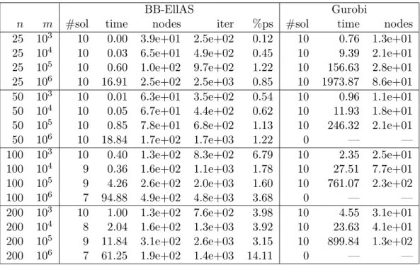
Table 1: Comparison on random binary instances.
BB-EllAS
Gurobi
n
m
#sol
time
nodes
iter
%ps
#sol
time
nodes
25
10
310
0.00
3.9e+01
2.5e+02
0.12
10
0.76
1.3e+01
25
10
410
0.03
6.5e+01
4.9e+02
0.45
10
9.39
2.1e+01
25
10
510
0.60
1.0e+02
9.7e+02
1.22
10
156.63
2.8e+01
25
10
610
16.91
2.5e+02
2.5e+03
0.85
10
1973.87
8.6e+01
50
10
310
0.01
6.3e+01
3.5e+02
0.54
10
0.96
1.1e+01
50
10
410
0.05
6.7e+01
4.4e+02
0.62
10
11.93
1.8e+01
50
10
510
0.85
7.8e+01
6.8e+02
1.13
10
246.32
2.1e+01
50
10
610
18.84
1.7e+02
1.7e+03
1.22
0
—
—
100
10
310
0.40
1.3e+02
8.3e+02
6.79
10
2.35
2.5e+01
100
10
49
0.36
1.6e+02
1.1e+03
1.78
10
27.51
7.7e+01
100
10
59
4.26
2.6e+02
2.0e+03
1.60
10
761.07
2.3e+02
100
10
67
94.88
4.9e+02
4.8e+03
3.68
0
—
—
200
10
310
1.00
1.3e+02
7.6e+02
3.98
10
4.55
3.1e+01
200
10
48
2.04
1.6e+02
1.3e+03
3.92
10
23.63
4.1e+01
200
10
59
11.84
3.1e+02
2.6e+03
3.15
10
899.84
1.3e+02
200
10
67
61.25
1.9e+02
1.4e+03
14.11
0
—
—
7.1
Random Instances
For a first comparison, we consider instances of Problem (P) where the objective function vectorc∈Rn
and the positive definite matrix Q ∈ Rn×n are randomly generated as described above. The set P is
explicitely given as{x∈Rn |Ax≤b}, whereA∈Rm×n andb∈Rmare also randomly generated: the
entries ofAwere chosen uniformly at random from the integers in the range [0,10] andb was defined by
bi =⌊12Pnj=1aij⌋, i = 1, . . . , m. Altogether, we generated 160 different problem instances for (P): for
each combination ofn∈ {25,50,100,200}andm∈ {103,104,105,106
}, we generated 10 instances. Since the setP is explicitely given here, the linear constraints are separated by enumeration inBB-EllAS. More precisely, at Step 8 of Algorithm 3, we pick the linear constraint most violated by x(k). We report our
results in Table 1.
From the results in Table 1, note that the average number of branch-and-bound nodes enumerated byBB-EllASis generally larger than the number of nodes needed by Gurobi, but always by less than a factor of 10 on average. However, in terms of running times,BB-EllASoutperforms Gurobi on all instance types except for the larger instances with a medium number of constraints, i.e., forn∈ {100,200}and
m∈ {104,105
}. On all other instance classes,BB-EllAS either solves significantly more instances than Gurobi within the time limit or has a faster running time by many orders of magnitude. This in confirmed by the performance profiles presented in Figure 1. The low number of iterations performed byEllASper node (less than 10 on average) highlights the benefits of using warmstarts.
7.2
Shortest Path Problem
Given a directed graphG= (V, E), whereV is the set of vertices and E is the set of edges, and weights associated with each edge, the Shortest Path problem is the problem of finding a path between two vertices s andt such that the sum of the weights of its constituent edges is minimized. Our approach
2 4 6 8 10 0 0.2 0.4 0.6 0.8 1 101 102 103
Robust Random Binary Instances
Gurobi BB-EllAS
Figure 1: Performance profile with respect to running times for random binary instances.
uses the following flow based formulation of the Robust Shortest Path problem: min c⊤x+p x⊤Qx s.t. P e∈δ+(i)xe−Pe∈δ−(i)xe = 0 ∀i∈V \ {s, t} P e∈δ+(s)xe−Pe∈δ−(s)xe = 1 P e∈δ+(t)xe−Pe∈δ−(t)xe = −1 x ∈ {0,1}E (6)
In our test set, we produced squared grid graphs with rrows and columns, where all edges point from left to right and from top to bottom. In this way, we produced graphs with |V| = r2 vertices and
|E|= 2r2−2redges. In the IP model (6), we thus haven:= 2r2−2rvariables and m:=|E|+ 2|V|=
4r2−2r many inequalities, taking into account also the box constraintsx
e∈[0,1] for e∈E. Since this
number is polynomial in n, we can separate them by enumeration within EllAS, whereas we can pass the formulation (6) to Gurobi directly. Concerning the objective function of (6), we set all expected lenghtsci to 1 and built the positive definite matrixQas described above. Altogether, we generated 100
different problem instances for (6): for eachr∈ {5, . . . ,14}we generated 10 instances.
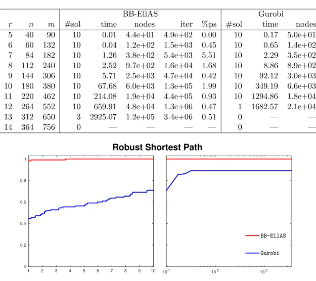
In Table 2, we report the comparison between BB-EllAS and the MISOCP solver of Gurobi. The average number of branch-and-bound nodes needed in BB-EllAS is in the same order of magnitude of that needed by Gurobi. However,EllASis able to process the nodes very quickly, leading to a branch-and-bound scheme that outperforms Gurobi in terms of computational time. Note also that for graphs withr = 13, Gurobi does not solve any instance within one hour CPU time, whileBB-EllASis able to solve 3 of them. Both solvers fail for instances withr≥14. See Figure 2 for the performance profiles.
7.3
Assigment Problem
Given an undirected, bipartite and weighted graph G = (V, E) with bipartition V = V1 ∪V2, the
Assignment problem consists in finding a one-to-one assignment from the nodes inV1to the nodes inV2
such that the sum of the weights of the edges used for the assignment is minimized. In other words, we search for a minimum-weight perfect matching in the bipartite graphG. Our approach uses the following
Table 2: Comparison on robust shortest path instances.
BB-EllAS
Gurobi
r
n
m
#sol
time
nodes
iter
%ps
#sol
time
nodes
5
40
90
10
0.01
4.4e+01
4.9e+02
0.00
10
0.17
5.0e+01
6
60
132
10
0.04
1.2e+02
1.5e+03
0.45
10
0.65
1.4e+02
7
84
182
10
1.26
3.8e+02
5.4e+03
5.51
10
2.29
3.5e+02
8
112
240
10
2.52
9.7e+02
1.6e+04
1.68
10
8.86
8.9e+02
9
144
306
10
5.71
2.5e+03
4.7e+04
0.42
10
92.12
3.0e+03
10
180
380
10
67.68
6.0e+03
1.3e+05
1.99
10
349.19
6.6e+03
11
220
462
10
214.08
1.9e+04
4.4e+05
0.93
10
1294.86
1.8e+04
12
264
552
10
659.91
4.8e+04
1.3e+06
0.47
1
1682.57
2.1e+04
13
312
650
3
2925.07
1.2e+05
3.4e+06
0.51
0
—
—
14
364
756
0
—
—
—
—
0
—
—
1 2 3 4 5 6 7 8 9 10 0 0.2 0.4 0.6 0.8 1 101 102 103Robust Shortest Path
Gurobi BB-EllAS
Figure 2: Performance profile with respect to running times for shortest path instances.
standard formulation of the Assignment problem: min c⊤x+p
x⊤Qx s.t. P
e∈δ(i)xe = 1 ∀i∈V
x ∈ {0,1}E
We consider complete bipartite graphs, so that the number of variables is n = 1 4|V|
2. The number of
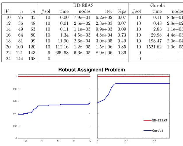
constraints includingx≥0 ism=|V|+n. Note that in the bipartite case the above formulation yields a complete description of conv(P∩Zn), which is not true in the case of general graphs. In our instances, we use expected weights 1 again, while the non-linear part of the objective function is generated as before. Altogether, we generated 80 different problem instances: for each|V| ∈ {10,12, . . . ,24}we generated 10 different instances. Results are presented in Table 3 and Figure 3. The general picture is very similar to the one for the Shortest Path problem.
Table 3: Comparison on robust assignment instances.
BB-EllAS
Gurobi
|
V
|
n
m
#sol
time
nodes
iter
%ps
#sol
time
nodes
10
25
35
10
0.00
7.9e+01
6.2e+02
0.07
10
0.11
8.3e+01
12
36
48
10
0.01
2.6e+02
2.3e+03
0.07
10
0.48
2.8e+02
14
49
63
10
0.11
1.1e+03
9.9e+03
0.09
10
2.83
1.1e+03
16
64
80
10
1.34
4.5e+03
4.8e+04
0.73
10
29.98
4.4e+03
18
81
99
10
11.90
2.6e+04
3.0e+05
0.49
10
198.47
2.0e+04
20
100
120
10
112.16
1.2e+05
1.5e+06
0.85
10
1521.62
1.0e+05
22
121
143
9
669.68
6.6e+05
8.9e+06
0.36
0
—
—
24
144
168
0
—
—
—
—
0
—
—
2 4 6 8 10 0 0.2 0.4 0.6 0.8 1 101 102 103Robust Assigment Problem
Gurobi BB-EllAS
Figure 3: Performance profile with respect to running times for assignment instances.
7.4
Spanning Tree Problem
Given an undirected weighted graph G = (V, E), a minimum spanning tree is a subset of edges that connects all vertices, without any cycles and with the minimum total edge weight. Our approach uses the following formulation of the Robust Spanning Tree problem:
min c⊤x+p x⊤Qx s.t. P e∈Exe = |V| −1 P e⊆Xxe ≤ |X| −1 ∀∅ 6=X⊆V x ∈ {0,1}E (7)
In the above model, the number of constraints, taking into account also the non-negativity constraints, is m = 2|V|+n. Since this number is exponential, we also have to use a separation algorithm for Gurobi. For bothBB-EllASand Gurobi, we essentially use the same simple implementation based on the Ford-Fulkerson algorithm.
For our experiments, we considered both complete graphs and grid graphs, the latter being produced as for the Shortest Path Problem. In both cases, expected edge weights are set to 1 again, while we
Table 4: Comparison on robust minimum spanning tree instances (complete graphs).
BB-EllAS
Gurobi
|
V
|
n
m
#sol
time
nodes
iter
%ps
#sol
time
nodes
10
45
1,069
10
2.93
1.4e+04
9.6e+04
1.35
10
78.59
1.6e+04
11
55
2,103
10
11.92
5.7e+04
4.3e+05
0.16
10
794.29
7.0e+04
12
66
4,162
10
120.84
4.4e+05
3.7e+06
0.06
1
2652.38
1.4e+05
13
78
8,270
10
1060.63
2.7e+06
2.4e+07
0.12
0
—
—
14
91
16,475
0
—
—
—
—
0
—
—
Table 5: Comparison on robust minimum spanning tree instances (grid graphs).
BB-EllAS
Gurobi
r
n
m
#sol
time
nodes
iter
%ps
#sol
time
nodes
5
40
3.4e+07
10
0.50
1.0e+03
8.7e+03
0.10
10
61.35
7.3e+03
6
60
6.9e+10
10
18.64
1.1e+04
1.2e+05
0.67
8
1805.72
9.2e+04
7
84
5.6e+14
9
1038.24
2.3e+05
3.3e+06
0.38
0
—
—
8
112
1.8e+19
0
—
—
—
—
0
—
—
built the positive definite matrixQ as above. Altogether, we generated 90 different problem instances: for each|V| ∈ {10, . . . ,14} we generated 10 different complete instances, while for each r∈ {5, . . . ,8} we generated 10 different grid instances. As shown in Tables 4 and 5,BB-EllASclearly outperforms the MISOCP solver of Gurobi on all the instances considered. For the performance profiles, see Figure 4.
2 4 6 8 10 0 0.2 0.4 0.6 0.8 1 101 102 103
Robust Minimum Spanning Tree
Gurobi BB-EllAS
Figure 4: Performance profile with respect to running times for spanning tree instances.
7.5
Traveling Salesman Problem
Given an undirected, complete and weighted graphG= (V, E), the Traveling Salesman problem consists in finding a path starting and ending at a given vertexv∈V such that all the vertices in the graph are
Table 6: Comparison on robust traveling salesman instances.
BB-EllAS
Gurobi
|
V
|
n
m
#sol
time
nodes
iter
%ps
#sol
time
nodes
10
45
1,157
10
0.70
3.5e+03
2.5e+04
1.73
10
15.50
3.3e+03
11
55
2,211
10
2.37
1.6e+04
1.3e+05
0.18
10
69.96
1.2e+04
12
66
4,292
10
17.59
9.6e+04
8.2e+05
0.05
10
637.47
7.1e+04
13
78
8,424
10
150.00
5.4e+05
4.8e+06
0.14
3
2324.42
2.3e+05
14
91
16,655
10
1087.76
2.5e+06
2.4e+07
0.25
0
—
—
15
105
33,081
1
2966.10
6.2e+06
6.0e+07
0.06
0
—
—
16
120
65,894
0
—
—
—
—
0
—
—
visited exactly once and the sum of the weights of its constituent edges is minimized. Our approach uses the following formulation of the Traveling Salesman problem:
min c⊤x+p x⊤Qx s.t. P e∈δ(i)xe = 2 ∀i∈V P e∈δ(X)xe ≥ 2 ∀∅ 6=X (V x ∈ {0,1}E (8)
Again, we consider complete graphs. The number of constraints including the bounds x ∈ [0,1]E is
m= 2|V|+ 3n−2 and hence again exponential. For both BB-EllASand Gurobi, we basically use the same separation algorithm as for the Spanning Tree problem; see Section 7.4. Instances are identical to those generated for the Spanning Tree problem, but we can consider slightly larger graphs, namely graphs with|V| ∈ {10, . . . ,16}. See Table 6 and Figure 5 for the results.
1 2 3 4 5 6 7 8 9 10 0 0.2 0.4 0.6 0.8 1 101 102 103
Robust Traveling Salesman Problem
Gurobi BB-EllAS
8
Conclusions
We presented a new branch-and-bound algorithm for robust combinatorial optimization problems under ellipsoidal uncertainty. We assume that the set of feasible solutions is given by a separation algorithm that decides whether a given point belongs to the convex hull of the feasible set or not, and, in the negative case, provides a valid but violated inequality. The branch-and-bound algorithm is based on the use of an active set method for the computation of dual bounds. Dealing with the Lagrangian dual of the continuous relaxation has the advantage of allowing an early pruning of the node. The closed form solution of the active set subproblems, the smart update of pseudo-inverse matrices, as well as the possibility of using warmstarts, leads to an algorithm that clearly outperforms the mixed-integer SOCP solver of Gurobi on the problem instances considered, including the robust counterpart of the shortest path and the traveling salesman problem.
9
Acknowledgments
The first author acknowledges support within the project “Mixed-Integer Non Linear Optimisation: Al-gorithms and Applications”, which has received funding from the Europeans Union’s EU Framework Programme for Research and Innovation Horizon 2020 under the Marie Sk lodowska-Curie Actions Grant Agreement No 764759. The second author acknowledges support within the project “Nonlinear Ap-proaches for the Solution of Hard Optimization Problems with Integer Variables”(No RP11715C7D8537BA) which has received funding from Sapienza, University of Rome.
References
[1] MOSEK ApS. The MOSEK optimization toolbox for MATLAB manual. Version 8.0.0.81, 2017. [2] A. Ben-Tal and A. Nemirovski. Robust convex optimization. Math. Oper. Res., 23(4):769–805, 1998. [3] A. Ben-Tal and A. Nemirovski. Robust solutions of uncertain linear programs. Oper. Res. Lett.,
25:1–13, 1999.
[4] A. Ben-Tal and A. Nemirovski. Lectures on Modern Convex Optimization. SIAM, Philadelphia., 2001.
[5] C. Buchheim, M. De Santis, S. Lucidi, F. Rinaldi, and L. Trieu. A Feasible Active Set Method with Reoptimization for Convex Quadratic Mixed-Integer Programming. SIAM Journal on Optimimiza-tion, 26(3):1695–1714, 2016.
[6] C. Buchheim, M. De Santis, F. Rinaldi, and L. Trieu. A Frank-Wolfe Based Branch-and-Bound Algorithm for Mean-Risk Optimization. Journal of Global Optimization, 70(3):625–644, 2018. [7] C. Buchheim and J. Kurtz. Robust combinatorial optimization under convex and discrete cost
uncertainty. Technical report, Optimization Online, 2017.
[8] E. Dolan and J.Mor´e. Benchmarking optimization software with performance profiles. Mathematical Programming, 91:201–213, 2002.
[9] Gurobi Optimization, Inc. Gurobi optimizer reference manual, 2016.
[10] P. Kouvelis and G. Yu. Robust Discrete Optimization and Its Applications. Springer, 1996. [11] C. D. Meyer. Matrix Analysis and Applied Linear Algebra. SIAM, Philadelphia, 2000.
[12] C. D. Meyer Jr. Generalized inversion of modified matrices.SIAM Journal on Applied Mathematics, 24(3):315–323, 1973.
[13] Hans D. Mittelmann. Mixed-integer SOCP Benchmark.http://plato.asu.edu/ftp/misocp.html (accessed March 1st, 2018; results from December 26th, 2017).
[14] Y. Nesterov and A. Nemirovski.Interior-point polynomial algorithms in convex programming. SIAM, Philadelphia, 1993.
[15] E. Nikolova. Approximation algorithms for offline risk-averse combinatorial optimization. Technical report, 2010.
[16] J. Nocedal and S. Wright. Numerical Optimization (Second Edition). Springer-Verlag, New York, 2006.
[17] J.F. Sturm. Using SeDuMi 1.02, a MATLAB toolbox for optimization over symmetric cones. Optimization Methods and Software, 11–12:625–653, 1999. Version 1.05 available from http://fewcal.kub.nl/sturm.