Solving Parity Games Using An
Automata-Based Algorithm
? ??Antonio Di Stasio1, Aniello Murano1, Giuseppe Perelli2? ? ?, Moshe Y. Vardi3 1
Universit`a di Napoli “Federico II”,2University of Oxford3Rice University
Abstract. Parity games are abstract infinite-round games that take an important role in formal verification. In the basic setting, these games are two-player, turn-based, and played under perfect information on directed graphs, whose nodes are labeled with priorities. The winner of a play is determined according to the parities (even or odd) of the minimal priority occurring infinitely often in that play. The problem of finding a winning strategy in parity games is known to be inUPTime∩CoUPTimeand deciding whether a polynomial time solution exists is a long-standing open question. In the last two decades, a variety of algorithms have been proposed. Many of them have been also implemented in a platform named PGSolver. This has enabled an empirical evaluation of these algorithms and a better understanding of their relative merits.
In this paper, we further contribute to this subject by implementing, for the first time, an algorithm based on alternating automata. More precisely, we consider an algorithm introduced by Kupferman and Vardi that solves a parity game by solving the emptiness problem of a corresponding alternating parity automaton. Our empirical evaluation demonstrates that this algorithm outperforms other algorithms when the game has a a small number of priorities relative to the size of the game. In many concrete applications, we do indeed end up with parity games where the number of priorities is relatively small. This makes the new algorithm quite useful in practice.
1
Introduction
Parity games[12,32] are abstract infinite-duration games that represent a powerful mathematical framework to address fundamental questions in computer science. They are intimately related to other infinite-round games, such asmean and
discounted payoff,stochastic, andmulti-agent games [3, 4, 6, 7].
In the basic setting, parity games are two-player, turn-based, played on directed graphs whose nodes are labeled with priorities (also called, colors) and
?An earlier version of the paper appeared in [11]. This version corrects a minor error in that earlier version. See Page 6.
?? Work supported by NSF grants CCF-1319459 and IIS-1527668, NSF Expeditions in Computing project ”ExCAPE: Expeditions in Computer Augmented Program Engineering”, BSF grant 9800096, ERC Advanced Investigator Grant 291528 (“Race”) at Oxford and GNCS 2016: Logica, Automi e Giochi per Sistemi Auto-adattivi. ? ? ?
players have perfect information about the adversary moves. The two players, Player 0 and Player 1, take turns moving a token along the edges of the graph starting from a designated initial node. Thus, a play induces an infinite path and Player 0 wins the play if the smallest priority visited infinitely often is even; otherwise, Player 1 wins the play. The problem of deciding if Player 1 has a winning strategy (i.e., can induce a winning play) in a given parity game is known
to be in UPTime∩CoUPTime[16]; whether a polynomial time solution exists
is a long-standing open question [31].
Several algorithms for solving parity games have been proposed in the last two decades, aiming to tighten the known complexity bounds for the problem, as well as come out with solutions that work well in practice. Among the latter, we recall the recursive algorithm (RE) proposed by Zielonka [32], the Jurdzi´nski’s small-progress measures algorithm [17] (SP), the strategy-improvement algorithm by Jurdzi´nski and V¨oge [29], the (subexponential) algorithm by Jurdzi´nki, Paterson and Zwick [18], and the big-step algorithm by Schewe [26]. These algorithms have been implemented in the platformPGSolver, and extensively investigated experimentally [13,14]. This study has also led to a few key optimizations, such as the decomposition into strongly connected components, the removal of self-cycles on nodes, and the application of a priority compression [2, 17]. Specifically, the latter allows to reduce a game to an equivalent game where the priorities are replaced in such a way they form a dense sequence of natural numbers, 1,2, . . . , d, for a minimal possibled. Table 1 summarizes the mentioned algorithms along with their known worst-case complexity, where the parametersn,e, andddenote the number of nodes, edges, and priorities, respectively (see [13, 14], for more).
Algorithm Computational Complexity
Recursive (RE) [32] O(e·nd)
Small Progress Measures (SP) [17] O(d·e·(nd)d2)
Strategy Improvement (SI) [29] O(2e·n·e)
Dominion Decomposition (DD) [18] O(n
√ n
) Big Step (BS) [26] O(e·n13d)
Table 1. Parity algorithms along with their computational complexities.
In formal system design [8,9,22,25], parity games arise as a natural evaluation machinery for the automatic synthesis and verification of distributed and reactive systems [1, 20, 28], as they allow to express liveness and safety properties in a very elegant and powerful way [23]. Specifically, in model-checking, one can check the correctness of a system with respect to a desired behavior, by checking whether a model of the system, that is, a Kripke structure, is correct with respect to a formal specification of its behavior, usually described in terms of a modal logic formula. In case the specification is given as aµ-calculus formula [19], the model checking question can be rephrased, in linear-time, as a parity game [12]. So, a parity game solver can be used as a model checker for aµ-calculus specification (and vice-versa), as well as for fragments such as CTL,CTL?, and the like.
In the automata-theoretic approach toµ-calculus model checking, under a linear-time translation, one can also reduce the verification problem to a question
about automata. More precisely, one can take the product of the model and an alternating tree automaton accepting all tree models of the specification. This product can be defined as an alternating word parity automaton over a singleton alphabet, and the system is correct with respect to the specification iff this automaton is nonempty [22]. It has been proved there that the nonemptiness problems for nondeterministic tree parity automata and alternating word parity automata over a singleton alphabet are equivalent and that their complexities coincide. For this reason, in the sequel we refer to these two kinds of automata just as parity automata. Hence, algorithms for the solution of the µ-calculus model checking problem, parity games, and the emptiness problem for parity automata can be interchangeably used to solve any of these problems, as they are linear-time equivalent. Several algorithms have been proposed in the literature to solve the non-emptiness problem of parity automata, but none of them has been ever implemented under the purpose of solving parity games.
In this paper, we study and implement an algorithm, which we call APT,
introduced by Kupferman and Vardi in [21], for solving parity games via emptiness checking of alternating parity automata, and evaluate its performance over the
PGSolverplatform. This algorithm has been sketched in [21], but not spelled
out in detail and without a correctness proof, two major gaps that we fill here. The core idea of theAPTalgorithm is an efficient translation to weak alternating automata [24]. These are a special case of B¨uchi automata in which the set of states is partitioned into partially ordered sets. Each set is classified as accepting or rejecting. The transition function is restricted so that the automaton either stays at the same set or moves to a smaller set in the partial order. Thus, each run of a weak automaton eventually gets trapped in some set in the partition. The special structure of weak automata is reflected in their attractive computational properties. In particular, the nonemptiness problem for weak automata can be solved in linear time [22], while the best known upper bound for the nonemptiness problem for B¨uchi automata is quadratic [5]. Given an alternating parity word automaton withnstates anddcolors, theAPTalgorithm checks the emptiness of an equivalent weak alternating word automaton with O(nd) states. The construction
goes through a sequence ofd intermediate automata. Each automaton in the
sequence refines the state space of its predecessor and has one less color to check in its parity condition. Since one can check in linear time the emptiness of such an automaton, we get anO(nd) overall complexity for the addressed problem.
APTdoes not construct the equivalent weak automaton directly, but applies the emptiness test directly, constructing the equivalent weak automaton on the fly.
We evaluated our implementation of theAPTalgorithm over several random game instances, comparing it withREandSPalgorithms. Our main finding is that when the number of the priority in a game is significantly smaller (specifically, logarithmically) than the number of nodes in the game graph, theAPTalgorithm significantly outperform the other algorithms. We take this as an important development since in many real applications of parity games we do get game instances where the number of priorities is indeed very small compared to the size of the game graph. For example, coming back to the automata-theoretic
approach toµ-calculus model checking [22], the translation usually results in a parity automaton (and thus in a parity game) with few priorities, but with a huge number of nodes. This is due to the fact that usually specification formulas are small, while the system is big. A similar phenomenon occurs in the application of parity games to reactive synthesis [28].
OutlineThe sequel of the paper is as follows. Section 2 gives preliminary concepts on parity games. Section 3 introduces extended parity games and describes theAPTalgorithm in detail, including a proof of correctness. Section 4 describes the implementation of theAPTalgorithm in the toolPGSolver. Section 5 contains the experimental results on runtime forAPTover random benchmarks. Finally, Section 6 gives some conclusions.
2
Preliminaries
In this section, we briefly recall some basic concepts regarding parity games. A
Parity Game (Pg, for short) is a tupleG,hPs,Ps,Mv,pi, where Ps and Ps
are two finite disjoint sets of nodes for Player 0 and Player 1, respectively, with Ps = Ps∪Ps, Mv ⊆Ps×Ps, is the left-total binary relation of moves, and
p: Ps→Nis the priority function1. Each player moves a token along nodes by
means of the relation Mv. By Mv(q),{q0 ∈Ps : (q, q0)∈Mv} we denote the set of nodes to which the token can be moved, starting from nodeq.
5 q 3 q q2 q1 5 q 2 q q2
Fig. 1. A parity game.
As a running example, consider the Pg
de-picted in Figure 1. The set of players’s nodes is Ps={q,q,q,q}and Ps={q,q,q}; we
use circles to denote nodes belonging to Player 0 and squares for those belonging to Player 1.Mv is described by arrows. Finally, the priority function pis given byp(q) = 1,p(q) =p(q) =p(q) =
2,p(q) = 3, andp(q) =p(q) = 5.
A play (resp., history) over G is an infinite (resp.,finite) sequenceπ=q·q·. . .∈Pth⊆Psω
(resp.,ρ=q·. . .·qn∈Hst⊆Ps∗) of nodes that
agree with Mv, i.e., (πi, πi+) ∈ Mv, for each natural number i ∈ N (resp.,
i∈[1, n−1]). In thePg in Figure 1, a possible play isπ=q·q·q·(q)ω,
while a possible history is given byρ=q·q·q·q.
For a given playπ=q·q·. . ., byp(π) =p(q)·p(q)·. . .∈Nω we denote
the associated priority sequence. As an example, the associated priority sequence toπis given byp(π) = 1·5·5·(2)ω.
For a given historyρ=q·. . .·qn, byfst(ρ),qand lst(ρ),qn we denote
the first and last node occurring inρ, respectively. For the example history, we have thatfst(ρ) =q andlst(ρ) =q. By Hst (resp.,Hst) we denote the set of
historiesρsuch that lst(ρ)∈Ps (resp.,lst(ρ)∈Ps). Moreover, by Inf(π) and
Inf(p(π)) we denote the set of nodes and priorities that occur infinitely often in
1
πandp(π), respectively. Finally, a playπis winning for Player 0 (resp., Player 1) if min(Inf(p(π))) is even (resp.,odd). In the running example, we have that Inf(π) ={q} andInf(p(π)) ={2} and so,πis winning for Player 0.
A Player 0 (resp.,Player 1) strategy is a function str : Hst →Ps (resp.,
str : Hst →Ps) such that, for all ρ ∈Hst (resp., ρ ∈ Hst), it holds that
(lst(ρ),str(ρ))∈Mv (resp., lst(ρ),str(ρ))∈Mv).
Given a nodeq, Player 0 and a Player 1 strategiesstr andstr, the play of
these two strategies, denoted byplay(q,str,str), is the only play πin the game
that starts inqand agrees with both Player 0 and Player 1 strategies,i.e., for alli∈N, ifπi ∈Ps, thenπi+=str(πi), andπi+=str(πi), otherwise.
A strategy str (resp., str) is memoryless if, for all ρ, ρ ∈ Hst (resp.,
ρ, ρ ∈ Hst), with lst(ρ) = lst(ρ), it holds that str(ρ) = str(ρ) (resp.,
str(ρ) =str(ρ)). Note that a memoryless strategy can be defined on the set
of nodes, instead of the set of histories. Thus we have that they are of the form str: Ps→Ps andstr: Ps→Ps.
We say that Player 0 (resp.,Player 1) wins the gameG from nodeqif there exists a Player 0 (resp., Player 1) strategy str (resp., str) such that, for all
Player 1 (resp.,Player 0) strategiesstr(resp.,str) it holds thatplay(q,str,str)
is winning for Player 0 (resp.,Player 1).
A nodeqiswinning for Player 0 (resp.,Player 1) if Player 0 (resp.,Player 1) wins the game fromq. By Win(G) (resp.,Win(G)) we denote the set of winning
nodes inGfor Player 0 (resp.,Player 1). Parity games enjoy determinacy, meaning that, for every nodeq, eitherq∈Win(G) orq∈Win(G) [12]. Moreover, it can
be proved that, if Player 0 (resp., Player 1) has a winning strategy from nodeq, then it has a memoryless winning strategy from the same node [32].
3
Extended Parity Games
In this section we recall theAPTalgorithm, introduced by Kupferman and Vardi in [21], to solve parity games via emptiness checking of parity automata. More important, we fill two major gaps from [21] which is to spell out in details the definition of the APTalgorithm as well as to give a correctness proof. TheAPT algorithm makes use of two special (incomparable) sets of nodes, denoted by V and A, and called set ofVisiting andAvoiding, respectively. Intuitively, a node is declared visiting for a player at the stage in which it is clear that, by reaching that node, he can surely induce a winning play and thus winning the game. Conversely, a node is declared avoiding for a player whenever it is clear that, by reaching that node, he is not able to induce any winning play and thus losing the game. The algorithm, in turns, tries to partition all nodes of the game into these two sets. The formal definition of the setsV andA follows.
AnExtended Parity Game, (Epg, for short) is a tuplehPs,Ps,V,A,Mv,pi
where Ps, Ps,Mv are as inPg. The subsets of nodes V,A⊆Ps = Ps∪Psare
two disjoint sets ofVisiting andAvoiding nodes, respectively. Finally,p: Ps→N
The notions of histories and plays are equivalent to the ones given forPg. Moreover, as far as the definition of strategies is concerned, we say that a play πthat is in Ps·(Ps\(V∪A))∗·V·Psωis winning for Player 0, while a playπ that is in Ps·(Ps\(V∪A))∗·A·Psωis winning for Player 1. For a playπthat never hits either V or A, we say that it is winning for Player 0 iff it satisfies the parity condition,i.e., min(Inf(p(π))) is even, otherwise it is winning for Player 1. Clearly, Pgs are special cases of Epgs in which V = A = ∅. Conversely, one can transform an Epginto an equivalentPgwith the same winning set by simply replacing every outgoing edge with loop to every node in V∪A and then relabeling each node in V and A with an even and an odd number, respectively.
In order to describe how to solve Epgs, we introduce some notation. By
Fi = p−(i) we denote the set of all nodes labeled with i. Doing that, the
parity condition can be described as a finite sequenceα= F·. . .·Fk of sets,
which alternates from sets of nodes with even priorities to sets of nodes with odd priorities and the other way round, forming a partition of the set of nodes, ordered by the priority assigned by the parity function. We call the set of nodes Fi an even (resp., odd) parity set ifiis even (resp.,odd).
For a given set X⊆Ps, byforce0(X) ={q∈Ps: X∩Mv(q)6=∅} ∪ {q∈Ps
: X⊆Mv(q)}we denote the set of nodes from which Player 0 can force to move in the set X. Analogously, byforce1(X) ={q∈Ps: X∩Mv(q)6=∅} ∪ {q∈Ps:
X⊆Mv(q)}we denote the set of nodes from which Player 1 can force to move in the set X. For example, in thePgin Figure 1,force1({q}) ={q,q,q}.
We now introduce two functions that are co-inductively defined that will be used to compute the winning sets of Player 0 and Player 1, respectively.
For a givenEpgGwithαbeing the representation of its parity condition, V its visiting set, and A its avoiding set, we define the functions Win(α,V,A) and
Win(α,A,V). Informally, Win(α,V,A) computes the set of nodes from which
the player 0 has a strategy that avoids A and either force a visit in V or he wins the parity condition. The definition is symmetric for the function Win(α,A,V).
Formally, we define Win(α,V,A) and Win(α,A,V) as follows.
Ifα=εis the empty sequence, then
– Win(ε,V,A) =force0(V) and – Win(ε,A,V) =force1(A).
Otherwise, ifα= F·α0, for some set F, then
– Win(F·α0,V,A) =µY(Ps\Win(α0,A∪(F\Y),V∪(F∩Y)))2 and – Win(F·α0,A,V) =µY(Ps\Win(α0,V∪(F\Y),A∪(F∩Y))),
whereµis the least fixed-point operator3.
2
In [11] the set Winis mistakenly typed as Ps\µY(Win(α0,A∪(F\Y),V∪(F∩Y))). Here, we provide its correct formulation. Please, note that in the proof of [11, Theorem 1], the formula is correctly reported.
3 The unravelling of Win
and Winhas some analogies with the fixed-point formula introduced in [30] also used to solve parity games. Unlike our work, however, the formula presented there is just a translation of the Zielonka’s algorithm [32].
To better understand howAPTsolves a parity game we show a simple piece of execution on the example in Fig 1. It is easy to see that such parity game is won by Player 0 in all the possible starting nodes. Then, the fixpoint returns the entire set Ps. The parity condition is given by α= F1·F2·F3·F4·F5, where
F1 ={q}, F2={q,q,q}, F3 ={q}, F4=∅, F5 ={q,q}. The repeated
application of functions Win(α,V,A) and Win(α,A,V) returns:
Win(α,∅,∅) =µY1(Ps\µY2(Ps\µY3(Ps\µY4(Ps\µY5(Ps\force1(V6))))))
in which the sets Yi are the nested fixpoint of the formula, while the set V
is obtained by recursively applying the following:
– V1=∅, Vi+1= Ai∪(F
i\Yi), and – A1=∅, Ai+1= Vi∪(F
i∩Yi).
As a first step of the fixpoint computation, we have that Y1= Y2= Y3=
Y4 = Y5=∅. Then, by following the two iterations above for the example in Figure 1, we obtain that V={q,q,q,q}.
At this point we have thatforce1(V6) ={q,q,q,q} 6=∅= Y. This means
that the fixpoint for Y has not been reached yet. Then, we update the set Y with the new value and compute again V. This procedure is repeated up to the
point in whichforce1(V6) = Y, which means that the fixpoint for Y has been
reached. Then we iteratively proceed to compute Y= Ps\Y until a fixpoint
for Y is reached. Note that the sets Ai and Vi depends on the Yi and so they
need to be updated step by step. As soon as a fixpoint for Y is reached, the
algorithm returns the set Ps\Y. As a fundamental observation, note that, due
to the fact that the fixpoint operations are nested one to the next, updating the value of Yi implies that every Yj, withj > i, needs to be reset to the empty set.
We now prove the correctness of this procedure. Note that the algorithm is an adaptation of the one provided by Kupferman and Vardi in [21], for which a proof of correctness has never been shown.
Theorem 1. Let G=hPs,Ps,V,A,Mv,pibe an Epgwith αbeing the parity sequence condition. Then, the following properties hold.
1. Ifα=εthenWin(G) = Win(α,V,A) andWin(G) = Win(α,V,A); 2. Ifαstarts with an odd parity set, it holds thatWin(G) = Win(α,V,A); 3. Ifαstarts with an even parity set, it holds thatWin(G) = Win(α,V,A). Proof. The proof of Item 1 follows immediately by definition, asα=forces the two players to reach their respective winning sets in one step.
For Item 2 and 3, we need to find a partition of F into a winning set for Player 0 and a winning set for Player 1 such that the game is invariantw.r.t.the winning sets, once they are moved to visiting and avoiding, respectively. We proceed by mutual induction on the length of the sequenceα. As base case, assumeα= F and F to be an odd parity set. Then, first observe that Player 0 can win only by eventually hitting the set V, as the parity condition is made by only odd numbers.
We have that Win(F,V,A) =µY(Ps\Win(ε,A∪(F\Y),V∪(F∩(Y)))) =
µY(Ps\force1(A∪(F\Y))) that, by definition, computes the set from which
Player 1 cannot avoid a visit to V, hence the winning set for Player 0. In the case the set F is an even parity set the reasoning is symmetric.
As an inductive step, assume that Items 2 and 3 hold for sequencesαof length n, we prove that it holds also for sequences of the form F·αof lengthn+1. Suppose that F is a set of odd priority. Then, we have that, by induction hypothesis, the formula Win(α,A∪(F\Y),V∪(F∩Y)) computes the winning set for Player 1
for the game in which the nodes in F∩Y are visiting, while the nodes in F\Y are avoiding. Thus, its complement Ps\Win(α,A∪(F\Y),V∪(F∩Y)) returns the
winning set for Player 0 in the same game. Now, observe that, if a set Y0 is bigger than Y, then Ps\Win(α,A∪(F\Y0),V∪(F∩Y0)) is the winning set for Player 0 in
which some node in F\Y has been moved from avoiding to visiting. Thus we have that Ps\Win(α,A∪(F\Y),V∪(F∩Y))⊆Ps\Win(α,A∪(F\Y0),V∪(F∩Y0)).
Moreover, observe that, if a nodeq∈F∪A is winning for Player 0, then it can be avoided in all possible winning plays, and so it is winning also in the case qis only in F. It is not hard to see that, after the last iteration of the fixpoint operator, the two sets F\Y and F∩Y can be considered in avoiding and winning, respectively, in a way that the winning sets of the game are invariant under this update, which concludes the proof of Item 2.
Also in the inductive case, the reasoning for Item 3 is perfectly symmetric to the one for Item 2.
4
Implementation of
APT
in
PGSolver
fun win i G Ps α V A = i f(α6=) then W := Ps\( m i n f p (1−i) G Ps αA V ) ; e l s e W :=forcei(V) ; returnW; ; fun m i n f p i G Ps α V A = Y1 := ∅; Y2 := ∅; F := head [α] ; α0 := t a i l [α] ; V0 := V∪F ; A0 := A ; Y2 := win i G Ps α0 V0 A0 ; while( Y26= Y1) do Y1 := Y2 ; V0 := V∪(F∩Y1) ; A0 := A∪(F\Y 1) ; Y2 := win i G Ps α0 V0 A0 ; done return Y2; ;
Fig. 2.APT Algorithm
In this section we describe the
im-plementation of APT in the
well-known platform PGSolver
devel-oped in OCaml by Friedman and Lange [14], which collects the large majority of the algorithms intro-duced in the literature to solve parity games [15, 17, 18, 26, 27, 29, 32].
We briefly recall the main aspects of this platform. The graph data struc-ture is represented as a fixed length array of tuples. Every tuple has all information that a node needs, such as the owner player, the assigned pri-ority and the adjacency list of nodes. The platform implements a collection of tools to generate and solve parity games, as well as compare the per-formance of different algorithms. The
deploy and test a generic solution algorithm, but also to investigate the practical aspects of the different algorithms on the different classes of parity games. More-over,PGSolverimplements optimizations that can be applied to all algorithms in order to improve their performance. The most useful optimizations in practice are decomposition into strongly connected components, removal of self-cycles on nodes, and priority compression.
We have added toPGSolveran implementation of theAPTalgorithm
intro-duced in Section 3. Our procedure applies the fixpoint algorithm to compute the set of winning positions in the game by means of two principal functions that implement the two functions of the algorithm core processes, i.e., function forcei and the recursive function Wini(α, V, A). The pseudocode of the APT
al-gorithm implementation is reported in Figure 2. It takes six parameters: the Player (0 or 1), the game, the set of nodes, the conditionα, the set of visiting and avoiding. Moreover, we define the function min fpfor the calculation of the fixed point. The whole procedure makes use of Set and List data structures, which are available in the OCaml’s standard library, for the manipulation of the sets visiting and avoiding, and the accepting conditionα. The tool along with the implementation of theAPT algorithm is available for download from https://github.com/antoniodistasio/pgsolver-APT.
For the sake of clarity, we report that inPGSolverit is used the maximal priority to decide who wins a given parity game. Conversely, theAPTalgorithm uses the minimal priority. However, these two conditions are well known to be equivalent and, in order to compare instances of the same game on different implementations of parity games algorithms inPGSolver, we simply convert the game to the specific algorithm accordingly. For the conversion, we simply use a suitable permutation of the priorities.
5
Experiments
In this section, we report the experimental results on evaluating the performance
for theAPTalgorithm implemented inPGSolverover the random benchmarks
generated in the platform. We have compared the performance of the implemen-tation of APTwith those ofREand SP. We have chosen these two algorithms as they have been proved to be the best-performing in practice [14].
All tests have been run on an AMD Opteron 6308 @2.40GHz, with 224GB
of RAM and 128GB of swap running Ubuntu 14.04. We note thatAPThas been
executed without applying any optimization implemented inPGSolver[14], while SPandREare run with such optimizations. Applying these optimization on APT is a topic of further research.
We evaluated the performance of the three algorithms over a set of games that are randomly generated by PGSolver, in which it is possible to give the numbernof states and the numberkof priority as parameters. We have taken 20 different game instances for each set of parameters and used the average time among them returned by the tool. For each game, the generator works as follows. For each nodeqin the graph-game, the priorityp(q) is chosen uniformly between
0 andk−1, while its ownership is assigned to Player 0 with probability 1 2, and
to Player 1 with probability 12. Then, for each nodeq, a numberdfrom 1 tonis chosen uniformly andddistinct successors ofqare randomly selected.
5.1 Experimental results
2 Pr 3 Pr 5 Pr
n RE SP APT RE SP APT RE SP APT
2000 4.94 5.05 0.10 4.85 5.20 0.15 4.47 4.75 0.42 4000 31.91 32.92 0.17 31.63 31.74 0.22 31.13 32.02 0.82 6000 107.06 108.67 0.29 100.61 102.87 0.35 100.81 101.04 1.39 8000 229.70 239.83 0.44 242.24 253.16 0.5 228.48 245.24 2.73 10000 429.24 443.42 0.61 482.27 501.20 0.85 449.26 464.36 3.61 12000 772.60 773.76 0.87 797.07 808.96 0.98 762.89 782.53 6.81 14000 1185.81 1242.56 1.09 1227.34 1245.39 1.15 1256.32 1292.80 10.02
Table 2.Runtime executions with fixed priorities 2, 3 and 5
We ran two experiments. First, we tested games with 2, 3, and 5 priorities, where for each of them we measured runtime performance for different state-space sizes, ranging in{2000,4000,6000,8000,10000,12000,14000}. The results are in Table 2, in which the number of states is reported in column 1, the number of colors is reported in the macro-column 2, 3, and 5, each of them containing the runtime executions, expressed in seconds, for the three algorithms.
n Pr RE SP APT n= 2k 1024 10 1.25 1.25 8.58 2048 11 7.90 8.21 71.08 4096 12 52.29 52.32 1505.75 8192 13 359.29 372.16 abortT 16384 14 2605.04 2609.29abortT 32768 15 abortT abortT abortT
n=ek 21 3 0 0 0 55 4 0 0 0.02 149 5 0.01 0.01 0.08 404 6 0.14 0.14 0.19 1097 7 1.72 1.72 0.62 2981 8 24.71 24.46 7.88 8104 9 413.2.34 414.65 35.78 22027 10 abortT abortT 311.87 n= 10k 10 1 0 0 0 100 2 0 0 0 1000 3 1.3 1.3 0.04 10000 4 738.86 718.24 4.91 100000 5 abortMabortM 66.4
Table 3.Runtime executions with
n=ekandn= 2kandn= 10k
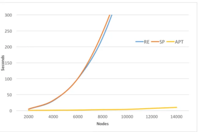
Second, we evaluated the algorithms on games with an exponential number of nodesw.r.t.the number of priorities. More precisely, we ran experiments for n= 2k, n=ek andn= 10k, wheren is the number of states andk is the number of priorities.
The experiment results are reported in Ta-ble 3. ByabortT, we denote that the execution
has been aborted due to time-out (greater of one hour), while byabortMwe denote that the
execution has been aborted due to mem-out. The first experiment shows that with a fixed number of priorities (2, 3, and 5) APT signifi-cantly outperforms the other algorithms, show-ing excellent runtime execution even on fairly large instances. For example, forn= 14000, the
running time for bothRE andSP is about 20
minutes, while forAPTit is less than a minute. The results of the exponential-scaling exper-iments, shown in Table 3, give more nuanced results. Here,APTis the best performing algo-rithm for n =ek andn = 10k. For example,
memout, while APTcompletes in just over one minute. That is, the efficiency of APTis notable also in terms of memory usage. At the sameAPTunderperforms
for n = 2k. Our conclusion is that APT has superior performance when the
number of priorities is logarithmic in the number of game-graph nodes, but the base of the logarithm has to be large enough. As we see experimentally, e is sufficiently large base, but 2 is not. This point deserve further study, which we leave to future work. In Figure 3 we just report graphically the benchmarks in the casen=ek. An interested reader can find more detailed experiment results
athttps://github.com/antoniodistasio/pgsolver-APT.
Fig. 3.Runtime executions withn=ek
6
Conclusion
TheAPTalgorithm, an automata-theoretic technique to solve parity games, has been designed two decades ago by Kupferman and Vardi [21], but never considered to be useful in practice [13]. In this paper, for the first time, we fill missing gaps and implement this algorithm. By means of benchmarks based on random games, we show that it is the best performing algorithm for solving parity games when the number of priorities is very smallw.r.t. the number of states. We believe that this is a significant result as several applications of parity games to formal verification and synthesis do yield games with a very small number of priorities. The specific setting of a small number of priorities opens up opportunities for specialized optimization technique, which we aim to investigate in future work. This is closely related to the issue of accelerated algorithms for three-color parity games [10]. We also plan to study why the performance of theAPTalgorithm is so sensitive to the relative number of priorities, as shown in Table 3.
References
1. B. Aminof, O. Kupferman, and A. Murano. Improved Model Checking of Hierar-chical Systems. Inf. Comput., 210:68–86, 2012.
2. A. Antonik, N. Charlton, and M. Huth. Polynomial-Time Under-Approximation of Winning Regions in Parity Games. ENTCS, 225:115–139, 2009.
3. D. Berwanger. Admissibility in Infinite Games. InSTACS’07, pages 188–199, 2007. 4. K. Chatterjee, L. Doyen, T. A. Henzinger, and J.-F. Raskin. Generalized
Mean-payoff and Energy Games. InFSTTCS’10, LIPIcs 8, pages 505–516, 2010. 5. K. Chatterjee and M. Henzinger. AnO(n2) Time Algorithm for Alternating B¨uchi
Games. InSODA’12, pages 1386–1399, 2012.
6. K. Chatterjee, T. A. Henzinger, and M. Jurdzinski. Mean-payoff parity games. In
LICS’05, pages 178–187, 2005.
7. K. Chatterjee, M. Jurdzinski, and T. A. Henzinger. Quantitative stochastic parity games. InSODA’04, pages 121–130, 2004.
8. E.M. Clarke and E.A. Emerson. Design and Synthesis of Synchronization Skeletons Using Branching-Time Temporal Logic. InLP’81, LNCS 131, pages 52–71, 1981. 9. E.M. Clarke, O. Grumberg, and D.A. Peled. Model Checking. 2002.
10. L. de Alfaro and M. Faella. An Accelerated Algorithm for 3-Color Parity Games with an Application to Timed Games. InCAV’07, LNCS 4590, pages 108–120, 2007. 11. A. Di Stasio, A. Murano, G. Perelli, and M. Vardi. Solving parity games using
an automata-based algorithm. InImplementation and Application of Automata -21st International Conference, CIAA 2016, Seoul, South Korea, July 19-22, 2016, Proceedings, pages 64–76, 2016.
12. E.A. Emerson and C. Jutla. Tree Automata, µ-Calculus and Determinacy. In
FOCS’91, pages 368–377, 1991.
13. O. Friedmann and M. Lange. The PGSolver collection of parity game solvers.
University of Munich, 2009.
14. O. Friedmann and M. Lange. Solving Parity Games in Practice. InATVA, LNCS 5799, pages 182–196, 2009.
15. K. Heljanko, M. Kein¨anen, M. Lange, and I. Niemel¨a. Solving Parity Games by a Reduction to SAT. J. Comput. Syst. Sci., 78(2):430–440, 2012.
16. M. Jurdzinski. Deciding the Winner in Parity Games is in UP∩co-Up.Inf. Process. Lett., 68(3):119–124, 1998.
17. M. Jurdzinski.Small Progress Measures for Solving Parity Games. InSTACS, pages 290–301, 2000.
18. M. Jurdzinski, M. Paterson, and U. Zwick. A Deterministic Subexponential Algo-rithm for Solving Parity Games. SIAM J. Comput., 38(4):1519–1532, 2008. 19. D. Kozen. Results on the Propositionalµ-Calculus. TCS, 27(3):333–354, 1983. 20. O. Kupferman, M. Vardi, and P. Wolper. Module Checking.164(2):322–344, 2001. 21. O. Kupferman and M. Y. Vardi. Weak Alternating Automata and Tree Automata
Emptiness. InSTOC, pages 224–233, 1998.
22. O. Kupferman, M.Y. Vardi, and P. Wolper. An Automata Theoretic Approach to Branching-Time Model Checking. Journal of the ACM, 47(2):312–360, 2000. 23. F. Mogavero, A. Murano, and L. Sorrentino. On Promptness in Parity Games. In
LPAR’13, LNCS 8312, pages 601–618, 2013.
24. D.E. Muller, A. Saoudi, and P.E. Schupp. Weak Alternating Automata Give a Simple Explanation of Why Most Temporal and Dynamic Logics are Decidable in Exponential Time. InLICS’88, pages 422–427, 1988.
25. J.P. Queille and J. Sifakis. Specification and Verification of Concurrent Programs in Cesar. In81, LNCS 137, pages 337–351, 1981.
26. S. Schewe. Solving Parity Games in Big Steps. InFSTTCS’07, LNCS 4855, pages 449–460, 2007.
27. S. Schewe. An Optimal Strategy Improvement Algorithm for Solving Parity and Payoff Games. InCSL’08, LNCS 5213, pages 369–384, 2008.
28. W. Thomas. Facets of Synthesis: Revisiting Church’s Problem. InFOSSACS’09, LNCS 5504, pages 1–14, 2009.
29. J. V¨oge and M. Jurdzinski. A Discrete Strategy Improvement Algorithm for Solving Parity Games. InCAV’00, LNCS 1855, pages 202–215, 2000.
30. I. Walukiewicz. Pushdown Processes: Games and Model Checking. In CAV’96, pages 62–74, 1996.
31. T. Wilke. Alternating Tree Automata, Parity Games, and Modal µ-Calculus.
Bulletin of the Belgian Mathematical Society Simon Stevin, 8(2):359, 2001. 32. W. Zielonka. Infinite Games on Finitely Coloured Graphs with Applications to