DePaul University
DePaul University
Via Sapientiae
Via Sapientiae
Technical Reports
College of Computing and Digital Media
9-2008
Global Verification and Analysis of Network Access Control
Global Verification and Analysis of Network Access Control
Configuration
Configuration
Ehab Al-Shaer
DePaul UniversityWill Marrero
DePaul UniversityAdel El-Atawy
DePaul UniversityKhalid ElBadawi
DePaul UniversityFollow this and additional works at: https://via.library.depaul.edu/tr Part of the Computer Engineering Commons
Recommended Citation
Recommended Citation
Al-Shaer, Ehab; Marrero, Will; El-Atawy, Adel; and ElBadawi, Khalid. (2008) Global Verification and Analysis of Network Access Control Configuration.
https://via.library.depaul.edu/tr/8
This Article is brought to you for free and open access by the College of Computing and Digital Media at Via Sapientiae. It has been accepted for inclusion in Technical Reports by an authorized administrator of Via Sapientiae. For more information, please contact digitalservices@depaul.edu.
Towards Global Verification and Analysis of
Network Access Control Configuration
Ehab Al-Shaer, Will Marrero, Adel El-Atawy and Khalid ElBadawi
School of Computing,DePaul University, Chicago, IL, USA
{ehab,wmarrero,aelatawy,badawi}@cs.depaul.edu Abstract
Network devices such as routers, firewalls, IPSec gateways, and NAT are configured using access control lists. However, recent studies and ISP surveys show that the management of access control configurations is a highly complex and error prone task [4]. Without automated global configuration management tools, unreachablility and insecurity problems due to the misconfiguration of network devices become an ever more likely.
In this report, we present a novel approach that models the global end-to-end behavior of access control devices in the network including routers, firewalls, NAT, IPSec gateways for unicast and multicast packets. Our model represents the network as a state machine where the packet header and location determine the state. The transitions in this model are determined by packet header information, packet location, and policy semantics for the devices being modeled. We encode the semantics of access control policies with Boolean functions using binary decision diagrams (BDDs). We extended computation tree logic (CTL) to provide more useful operators and then we use CTL and symbolic model checking to investigate all future and past states of this packet in the network and verify network reachability and security requirements. The model is implemented in a tool called ConfigChecker. We gave special consideration to ensure an efficient and scalable implementation. Our extensive evaluation study with various network and policy sizes shows that ConfigChecker has acceptable computation and space requirements with large number of nodes and configuration rules.
I. INTRODUCTION
Network traffic might pass through many different network devices from source to destination. Examples of these devices include routers, firewalls, NAT, and IPSec gateways. Each of these devices operates based on locally configured access control polices, which typically consist of filtering rules matched against incoming traffic to determine the appropriate action. If there is a match, the corresponding action of the matching rule is performed. Forwarding, discarding or encrypting traffic are examples of rule actions in routers, firewalls and IPSec policies respectively. Moreover, the policy action in the NAT devices involves replacing IP source and destination addresses of outgoing and incoming packets respectively. The rule matching semantics might differ from one device to another. For instance, firewalls use first-trigger sequential matching but longest-prefix matching is used for routing. Another example, in IPSec tunnels, actions of all matched rules are applied recursively on the matching traffic [17].
A typical enterprise network might include hundreds to thousands of access control devices, each containing hundreds or possibly thousands of rules. Although access control policies are configured locally in isolation from each other, they are logically composed to implement global end-to-end reachability and security requirements. Manual analysis of the interaction among the policies of the many devices in the network with different syntax and semantics is infeasible. The increasing complexity of managing access control configurations due to larger networks and longer policies makes configuration errors highly likely [4]. These misconfigurations can cause major network failures such as reachability problems, security violations, and network vulnerabilities. Recent studies have found that more than 62% of network failures today are due to network misconfiguration [4]. Moreover, a recent survey by Arbor Networks shows that managing access control is one of the most challenging issues faced by ISPs.
2 In the past few years, many researchers have attempted to address various challenges in network configuration management. In [1], [17], [29], different techniques are presented to identify configuration conflicts between firewall and IPSec devices. Approaches for analyzing routing configuration using static or formal analysis [10], [27], and on-line debugging [4] are proposed. Top-down configuration approaches have also been proposed [5], [25]. Our system, ConfigChecker, provides comprehensive end-to-end network configuration analysis engine to model all network access control devices (routers, firewalls, NAT, IPSec gateways) and offer a rich logic-based interface for network configuration analysis.
ConfigChecker models the entire network as a state machine, where each state is defined by the location and header information of packets in the network. We model the behavior of each access control device using binary decision diagrams (BDDs) [8]. This network abstraction allows the use of symbolic model checking techniques [9] to verify reachability and security properties written in CTL [11]. Unlike previous work, ConfigChecker considers techniques to obtain an expressive interface and scalable implementation. We extended CTL to provide additional operators that are particulary useful for verifying security properties. We also use efficient variable ordering in the BDD encoding to optimize BDD operations and space requirement. Thus, ConfigChecker can verify reachability, and identify security policy violations such as backdoors or broken tunnels due to, for example, errors or inconsistency between any two or more devices in the network.
The rest of this paper is organized as follows. We first describe our network model and abstraction in Section II. Section III presents the implementation of the system. We then present ConfigChecker application in configuration verification and analysis in Section IV. In Section V, we present our evaluation framework and results. The related work is presented in Section VI. We finally present our conclusion and future remarks in Section VII.
II. THEMODEL
We model the network as a giant finite state machine. The state of the network is determined by the packets in the network. The relevant information about a packet includes the packet header information (which is what determines what various devices in the network do with the packet) together with the packet’s current location. We begin with a simple model where we abstract away details about the packet payload and focus only on the data contained in packet headers. We then extend this model to include certain payload information that results from the encapsulation performed by IPSec devices.
A. Basic Model
In the basic model, the only information we need about the packet is the source and destination information contained in the IP header and the current location of the packet in the network. Therefore, we can encode the state of the network with the following characteristic function:
σ:IPs×ports×IPd×portd×loc → {true, false}
IPs the 32-bit source IP address
portsthe 16-bit source port number
IPd the 32-bit destination IP address
portdthe 16-bit destination port number
loc the 32-bit IP address of the device currently processing the packet
The functionσencodes the state of the network by evaluating to true whenever the parameters used as input to the function correspond to a packet that is in the network and false otherwise. If the network contains 5 different packets, then exactly five assignments to the parameters of the function σ will result in true. Note that because we abstract payload information, we cannot distinguish between 2 packets that are at the same device if they also have the same IP header information.
3 Each device in the network can then be modeled by describing how it changes a packet that is currently located at the device. For example, a firewall might remove the packet from the network or it might allow it to move on to the device on the other side of the firewall. A router might change the location of the packet but leave all the header information of the packet unchanged. A device performing network address translation might change the location of the packet as well as some of the IP header information. A hub might copy the same packet to multiple new locations. The behavior of each of these devices can be described by a list of rules. Each rule has a condition and an action. The rule condition can be described using a Boolean formula over the bits of the state (the parameters of the characteristic functionσ). If the packet at the device matches (satisfies) a rule condition, then the appropriate action is taken. As described above, the action could involve changing the packet location as well as changing IP header information. In all cases, however, the change can be described by a Boolean formula over the bits of the state. Sometimes the new values are constant (completely determined by the rule itself), and sometimes they may depend on the values of some of the bits in the current state. In either case, a transition relation can be constructed as a relation or characteristic function over two copies of the state bits. An assignment to the bits/variables in the transition relation yields true if the packet described by the first copy of the bits will be transformed into a packet described by the second copy of the bits when it is at the device in question. Some examples of how real devices can be encoded in this way should help to illustrate our technique. However, to keep the formulas simple, the examples will contain only 2 bits for the source IP, destination IP, and location IP, and 1 bit for the source port and destination port. Real examples are basically identical, but with larger fields. The formulas will use the following variables:
s1, d1, l1 The high order bit in the source IP address, the destination IP address, and the location IP address respectively. s0, d0, l0 The low order bit in the source IP address, the destination IP address, and the location IP address respectively. sp, dp The source port bit and the destination port bit respectively.
s0
0, s01, d00, . . . The meaning of these variables is identical to the unprimed versions above, except that these variables represent
the values of the bits in the next state.
Firewall: Assume a firewall with IP address of 1 has its outbound interface connected to a device with IP address 3. Furthermore, suppose it allows all traffic from IP address 2 to any destination as well as all traffic destined to port 1 on the device with IP address 3 coming from any source. All other traffic is blocked. Then all packets that satisfy the following formula will be forwarded to the outgoing interface:
(s1∧s0)∨(d1∧d0∧dp)
Furthermore, in the new state, the packet will look identical, except that it’s location will be IP address 3. Therefore, the restriction on the new state is:
^ i∈{0,1,p} (s0i⇔si)∧ ^ i∈{0,1,p} (d0i⇔di)∧l01∧l00
Finally, this transformation only occurs if the packet is currently at the firewall. In other words, the current location of the packet must be IP address 1:
l1∧l0
Therefore, transition relation for this particular firewall is the conjunction of the three conditions above. In general, the filtering policy of any firewall can be converted into a formula similar to the one in the example. It would have the form, if the current location is equal to this device, and the packet header information is such that the firewall accepts the packet, then the new location of the packet is the device connected to the outgoing interface, and no other packet information changes in the new
4 state. This formula encodes the fact that all packets accepted by the firewall get forwarded to the device connected to the outgoing interface, while there is no next state for the packet if it does not accepted by the firewall.
This construction assumes that we can encode a firewall’s filtering policy as a Boolean formula over the bits in the packet header information. A simple (but quite large) disjunction of all the minterms representing packets that are accepted demonstrates that this is theoretically possible. In practice, a list of filtering rules is used to configure the behavior of the firewall. This list of rules can be used to directly construct the formula as demonstrated in [17].
Router: Assume a router with IP address 2 sends all packets destined for IP addresses 1 and 0 to IP address 0 (next hop), while all other packets are sent to IP address 3 as a default gateway. The logic for the routing decisions is given by the following formula:
(d1∧l10 ∧l00)∨(d1∧l01∧l00)
Since no packet header information changes we also have the restriction ^ i∈{0,1,p} (s0i⇔si)∧ ^ i∈{0,1,p} (d0i⇔di)
Finally, this transformation only takes place when the packet is currently at the router; therefore, the following restriction must be satisfied as well:
l1∧l0
The transition relation for this particular router is the conjunction of the three conditions above.
NAT device: We model a device that performs network address translation the same way we model a router, except that this device might change the packet header information. For example, suppose a NAT device with IP address 2 is hiding a service on port 1 of a device with IP address 3 behind it and the NAT device is connected to device with IP address 1 in front of it. So any traffic from IP address 3 port 1 is sent to IP address 1, but the source information is changed to IP address 2 port 0. Additionally, any inbound traffic destination IP address 2 and port 0 is really intended for the hidden service, so it is forwarded to location 3, but its header information is changed so that the destination is now IP address 3 port 1. We will assume all other traffic is blocked. The restrictions on this device look like:
[s1∧s0∧sp∧l01∧l00 ∧s01∧s00∧s0p∧ ^ i∈{0,1,p} (d0 i⇔di)] _ [d1∧d0∧dp∧l10 ∧l00∧d01∧d00∧d0p∧ ^ i∈{0,1,p} (s0i ⇔si)]
Once again, this only happens if the packet is at the NAT device, so we must have the additional restriction:
l1∧l0
The transition relation for this NAT device is the conjunction of the two conditions above.
Multicast: There is nothing that restricts us to having at most one outgoing transition for a packet. For example, suppose router with IP address 1 sends traffic destined to IP address 0, to IP addresses 2 and 3 as next hops. This behavior can be modeled with the following formula:
5 Once again, no packet information changes, so we add the restriction:
^ i∈{0,1,p} (s0 i⇔si)∧ ^ i∈{0,1,p} (d0 i⇔di)
And we would also need the restriction that the packet is currently at the router which in this case means
l1∧l0
B. Extended Model
In order to model devices that perform encapsulation, we need to extend the state space so that the packet information includes not only the top level IP header information, but also the IP headers that appear in the payload of encapsulated packets. We do this by adding extra copies of the IP header fields (source IP, source port, destination IP, an destination port), one extra copy for each additional level of encapsulation that we want to allow in the model. Additionally, each copy will need a few extra bits to encode other information that affects IPSec behavior (such tunnel vs. transport and AH vs. ESP). We also need an extra “valid” bit for each copy that records whether or not a particular IP header copy is actually being used or not. This bit will only be on if the packet has been encapsulated. Note that none of the devices discussed so far make use of these extra copies. In the extended model we would need to add further restrictions to the transition relations for these devices that ensure that the values of these extra bits are not changed by these devices.
IPSec: Our model for an IPSec device is best explained by comparing it to our model of a firewall. If a packet is not protected, then the transformation behaves much like firewall. If the packet is protected, then in addition to the normal forwarding behavior, we also modify the header information. Encapsulation is modeled by “shifting” all IP header information one level/copy deeper and setting the next available “valid bit”. The new IP header information is then assigned to the outermost header copy which is the one that is used by all devices to make routing/filtering/transformation decisions. If a packet is decapsulated, then all header information is “shifted out” one position and the deepest “valid bit” is cleared. Note that this assumes that at least one valid bit was set. If there was not valid bit set, then the packet we are trying to decapsulate is actually not encapsulated so it should be dropped. Note that some IPSec devices have a recursive semantics in that after transforming the packet, the packet is basically fed back through the IPSec device again. We easily handle this case by setting the next location of a protected packet to be the address of the same IPSec device.
To present a simplified model for the IPSec device, we will need to add copies of all the IP header bits. The simplest case is where there is only one possible level of packet encapsulation so we only need one copy of the IP header bits. We will use a “hat” mark over variable names to indicate they represent the inner nested packet header. For example, the variable db1
0
represents the value of the high order bit in the destination IP address that has been encapsulated and now resides in the packet payload in the new state. This bit plays no role in the behavior of the packet unless it is later decapsulated so that it becomes part of the actual packer header again. Suppose a device with IP address 0, sends a packet to IP address 3. The first hop lands the packet at IP address 1 which protects the packet by encapsulating it and sending it to IP address 2, which is both the next hop and the endpoint of the tunnel. The encapsulation requires that we make use of the copies of the header bits. We will use
6 the variable v to indicate that the encapsulated bits are valid (in use). The formula for the protection of this traffic is:
l0∧l1 (1) ∧s0∧s1∧d0∧d1 (2) ∧v∧v0 (3) ∧ ^ i∈{0,1,p} (sb0 i⇔si)∧ ^ i∈{0,1,p} (db0 i⇔di) (4) ∧s0 0∧s01∧s0p↔sp∧d00∧d01∧d0p↔dp (5) ∧l0 0∧l01 (6)
Note that line (1) ensures that the packet is at the IPSec device in question while line (2) ensures that the packet header satisfies the protection condition (namely a packet from IP address 0 to IP address 3). Line (3) ensures that the encapsulated bits are not currently being used while requiring that they be marked as used in the next state. Line (4) specifies that the current IP header bits should be copied to the encapsulated bits. Line (5) specifies what the new IP header information should look like. The packet now looks like it originated at IP address 1 and is destined for IP address 2. Finally, line (6) specifies the next hop for the packet.
More logic would have to be included for how other packets should be treated. That logic will look very much like the firewall logic where some packets are allowed to move to the next hop without any modification, while other packets are simply dropped. Finally, the dual of the rule above would need to appear in the encoding for the IPSec device with IP address 2. Instead of copying bits from the header information to the encapsulation bits and turning on the valid bit, we would copy bits from the encapsulation bits to the IP header and turn off the valid bit.
C. Model Checking
We have described how to construct a transition relation for each device in the network. Each such transition relation describes a list of outgoing transitions for the device it models. The formulas are constructed with the requirement that the current location be equal to the device being modeled, so these transitions can only be taken when a packet is at the device. To get the transition relation for the entire network, we simply take the disjunction of the formulas for the individual devices. This matches our intuition since the current location of a packet will match at most the location of one of the devices in the network and so only its transitions will apply.
Recall that this global transition relation is a characteristic function for transitions in the model. If we substitute the values for a packet that is in the system into the current state variables of the transition relation, what we are left with is a formula describing what the possible next states of that packet look like. We have all the machinery to perform symbolic model checking. We use BDDs for all the formulas described above and we use standard model checking algorithms to explore the state space and compute states that satisfy various CTL properties as we describe in section IV.
Continuing with our small example, suppose we want to find all packets that could reach IP address 1 in a single step. What we want to find is the restriction on the packet in the current state such that the transition relation can get us to a next state in which the location is 1. To simplify the notation, we use~v=hs0, s1, sp, d0, d1, dp, l0, l1ito represent the tuple of variables
that determine the state in the model. If we let T(~v, ~v0)be the global transition relation (assuming no IPSec devices, so no
encapsulation bits are needed), then the following formula characterizes the packets that can reach location 1 in a single hop: ∃~v0[T(~v, ~v0)∧l00∧l01]
7 Recall thatl0
0 andl01 are variables in~v0.
The BuDDy BDD package provides all the required operations (including quantification). The resulting formula only has the current state variables free. If an assignment to the current state variables results in the formula evaluating to true, then a packet with that IP header information at that location will reach location 1 in a single hop. For a much more complete description of symbolic model checking, the reader is encouraged to see [9].
III. IMPLEMENTATION A. Data Modeling and Variable Asignment
As described in section II, a state in our model consists of the values of the various bits in a packet header, together with a location ID for each device. We use 104 bits to encode the basic packet header information (protocol, source IP/port, destination IP/port), 2 bits to indicate IPSec modes and 5 bits for IPSec parameters for a total 111 bits for the packet header. Recall that the extended model requires us to track the encapsulation/decapsulation of packets that is performed by IPSec devices. This requires storing the old packet header information so that it can be restored once the encapsulated packet reaches the end of a tunnel. Allowing nested tunnels will require an extra copy per tunnel. In other words, if we allow 4 nested tunnels, then we will need to have 5 replicas of the packet headers; 5 * 111 or 555 bits. Moreover, to keep track of which of those copies are actually being used we need a “valid bit” per copy (the outermost copy is always valid), so another 4 bits for 559 bits. We encode the location via a 32 bits for the IP address of the device for a total of 591 bits to encode the state. Also, the transition relation requires two copies of the state bits, one for the current state and one for the next state for a total of 1182 variables for the transition relation.
Of course it will be infeasible to explicitly model a system with such high number of variables. However, by keeping track of the states and the transition relation implicitly via formulas represented using BDDs, it is possible to perform analysis on a model so large. A BDD represents a formula as decision graph where the nodes in the graph are vertices and the edges coming out of a vertex represent the two possible Boolean assignments to that variable. Thus, a complete assignment to all variables corresponds to a path in the graph which ends in a value of true or false, which is the value of the formula when given that assignment.
For our implementation, we are using BuDDy which is a well known package that implements BDD operations and memory management. The package is implemented in C, with an added encapsulation for C++.
B. Variable Ordering
The size of this graph (the BDD) is extremely sensitive to the order in which the variables appear in the decision graph. We use the common interleaving heuristic which places the next state copy of a variable right next to the current state copy of the variable in the ordering. Furthermore, we try to keep variables that are related, close to each other. For this model, variables that belong to different copies of the same field are tightly related. When a tunnel is created, the current packet header copies are “pushed” one level deeper and a new packet header is created at the outer most level and the opposite when a tunnel terminates. For example, suppose a packet header consisted of three variables, x, y, and z. Also suppose we had 3 copies of the packet header to keep track of, so we now label the variables x0, y0, z0, x1, y1, . . . where xi corresponds to the value of the variable xin theith nested copy of header information. To keep the bits of the copies near each other, we use the ordering x0, x1, x2, y0, y1, y2, z0, z1, z2. If we add the next state variables as primed variables, the ordering becomes x0, x00, x1, x01, x2, x02, y0, y00, y1, y10, y2, y20, z0, z00, z1, z01, z2, z20.
8 C. Supported Devices and Configuration Files
The network is specified by a configuration file that lists the policy files for all included devices plus it includes general network parameters (e.g., size, generation date, comments, etc). Each policy file fully specifies a device behavior. In general, there is a brief meta-data section (address, default router, etc), and a policy section (routing rules, filtering policy, etc).
Currently, we implement the following devices:
• Routers: A routing policy is provided where each rule has a destination IP prefix and a next Hop. A device address
(loc), and a default router is specified in the router’s meta data as well. To satisfy the longest matching prefix criteria, we assume routing rules are sorted with respect to mask length.
• Firewalls: Filtering rules follow the 5-tuple standard syntax, and they are compiled following the rule of precedence for
the first-match. To support stateful inspection, an extra keyword (“state”) is added when a rule should affect the state table for reverse filtering. Each rule is preceded with the direction (in/out).
• IPsec Gateways:IP sec rules are specified similarly to firewall rules, with an addition of transformation mechanism (i.e.,
ESP/AH, tunnel/transport, and encryption algorithm/keyID)
• NAT:NAT devices can implement 4 modes: srcIP,srcIP+port, dstIP, dstIP+port. Each mode specifies what fields are to be
translated by the device. The NAT table is provided according to the specified mode in the firm of pairs (old and new values).
• Hubs:This is the only device that has the capability of sending a packet to more than one location. The device is provided
with next locations to which a packet will be propagated.
• Subnets: This device represents a set of hosts collectively. Its configuration file is very brief: the address, subnet mask,
and he default router. D. Query User Interface
After loading the configuration files (i.e., routing, ACL’s, NAT, etc), the user can input queries via a text based interface to the engine. Queries are written in a very similar fashion to that shown in Table I. Moreover, the user is given control on how the output can be shown, and what fields to list their satisfying assignments. For example, the following short query script contains two queries: the first will list (up to 10 entries), all next hop and destination IP pairs for router 1.2.3.4, and the second will use pre-computed query answers for further processing (showing only those next hops with a 2.*.*.* as location).
Q1 = EX (loc(1.2.3.4)) Q1 : ExtractField loc dip Q1 : ListBounded 10 loc dip Q2 = Q1 and loc(2.0.0.0,8) Q2 : list loc dip
First, the Query itself is defined using any of the defined Boolean operators and CTL functions over all packet header fields, and network locations. Then, the query can be further processed to remove unwanted fields (e.g., source port restrictions from a firewall policy). Afterwards, a listing of satisfying assignments of fields of interest can be displayed in human readable format (automatically detected based on field type).
To define a query, constraints over fields can be defined in the form off ld(value). For example,dIP(14.15.16.0,24)is an expression setting the most-significant 24 destination IP variables to the value given. Also, it is possible to define ranges in the same way (e.g., for ports). Moreover, inter-field equality can be enforced, and it takes the form f ld1(f ld2, bits), which indicates thatf ld1 andf ld2 should be equal in their specified most-significant bits.
9 assignment listing, and limited length listing. Also, further queries can be defined that includes previously defined queries in their expression.
E. Operation Implementation and Extending Standard CTL
In order to accommodate the variety of queries we need to perform against a network, we added a few non-standard operators to our CTL-Boolean operators. Below is a categorization of our currently supported operators, both standard and added ones (full implementation will be shown in Appendix ).
• Boolean Operators: The basic Boolean operators are evaluated in accordance with their standard definitions: and,or,
xor,imp, etc. Also, we accept writing these operators in common programming language syntax: &,|,−>,=>, etc.
• CTL (standard): CTL supports future temporal operators:EX,EF,AX,AF,AU,EU,AG,EG. However, to support
the nature of our network model (i.e., incomplete transition definition), we modified A∗ operators not to be satisfied at dead end states.
EX(f) :
(∃(T ∧next(f))
AF(f) :
return∀(EX(true)∧(T →next(f)))
This modification adds the constraintEX(true)to guarantee that dead-end states (sinks) are not included in the result.
• CTL (reverse time): Some queries are more intuitive defined in reverse time. We added the mirror of each standard
operator. The only difference is that the provided condition (f in the previous snippet) is applied to the transition relation without being shifted to the next state, and the result is shifted backward to current state variable afterwards. For example,
EX :
prev(∃(f∧T))
• CTL (bounded):Another extension is using bounded operators. These bounds are used during the fixed-point search. For
example AF n(f,3), searches for states that will be satisfying f within 3 transitions only.
• Network specific operators:A basic operation was added:length(s1, s2), which returns the minimum number of transitions
that can lead from the first to the second state. These states are commonly represented by locations:loc(x.x.x.x), or can be more specific and include protocol, or service: loc(x.x.x.x)∧dport(80). In the latter case, we can ask questions like what is the shortest distance between web traffic between this client and that server.
• Configuration operators: A few functions were added that can retrieve some of the provided requirements of the system.
For example,P connect(x, y)wherexandy, are restrictions on the source and destination IP respectively, returns true or false based on whether these two nodes should be connected or not from a requirement point of view. Also, T connect, asks the same question based on the topology and physical connectivity (multi-hop connectivity). If either parameter is left as true (or any partial assignment as sIP(1.2.0.0,16)), then the return will be all pairs that will evaluate to true. F. Random Topology and Configuration Generation (ConfGen) Tool
Objectives: The lack of a single tool that can generate a single configuration collection for topology, routing, and security settings necessitates that we introduce our tool that can incorporate all of them in a single customizable generation environment. A separate tool has been implemented for topology generation along with their routing and security settings. Security settings include firewall access lists, and IPsec settings. Also, NAT and multicast are supported. The output of this tool is a set of text files, one per device to specify the settings (i.e., IP address, default router, and interfaces), and the policy with which to operate.
10 Design and Implementation: Based on the required network depth and breadth, a mesh is created with a router at each cell. These routers are then interconnected based on the branching factor required. Some of the routers are converted into subnets, and a single upstream router is designated as the default gateway. However, several routers can route to the subnet according to the required subnet density, and distribution. The routing information will then be propagated between routers, until the root router (upper left corner) is reached.
Afterwards, some links will be intercepted via firewalls. From the upstream/downstream nodes, a list of valid IPs will be selected as well as some IPs outside the whole network range. Also, the netmask sizes in the firewall rules, and the protocol distribution is customizable.
Another step is adding extra feature devices like NAT, and IPSec. IPSec connections are created as pairs between IPSec devices. Currently, we can support tunneling, transport modes, as well as modifiers for ESP and AH.
Further details about the ConfGen tool will be provided in a separate document. How to Run: Both tools can be downloaded from the project home-page:
http://www.mnlab.cs.depaul.edu/projects/ConfigChecker
The tools are self explanatory, and include command line help for parameters. The ConfGen settings are supplied via a configuration file to specify the probabilities, and network properties to generate. ConfigChecker has very simple command line options which are the configuration path and the number of recursive levels to support (how many IPsec encapsulations the model should be capable of correctly decapsulate). The queries are given in a separate file in the same directory as the configurations and called query1.txt, query2.txt, etc. However, a single file can contain many queries, numbered Q1, Q2, etc. Query numbers can repeat across files, but not in the same file.
IV. AUTOMATEDCONFIGURATIONVERIFICATION ANDANALYSISUSINGCONFIGCHECKER
In this section, we will show two approaches to analyze network configurations: (1) verifying that the end-to-end reachability of the access control configuration is sound and complete, and (2) verifying number of end-to-end security properties to identify misconfiguration or undesired network behavior such as policy conflicts [1], [3], [17], policy violation and suboptimized config-uration. For this purpose, we developed ConfigChecker Query Interface (CI) based on CTL [11] to demonstrate the effectiveness of ConfigChecker in verifying the end-to-end network configurations globally and transparently. However, developing a high-level configuration language that hides CTL primitives and offers more usable interface is not the focus of this paper but part of our future work.
A. ConfigChecker Query Interface– Extending CTL
We consider a number of end-to-end properties that we might want to verify about a network. For each property, we describe how that property can be expressed in a computation tree logic (CTL) query which we would feed to our tool. Generally, a query is a Boolean expression that is being executed against a network configuration that has been loaded and compiled into a transition relation as shown in Section II. The Boolean expression can be defined over any of the packet header fields, and can include standard Boolean operations as well as CTL primitives. A complete and formal presentation of CTL is in [11].
CTL has a number of temporal operators that allow specifications that express future behavior. Because CTL can be used for non-deterministic models, these temporal operators can require that some future state exhibits a behavior (exists) or all future states exhibit a behavior (forall). Our models are typically deterministic; however we do use non-determinism to model the possibility of multiple routes and to model multicast. For example, intuitively a state satisfiesEX(loc= 140.192.1.1), if there is a next state in which the packet is at location 140.192.1.1. A state satisfies AX(loc= 140.192.1.1)if in all next states, the
11 packet is at location 140.192.1.1. If multiple routes or multicast were being modeled, AX(loc = 140.192.1.1) would insist that there is only one next hop.
Similarly, a state satisfies EF(loc= 140.192.1.1) if there is a path from this state along which eventually the location of the packet is 140.192.1.1. A state satisfies AF(loc= 140.192.1.1) if along all paths from this state, eventually the packet is 140.192.1.1. Again, AF(loc = 140.192.1.1) would be useful to check that if there are multiple routes, they all lead to the same destination.
Although model checking commonly searches states in future sense, we extend CTL to include operators to enable investi-gating states in the past. We will use a superscript−with each of the operators described above to denote the identical operator but considering paths going backwards in time. These extra operators will be useful for us because many security properties have the form “if A is true now, then B must have happened in the past”. For example, EX f talks about a predecessor state (or hop) while EXf talks about a successor state. The implementation detail of the past operators can be found in the Appendix.
To make the discussion that follows simpler, we will refer to entire fields such as source IP, destination port, current location IP, without breaking these down into their component bits. So the condition IPs = 103.23.91.4 is really shorthand for a conjunction of 32 expressions, each assigning a single bit in the IP address.
In the following sections, we describe applications of ConfigChecker by referring to the queries in Table I. These queries need specific values/addresses to be customized to a certain network (e.g., ip addresses of routers, port, etc). However, as part of CI, these queries can be used iteratively over the entire value range.
B. Reachability Verification
Routinize misconfiguration is not the only cause of reachability problems. Other access control configuration in the path like firewall, NAT or IPSec might interfere with routing and also cause unreachability problems. Thus global end-to-end access control analysis is required to verify reachability. In this section, we show how ConfigChecker can prove the end-to-end reachability soundness and completeness of the access control configuration including all different devices. Thus, we do not assume all physically connected nodes should be actually connected through configuration like the case in routing-only analysis [20]. However, the valid connectivity is determined based on the Connectivity Requirement Policy (CRP) which considers the authorization access and the physical topology. So let us assume that Pconnect(src, dest)as a characterization function for all sets of allowed flows from srctodest(IP and port numbers) that represents CRP. In case of full assignment (IP and port are fully specified), this function simply returnstrueif the traffic is allowed in CRP andfalseotherwise. In case of a partial assignment (i.e., src/dest are range of IPs and ports), it returns a boolean expression of all allowed flows. In other words, CRP states what should be allowed end-to-end. Thus flows that do not satisfy CRP will be denied.
For a basic reachability questions: Q1 in Table I shows whether the IP and port address (a1) can reach the IP and port address (a2). Moreover, if all types of traffic are allowed between the two hosts, the result will be the truevalue, otherwise it will be a boolean expression that represents only flows (services) that will reach the destination. Of course, we can use port numbers a long with IP to query a specific flow. We use loc in both side to restrict this query to unspoofed flows: routers send traffic with src=x wherexis not the address of th routers. By omitting the restriction of the source address field at both sides, we can check for the possibility of sending spoofed packets as well.
Definition 1.A configuration, C, issoundif, for all nodesuandw, all possible paths fromutoware subset of (or implies) authorized paths inPconnect(u, w). In other words, no nodeucan reach nodewusing Cif this is not allowed in CRP. Note that uandw can be defined based on IP and port. If the port is unspecified then it all possible ports are considered in the analysis. Q2in the Table I states formally this condition using CI.
12 TABLE I
EXAMPLE OF QUERIES THAT CAN BE USED INCONFIGCHECKER,WITH A BRIEF EXPLANATION OF EACH. Basic reachability
Q1: (src=a1 ∧ dest=a2 ∧ loc(a1))→AF(src=a1 ∧ dest=a2 ∧ loc(a2))
Given a starting location and a flow, does packets of this flow eventually reach the destination?
Reachability Soundness
Q2: [loc(a1) ∧ src(a1) ∧ dst(a2) ∧ EF(loc(a2))] → Pconnect(a1, a2)
If the src can reach the destination in configuration then it must be allowed in CRP.
Reachability Completeness
Q3: Pconnect(a1, a2) → [loc(a1) ∧ src(a1) ∧ dst(a2) → EF(loc(a2))]
if CRP allowsa1to reacha2, then there must a path in the configuration that eventually allows
a1to reacha2.
Discovering routing loops Q4: loc(a1) ∧ EX(EF(loc(a1))
Is there a node that can reacha1and for the same flow it is the next hop ofa1?
Shadow or Bogus routing entries
Q5: EX(true)∧ ¬EX(true) ∧ (loc(router1)∨loc(router2). . .)
Given all routers, does any have a decision for traffic will never reach it from its previous hop?
End-to-end integrity of single/nested or cascaded IPSec encrypted tunnel
Q6: (src=a1∧dest=a2∧loc(a1)∧IP Sec(encT)) → AU((IP Sec(encT)∨loc→ G), loc(a2))
If the traffic is encrypted in a tunnel from the src then it will appear decrypted only at the destination or at intermediate authorized gateways(G)that allow for cascaded tunnels. IfG=f alse, then there are no intermediate gateways and the traffic must travel through a single tunnel.
Comparing configuration for backdoors or broken flows after route changes
Q7a: Corg ,[¬multiroute∧src=a1∧dest=a2∧loc(a1)→AF(loc(a2)∧src=a1∧dest=a2)] Q7b: Cnew,[multiroute∧src=a1∧dest=a2∧loc(a1)→AF(loc(a2)∧src=a1∧dest=a2)] Q7: Backdoors:¬Corg∧ Cnew,Broken flows:¬Cnew∧ Corg
what is different in the new configuration as compared with the ordinary original one. Is there any backdoor?
Sub-Optimal routing
Q8: EX(loc(a1))∧AFn(loc(2), length(EX(loc(a1)), loc(a2))−T)
Given two routers, is it possible to reach the second in less steps than that provided by routing tables?
Spuriousness
Q9: (loc(a1) ∧ EX(true)) → EF(dest ⇔ loc)
From any node, if there is a next-hope (not default route) then there must be packet that will eventually reaches the destination.
Intermediate Sink nodes
Q10: EX (true)∧ ¬EX(true)∧ ¬(loc⇔dest)
Sink Nodes: What are the nodes and the associated traffic that have a previous state but not next state?
Definition 2.A configuration,C, iscompleteif for all nodesuandw,Pconnect(u, w)subset of (or implies) all possible paths from utow. Intuitively, if the CRP does not authorize uto reach wthen there is no allowed path (no routing or packets are discarded) in C fromutow.Q3in the Table I states formally this condition using CI.
If soundness or completeness condition fails, then the negation of the resulting expression will give us the states of all incorrect configurations that violate the access authorization or the physical topology 1. Assuming the number of misconfigurations is not largely excessive, we can then extract every misconfiguration scenario (including flow and location) by finding a satisfying assignment using bdd-satoperator in BDD [21] and then fix it.
The soundness condition enforces Loop-free property. However, it is sometimes useful to verify this property for specific device configuration [20]. Q4in the Table I shows the loop-free condition for a node. Using ConfigChecker,Q4in the Table I given a node/router is there any other routers that can eventually reach back this router and yet considered for the a same flow as a next hope for this router.
13 C. Discovering Security and Reachability Misconfiguration
In this section, we show more examples of ConfigChecker queries to discover specific misconfiguration such as security violations or suboptimized configuration. Although some of these conditions might also unsatisfy soundness and completeness condition, it is useful to search for specific misconfiguration for debugging and recovery.
Shadowing or bogus entries:It is useful to know if an access control node has a forward entry for a flow that will never reach it. This could occur if for example there is an upstream node in the path discards a flow that is or accepted by a downstream router or firewall respectively. Another reason of this condition is the creation of bogus routing entries (i.e., invalid next-hop) due to routing protocol bugs.Q5 in the Table I shows how to detect his misconfiguration.
IPSec Tunnel Integrity: Is my traffic encrypted all the way from source to destination? Are the intermediate gateways authorized ones? In addition to reachability, ConfigChecker can be used to verify that if a given configuration also satisfies specific security properties such end-to-end encryption. It has been numerously reported that due to misconfiguration in IPSec VPN configuration a traffic might be seen as plain text although it was encrypted and tunneled from source to destination [17], [28]. Q6 in Table I verifies this property for both single and cascaded tunnels. Thus, it is important to verify the encryption integrity from source to destination over single/nested or cascaded tunnels. Q7in Table I verifies that if a traffic is encrypted in a tunnel (encT) at the source it will stay encrypted over the same tunnel till the destination, assuming we set G= f alse
to disallow cascaded tunnels. However, ifG includes the list of authorized gateways, it verifies the same security property on cascaded tunnels.
Discovering backdoors and broken flows:It is necessary to guarantee that changes in routing configuration as a result of, for example, link failures will not violate security properties such as allowing access that was originally denied. Correct firewall deployment when multi-routing is used can be sometimes tricky.Q7in Table I checks if multiple paths between any two hosts exhibit different flow or security properties. We implement this by comparing the configuration of the longest-prefix route, Corg, with multi-route configuration,Cnew, (a disjunctive of all possible routes). It is important to note that the backdoors exist only if Cnew offers more accessability than Corg. The opposite means reachability problems due to broken flows. Otherwise, the access control configurations are consistent before and after the change/failure.
Sub-optimal routing : If any flow can reach its destination in a fewer number of hops by using a different next hop at a router, then this is a case of sub-optimality which can be expressed using stretch factor [20]. Router configuration should forward packets to the neighbor that is closest to the destination. Q8 in Table I compares the distance from all neighbors to the final destination. This query returns any route better than the current one. Changing the subtracted constant T allows for flexibility in setting the stretch factor. The operator AFn works likeAF, but it places a bound on how many steps can be taken before something is satisfied using the operator length that determines the length of the shortest path between two states. For example, a state satisfies AFn(loc = 140.192.1.1,8) if all paths starting from this state, the packet reaches location 140.192.1.1 in at most 8 hops. The operator lengthdetermines the length of the shortest path between two states. For example,length(loc= 140.192.1.∗, loc= 128.2.200.∗ computes the length of the shortest path from a host with network ID 140.192.1.* and a host with network ID 128.2.200.*.
Spuriousness: A spurious traffic is forwarded/accepted by some routers/firewalls but it will not eventually reach the final destination because for example it was dropped by a firewall [1]. Assuming that this traffic unreachablility is desired, then this
14 0 2000 4000 6000 8000 10000 12000 14000 0 500 1000 1500 2000 2500 3000 3500 4000 Memory (kB) # of network nodes Transition relation All BDDs
Fig. 1. Impact of network size on space requirements for a whole network.
0 0.5 1 1.5 2 2.5 3 3.5 4 0 500 1000 1500 2000 2500 3000 3500 4000
Memory per device (kB)
# of network nodes
Fig. 2. Impact of network size on space requirement per device.
0 500 1000 1500 2000 2500 3000 3500 4000 0 1 2 3 4 5 6 7 Memory (kB)
# of rules in network configuration (in millions)
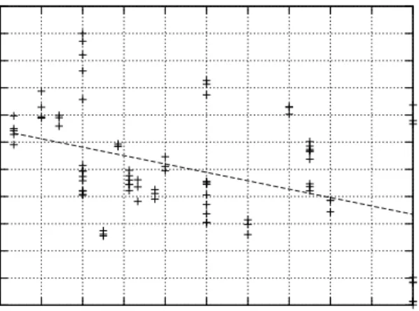
Fig. 3. Impact of network configuration size (in rule lines) on space complexity. 1.6 1.8 2 2.2 2.4 2.6 2.8 3 3.2 3.4 0% 20% 40% 60% 80% 100%
Memory per device (kB)
Subnets % of network size
Fig. 4. Impact of the percentage of subnets on network complexity/space.
traffic should have been blocked earlier in the path and thus called spurious. Spurious traffic is undesired by ISPs and enterprizes because it unnecessarily consumes bandwidth [1]. However, if this is not a desired property, then it flags out a bug or conflicts in access control configurations (routing and firewalls). This will also be detected in the soundness/completness conditions. Q9 in the Table I shows how to query for this misconfiguration using CI. Note thatQ9 is the property of uninterrupted flow, so the negation of this query result will be the spurious traffic. As before, we can find a satisfying assignment to extract the misconfiguration scenarios from the result of this query in order to fix them.
Sink nodes:In any specific network, some nodes should never be consumer nodes. In other words, there should be no traffic end its path at these nodes. Core routers are a typical example. If a packet got stuck at a router, it means that the routing table is missing information to route this packet. Moreover, firewalls and filtering devices in general (e.g., IDS) can be sink nodes according to their filtering policy. The query for this condition is shown in Q10 in Table I.
15 1.6 1.8 2 2.2 2.4 2.6 2.8 3 3.2 3.4 3.6 3.8 0 10 20 30 40 50 60 70 80 90 100
Memory per device (kB)
Branching Factor (% of network width)
Fig. 5. Impact of the branching factor (number of outgoing links) on the network complexity. 1.6 1.8 2 2.2 2.4 2.6 2.8 3 3.2 3.4 3.6 3.8 0.1 1 10
Memory per device (kB)
Ratio of depth to width of network
Fig. 6. Impact of the network’s aspect ratio (depth by width) on memory requirements. 0 20 40 60 80 100 120 0 50 100 150 200 0 20 40 60 80 100 120
Time to build (sec)
Memory (MB)
Number of added firewalls/IPSec Time Memory
Fig. 7. Time/memory required for three different networks (Each has 600 routers, 400 domains), while adding 0 to 200 firewalls. Firewall policies are all same size.
0 200 400 600 800 1000 1200 0 20 40 60 80 100 120 140 160 180 200 0 100 200 300 400 500 600
Time to build (sec)
Memory (MB)
Number of FW/IPSec rules (thousands) Time Memory
Fig. 8. Time/memory required for a network with 600 routers, 400 domains, and 50 firewalls. Number of rules in each FW ranged from 0 up to 4K rules.
V. EVALUATION
In this section, we provide space requirement and performance evaluation of the framework with respect to the memory and time requirements. We evaluated ConfigChecker using more than 85 networks. We focus our study on the time and space for building and running the model. We study the effect of several network configuration parameters: network size, connectivity (branching factor), number of subnets, number of configuration rules in the network, number of firewalls/IPSec devices and ACL rules. Due to the lack of tools to generate random network topologies with access control configuration that include, routing, firewalls and IPSec, we developed our own tool (ConfGen) to generate real and valid configurations based on random topologies (See project homepage for topologies and examples). Misconfigurations are manually injected for testing and evaluation purposes.
In the following discussion, network size is the overall number of nodes in the network including: routers, security devices, and domains. We used networks of size that ranged from 25 nodes up to 1200 nodes, with configuration sizes (routing tables, firewall/IPSec ACLs, etc) up to 4 million rules per network. It is worth mentioning that the execution time of all described queries is negligible.
16 0 10 20 30 40 50 2 3 4 5 6 7 8 9 0 2 4 6 8 10 12
Time to build (sec)
Memory required (MB)
Number of recursive levels (nested tunnels) max Time
min Time max Memory max Memory
Fig. 9. Time and memory required for two Networks of 1000 nodes each.
0 500 1000 1500 2000 2500 3000 3500 4000 4500 5000 1 2 3 4 5 6 7 8 9 BDD nodes
Number of recursive levels (nested tunnels) variables
Copier Push Pop
Fig. 10. Size requirements of copier expressions
1) Impact of Network Size: We first consider the impact of the network size (or number of nodes) on the space complexity of the overall model. Space requirements are measured by the number of BDD nodes used for the model. This includes variable information and links between nodes. Each node requires 20 bytes of memory in the used implementation (BuDDy [21]). In Figure 1, we can see that the space required to compile a network is linear in its size. For a thousand nodes, the space for the compiled model was less than 5MB which is very moderate considering the size. Our experiments also show that the memory requirement per devices stays in a constant range (2-5K) regardless of the network size. Our experiments also show that the memory requirement decreases when branching factor (the number of outgoing links per device) increases. This can be attributed to the BDD merging of common expressions due to the similarity of links encoding (bits) of a node.
2) Impact of the number of Subnets: As the percentage of subnets/domains defined in the network increases, the complexity of the model increases. Despite the fact that the number of network devices decreases in this case, we still see the dominant effect of routing information propagating in the network. Figure 4 shows the effect of subnet percentage on the space complexity for more than 20 networks of 1000 nodes each.
3) Impact of the configuration size: Configuration size measured in number of rules in routing and access control policies plays an obvious role in the overall network complexity. Figure 3 shows this relation clearly. However, we can see the growth stabilizing after a threshold where more configuration rules do not increase the space requirements. This behavior is due to two factors. First, the redundancy in routing rules that manifests itself when many routing rules are propagated without being effective on the network operations. Second, the capability of the BDD structure to merge expressions that are similar becomes more useful as policies increase in size.
4) Impact of Branching Factor: The number of outgoing links had a slight effect on the models used as shown in Figure 5. This can be attributed to the aggressive merging of common expressions of which the BDD structure is capable. Therefore, when a specific device has many outgoing links, only the links information is encoded. Moreover, the next devices all belong to the same layer which makes their addresses differ in a few bits enhancing the possibility of further optimization by the BDD. The branching factor is given as a percentage of upstream links used out of the possible routers in the next higher level. 5) Impact of Aspect Ratio: In Figure 6, we can see that the aspect ratio (i.e., Depth / Width of network) has no significant effect on the memory requirements per device in the model. However, one can notice that for smaller aspect ratio there is a higher variability in the memory requirements. This can be attributed to the wider range of the number of outgoing links resulting in more variability in the model and, in turn, a higher variability in complexity. In the figure, memory per device is
17 used instead of the overall memory requirements to eliminate the effect of network size.
6) Impact of adding filtering devices: Adding firewalls and IPSec devices is expected to increase the space and time complicity because more emphasis on new fields not used in routing. Figure 7 shows that as we add firewalls or IPSec devices (up to 200 added filtering devices to a network of 1000 nodes), both space and time appear to grow almost linearly. However, the effect of increasing the policy size while fixing the number of firewalls is more evident in terms of building time. This is due to the interaction between firewall rules (e.g., higher priority rules shadow the lower priority ones). Although this effect is usually quadratic, we reduce this effect in our implementation close to linear by exploiting the overlapping operations in BDDs. However, we can see in Figure 8 that the BDD operation is itself suffering slightly from the increased complexity of the overlapping rules, which was expected but yet still in reasonable range.
7) Impact of encapsulation levels: To support devices capable of packet encapsulation (i.e., IPSec), it is important to make sure the system is scalable in the number of encapsulation levels. In figure 9, we show that the time and space required are linear in the number of levels (IPSec nested tunnels) for both the minimum and the maximum cases . The two extreme network cases were chosen to have the same size (1000 nodes), but with varying branching density (30/device formaximum net and 10/device forminimum net).
8) Copying expressions complexity: As mentioned in Section II, we use expressions to be added to the transition relation of all devices to ensure packets are copied as is between transitions. These expressions are independent of the network structure, size, and specific information.
Clearly, as in Table II and in Figure 10, the memory requirements are quite moderate, and will not pose any significant overhead when analyzing and building real networks.
The following table shows the size (i.e., nodes in the BDD) used for each of the three expressions (“copy”, “push copy”, and “pop copy”) for different levels of encapsulation (e.g., levels=1 means no encapsulation supported, 2 a packet can be encapsulated once, etc).
TABLE II
VARIABLES AND OPERATIONS COST
Levels 1 2 3 4 5 6 7 8 9
Variables 282 500 718 936 1154 1372 1590 1808 2026 Copier 327 654 981 1308 1635 1962 2289 2616 2943 Push Copy 0 327 981 1635 2289 2943 3597 4251 4905 Pop Copy 0 327 654 981 1308 1635 1962 2289 2616
VI. RELATEDWORK
There have been significant research effort in the area of configuration verification and management in the past few years. We can classify the work in this area into two main approaches: top-down and bottom-up. The top-down approaches [5], [25] create clean-slate configurations based on high-level requirements. However, the bottom-up approaches [1], [17], [29] analyze the existing configuration to verify desired properties. We focus our discussion in the section on bottom-up approach as it is closer to our work in this paper.
There has been considerable work recently in detecting misconfiguration in routing and firewall. Many of these approaches are specific for BGP misconfiguration [4], [13], [15], [23]. However, other works attempt to create general models for analyzing network configuration [10], [27]. An approach for formulating and deriving of sufficient conditions of connectivity constraints is presented in [10]. The static analysis approach [27]is one of the most interesting work that is close to ConfigChecker. This work uses graph-based approach to model connectivity of network configuration and use set operations to perform static analysis. The transitive closure, as apposed to a fixed point in our approach, is computed. Thus, it seems that all possible paths
18 are computed explicitly. In addition, considering security devices and properties, providing a rich query interface based on our CTL extension, and utilizing BDDs optimization are major advantages of our work.
On the other hand, significant amount of work was done in the conflict analysis of firewalls configuration(e.g., [1], [17], [28], [29]). A BDD-based modeling and taxonomy of IPSec configuration conflicts was presented in [2], [17]. FIREMAN [29] uses BDD to show conflicts on Linux iptablesconfigurations. In [24] and [26], the authors developed a firewall analysis tool to perform customized queries on a set of filtering rules of a firewall. But no general model of network connections is used in this work.
Thus, in conclusion, although this body of work has a significant impact on the filed, it is either provide limited analysis due to restriction on specific network or application. Unlike the previous work, ConfigChecker offers a global configuration verification that is comprehensive, scalable and highly expressive.
In the field of distributed firewalls, current research mainly focuses on the management of distributed firewall policies. The first generation of global policy management technology is presented in [16], which proposes a global policy definition language along with algorithms for verifying the policy and generating filtering rules. In [7], the authors adopted a better approach by using a modular architecture that separates the security policy and the underlying network topology to allow for flexible modification of the network topology without the need to update the security policy. Similar work has been done in [18] with a procedural policy definition language, and in [22] with an object-oriented policy definition language. In terms of distributed firewall policy enforcement, a novel architecture is proposed in [19] where the authors suggest using a trust management system to enforce a centralized security policy at individual network endpoints based on access rights granted to users or hosts. We found that none of the published work in this area addressed the problem of discovering conflicts in distributed firewall environments.
A variety of approaches have been proposed in the area of policy conflict analysis. The most significant attempt for IPSec policy analysis is proposed in [14]. The technique simulates IPSec processing by tracking the protection applied on the traffic in every IPSec device. At any point in the simulation, if packet protection violates the security policy requirements, a policy conflict is reported. Although this approach can discover IPSec policy violations in a certain simulation scenario, there is no guarantee that it discovers every possible violation that may exist. In addition, the proposed technique only discovers IPSec conflicts resulting from incorrect tunnel overlapping, but do not address the other types of conflicts that we study in this research.
Top-down configuration management. Model finder [25] uses Alloy and SAT tools to create network configuration based on high-level constraints. FLIP [30] and Firmato [6] offer a high-level firewall languages and translation engine to create firewall rules based on user-level specification. Presto [12] provides a template-based approach to automate specific network management tasks. Firmato [6] is another firewall management toolkit, based on entity-relation model, that translate the user model into rules
VII. CONCLUSION ANDFUTUREWORK
Managing the configuration of network access control devices such as routers, NAT, firewalls, and IPSec gateways is extremely complex and error-prone. This paper presents a model checker approach based on Binary Decision Diagrams (BDDs) to create a unified model for network access control configuration regardless of devices function and matching semantic. We also extended CTL to provide an expressive query interface over this model for global end-to-end verification and ”what-if” analysis. The model is implemented in a tool calledConfigChecker. We demonstrate effectiveness and expressiveness power of ConfigChecker through the provability of soundness and completeness of the configuration reachability as well as crafting number of query
19 examples to detect (1) security violation such as backdoors or broken IPSec tunnels, (2) unreachability due to route failures or changes, and (3) sub-optimized configuration.
Our evaluation experiments using more than 85 networks of various configurations show that ConfigChecker requires less than 5KB per device or less than 5MB in total for 1200 nodes and millions of configuration rules. We also show that the time and space complexity grow linearly in a reasonable rate with the size of the network. The ConfigChecker implementation, query in-terface and the query examples stated in this paper are available in public from www.mnlab.cs.depaul.edu/projects/ConfigChecker.
In the future work, we plan to extend our model to include other devices like QoS, load balancer, IDS nodes. We also plan to create a high-level language that hides the CTL-like operators and make our tool highly usable by even regular users.
APPENDIX CTL ROUTINES
This is a trimmed version of the CTL class we implemented for ConfigChecker. It includes the standard, as well as some of the extended CTL operators. Also, some operators are added that are in the same class for convenience rather than formal correctness.
void CTL::Init(bdd TransRel) { T = TransRel;
Initialized = true;
NewVars = GetAllVarList(1) & GetVarList(fldLocationNew); OldVars = GetAllVarList(0) & GetVarList(fldLocation); EXtrue = EX(bddtrue); EX_true = EX_(bddtrue); }; bdd CTL::next(bdd f){ return bdd_replace(f,newOldPairs); }; bdd CTL::prev(bdd f){ return bdd_replace(f,oldNewPairs); }; bdd CTL::EX(bdd f){
if (!Initialized) throw CTLException(); return bdd_exist(next(f) & T,NewVars); };
bdd CTL::AX(bdd f){
if (!Initialized) throw CTLException();
return bdd_forall(EXtrue & bdd_imp(T,next(f)) ,NewVars); };
bdd CTL::EU(bdd f, bdd g){
if (!Initialized) throw CTLException(); bdd Y= bddfalse;
20 while (Y != oldY){ oldY = Y; Y = g | (f & EX(Y)); } return Y; };
bdd CTL::EUn(bdd f, bdd g, int bound){ if (!Initialized) throw CTLException(); bdd Y= bddfalse;
bdd oldY = bddtrue; int counting=0;
while ((Y != oldY) && (counting<bound)){ oldY = Y; Y = g | (f & EX(Y)); } return Y; }; bdd CTL::AU(bdd f, bdd g){
if (!Initialized) throw CTLException(); bdd Y= bddfalse; bdd oldY = bddtrue; while (Y != oldY){ oldY = Y; Y = g | (f & AX(Y)); } return Y; };
bdd CTL::AUn(bdd f, bdd g, int bound){ if (!Initialized) throw CTLException(); bdd Y= bddfalse;
bdd oldY = bddtrue; int counting=0;
while ((Y != oldY) && (counting<bound)){ oldY = Y; Y = g | (f & AX(Y)); } return Y; }; bdd CTL::EG(bdd f){
if (!Initialized) throw CTLException(); bdd Y = bddtrue;
bdd oldY = bddfalse; while (Y != oldY){
21 Y = f & EX(Y); }; return Y; }; bdd CTL::AG(bdd f){
if (!Initialized) throw CTLException(); bdd Y = bddtrue; bdd oldY = bddfalse; while (Y != oldY){ oldY = Y; Y = f & AX(Y); }; return Y; }; bdd CTL::EF(bdd f){
if (!Initialized) throw CTLException(); return EU(bddtrue, f);
};
bdd CTL::EFn(bdd f, int bound){
if (!Initialized) throw CTLException(); return EUn(bddtrue, f, bound);
};
bdd CTL::AF(bdd f){
if (!Initialized) throw CTLException(); return AU(bddtrue, f);
};
bdd CTL::AFn(bdd f, int bound){
if (!Initialized) throw CTLException(); return AUn(bddtrue, f, bound);
};
bdd CTL::EX_(bdd f){
return prev(bdd_exist(f & T, OldVars)); };
bdd CTL::AX_(bdd f){
return prev(bdd_forall( bdd_imp(T,f) ,OldVars)) & EX_(bddtrue); };
bdd CTL::EU_(bdd f, bdd g){
if (!Initialized) throw CTLException(); bdd Y= bddfalse;
22 bdd oldY = bddtrue; while (Y != oldY){ oldY = Y; Y = g | (f & EX_(Y)); } return Y; };
bdd CTL::EUn_(bdd f, bdd g, int bound){ if (!Initialized) throw CTLException(); bdd Y= bddfalse;
bdd oldY = bddtrue; int counting=0;
while ((Y != oldY) && (counting<bound)){ oldY = Y; Y = g | (f & EX_(Y)); } return Y; }; bdd CTL::AU_(bdd f, bdd g){
if (!Initialized) throw CTLException(); bdd Y= bddfalse; bdd oldY = bddtrue; while (Y != oldY){ oldY = Y; Y = g | (f & AX_(Y)); } return Y; };
bdd CTL::AUn_(bdd f, bdd g, int bound){ if (!Initialized) throw CTLException(); bdd Y= bddfalse;
bdd oldY = bddtrue; int counting=0;
while ((Y != oldY) && (counting<bound)){ oldY = Y; Y = g | (f & AX_(Y)); } return Y; }; bdd CTL::EG_(bdd f){
if (!Initialized) throw CTLException(); bdd Y = bddtrue;
bdd oldY = bddfalse; while (Y != oldY){