Comparison of Two Integer Programming Formulations for a Single Machine Family Scheduling Problem to Minimize Total Tardiness

(1)

Selection and peer-review under responsibility of the International Scientifi c Committee of “RoMaC 2014” in the person of the Conference Chair Prof. Dr.-Ing. Katja Windt.

doi: 10.1016/j.procir.2014.05.007

Procedia CIRP 19 ( 2014 ) 174 – 179

ScienceDirect

Robust Manufacturing Conference (RoMaC 2014)

Comparison of two integer programming formulations for a single machine

family scheduling problem to minimize total tardiness

Oliver Herr, Asvin Goel

Jacobs University gGmbH, Campus Ring 1, 28759 Bremen, Germany ∗_{Corresponding author. Tel.:}₊_{49-421-200-3030, fax:}₊_{49-421-200-3078.} _{E-mail address:}_{[email protected]}

Abstract

This paper studies the single machine family scheduling problem in which the goal is to minimize total tardiness. We analyze two alternative mixed-integer programming (MIP) formulations with respect to the time required to solve the problem using a state-of-the-art commercial MIP

solver. The two formulations diﬀer in the number of binary variables: the ﬁrst formulation hasO(n2_{) binary variables whereas the second}

formulation hasO(n3_{) binary variables, where}_n_{denotes the number of jobs to be scheduled. Our findings indicate that despite the significant} higher number of binary variables, the second formulation leads to significantly shorter solution times for problem instances of moderate size.

c

2014 The Authors. Published by Elsevier B.V.

Selection and peer-review under responsibility of the International Scientiﬁc Committee of “RoMaC 2014” in the person of the Conference Chair Prof. Dr.-Ing. Katja Windt.

Keywords: single machine family scheduling problem; setup times; tardiness; mixed integer programming

1. Introduction

Scheduling problems with setup time considerations are im-portant problems in many real world applications (a large num-ber of examples are provided in [1]). One application, from which the motivation of this paper stems, is the scheduling of charges in the continuous casting stage of steel production. In continuous casting, ladles of liquid steel with given steel grades have to be produced. While multiple ladles of similar steel grade (same setup family) can be produced consecutively with-out a caster setup, a change of steel grades requires an extensive setup process [5]. In our application, jobs with given due dates have to be scheduled on a single machine and the objective is to minimize total tardiness. The minimization of total tardiness is at the core of our research due to the large impact of punctuality on customer satisfaction, in particular, in steel production [18]. A comprehensive survey of scheduling problems with setup considerations is provided in [2]. While setup times can be re-quired between any pair of jobs to be performed consecutively, the focus of this paper is the case where the set of jobs can be partitioned into several families and a setup is only required if a job of one family is performed immediately after a job of an-other family. Based on the classical characterization scheme for scheduling problems by [9], the problem can be described as a single machine family scheduling problem with tardiness minimization (1/sf/Tj).

One common way to approach a scheduling problem as

de-scribed, is to use a mixed integer problem (MIP) formulation. Solving MIP in industrial settings is often not easy due to the size of the problems and the resulting computational effort re-quired to solve them. Given the difficulty of optimally solving instances of practical relevance, several heuristics and meta-heuristics have been developed with the goal of providing re-sults quickly. For the problem studied in this paper, [16] and [6] developed greedy heuristics based on generating two initial sequences and performing specific local search improvements. A slight modification, in which all jobs that belong to a certain family are forced to be scheduled together in one batch, is called group technology assumption (GTA) [11] and has heuristically been approached in [10].

Although heuristics can quickly improve initial solutions, they usually cannot provide any insight on the solution qual-ity because the optimal solution is unknown. With exact ap-proaches, e.g. based on branch & bound (B&B) (for a basic description please refer to e.g. [19]), it is not only possible to determine optimal solutions but also to determine lower and upper bounds on the solution quality if the problem cannot be solved within the available amount of time. For the problem studied in this paper, [4] propose to solve the problem using a column generation approach and [17] propose an approach based on successive sublimation dynamic programming.

As described in [3], problem owners in practical applica-tions usually do not have the time required to gain the knowl-edge to develop and apply sophisticated heuristic or exact

Selection and peer-review under responsibility of the International Scientifi c Committee of “RoMaC 2014” in the person of the Conference Chair Prof. Dr.-Ing. Katja Windt.

(2)

proaches. However, a feasible approach in practical applica-tions can be the utilization of commercial multi-purpose MIP solvers. The goal of this paper is to analyze the eﬀect of using two diﬀerent modeling approaches for the single machine total tardiness problem with setup considerations. While [3] is tar-geting a single-machine total tardiness problem without setup considerations the focus of our paper is on family scheduling problems. Both formulations considered in this paper are tested on instances for family scheduling based on the ones described in [16].

We show that the computational effort for solving schedul-ing problems with setup times can strongly depend on the for-mulation as a MIP problem and that a 3-index forfor-mulation can bring significant savings in computational effort compared to a 2-index formulation, even though the number of binary deci-sion variables in the 3-index formulation is magnitudes higher than in the 2-index formulation.

The remainder of this paper is organized as follows. In Sec-tion 2 we describe the scheduling problem, present the models for the 2-index and 3-index formulation, and discuss the diﬀ er-ence between both models. Section 3 presents the experimental design and describes the test sets used in this paper. Section 4 presents and discusses the results of the experiments before the paper is concluded in Section 5.

2. Problem Description and Formulations

The problem studied in this paper is to ﬁnd a sequence in which a given set of jobs are scheduled such that total tardiness with respect to the given due dates for the jobs is minimized. Each job has an assigned due date derived from a higher plan-ning level. Based on the work content of the job, a processing time is known for each job. In the examined case of family scheduling, each job is assigned to a speciﬁc class, sharing the same setup characteristics. These setup families have the prop-erty, that jobs of the same setup family do not require a setup time if sequenced consecutively. In case subsequent jobs do not belong to equal setup families, a setup occurs.

2.1. 2-index Formulation

As described above, a set ofnjobs is given. Each job is char-acterized by a due datedj, a processing time pj, and a setup

familyfj. The 2-index formulation is a typical sequence based

formulation in which binary variablesxi,j are used to indicate

that job jis performed immediately after jobi(xi,j=1) or not

(xi,j=0) (similar to the TSP (travelling salesman problem)

for-mulation in [3]). Two time variablesCj andTjare used for

each job to indicate the completion time and tardiness of each job. For the ease of notation, we use for each pair of jobsiand jthe parametersi,jindicating the setup time required if job j

follows jobi, i.e. si,j = sf if fi fjandsi,j =0 otherwise.

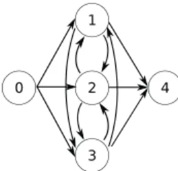
Two dummy jobs j=0 andj=n+1 are used as ﬁrst and last job of the sequences. These dummy jobs do not have any pro-cessing time and no setup is required. Figure 1 is visualizing this formulation on the example of three jobs using a graph rep-resentation. Each node represents a job, including the dummy start job (0) and the dummy end job (n+1=4). The arcs repre-sent the decision variablesxi,j. In case e.g. job 2 is sequenced

before job 3 in a solution, the binaryx2,3is set to 1 and the arc

between job 2 and job 3 is used.

Fig. 1. Graph representation of the 2-index formulation with n=3 jobs (1,2,3) and the dummy start job (0) as well as the dummy end job (n+1). The decision variablesxi,jare represented by the arcs.

The problem is minimize n j=1 Tj (1) subject to n i=0 xi,j=1 forallj=1, ..,n+1 (2) n+1 j=1 xi,j=1 foralli=0, ...,n (3) xj,j=0 for allj=1, ...,n (4) C0=0 (5) Cj≥Ci+si,j+pj−(1−xi,j)M foralli=0, ...,n,j=1, ...,n+1 (6) Cj≤Ci+si,j+pj+(1−xi,j)M foralli=0, ...,n,j=1, ...,n+1 (7) Tj≥Cj−djforall j=1, ...,n (8) Tj≥0 forallj=1, ...,n (9) xi,j∈ {0,1}foralli=0, ...,n,j=1, ...,n+1 (10)

The objective (1) is to minimize the sum of tardiness of all jobs in the production schedule. Constraints (2) describes that each jobjhas exactly one predecessor. Constraint (3) ensures that each jobihas exactly one successor and (4) makes sure that each job is only used once. Together the ﬁrst three con-straints describe a valid permutation of all jobs. Constraint (5) initializes the completion time of the dummy start job. Con-straints (6) and (7) calculate the completion times of all jobs in the sequence. The big-M formulation is used to turn the con-straint on or oﬀ, depending on whether job j is immediately following jobiwithxi,j=1 or not. Constraints (8) and (9) are

calculating the tardiness of each job. Constraint (10) constrains the domain of the decision variables.

The large number M used to turn constraints (6) and (7) on or oﬀcan theoretically be set arbitrarily large, however, too large values can cause numerical problems in the solution

(3)

pro-cess [14]. By setting M=nmaxn i,j=1si,j+ n j=1 pj (11)

we can ensure that M is greater then any completion time pos-sible, thus, being large enough to be usable for constraints (6) and (7).

2.2. 3-index Formulation

Again, a set ofnjobs is given. Each job is characterized by a due datedj, a processing timepj, and a setup family fj.

The 3-index formulation is a position-based model using binary decision variablesxk

i,j, which equal 1 if jobjis scheduled at the

kth position in the sequence and immediately follows jobiand

equal 0 otherwise. With the explicit description of the position in the sequence, we can denote withCkthe completion time

of the job in positionkand withTkthe resulting tardiness of

the job in positionk(this formulation is based on [12] and also used for the exact method developed in [4]). Again, we use for each pair of jobsiand j, the parametersi,jindicating the setup

time required if job jfollows jobi, i.e. si,j = sf if fi fj

andsi,j = 0 otherwise. The 3-index formulation also uses a

dummy start jobj=0 and a dummy ﬁnishing jobj=n+1 for modeling purposes. The 3-index formulation is displayed as a graph representation in Figure 2. Each node (i,k) represents a certain jobiin a speciﬁc sequence positionk. The arcs represent the binary decision variablesxk

i,j.

The problem is

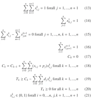
Fig. 2. Visualization of the 3-index formulation with n=3 jobs (1,2,3) and the dummy start job (0 at position k=0) as well as the dummy end job (n+1, at position k=4). Each job can be sequenced at one of the available positions k=1,2,3. minimize n k=1 Tk (12) subject to n i=0 n+1 k=1 xki,j=1 forallj=1, ...,n+1 (13) n j=1 x1 0,j=1 (14) n i=0 xk i,j− n+1 m=1 xk+1 j,m =0 forallj=1, ...,n,k=1, ...,n (15) n i=1 xn+1 i,n+1=1 (16) C0=0 (17) Ck=Ck−1+ n i=0 n j=1 (si,j+pj)xik,jforallk=1, ...,n (18) Tk≥Ck− n i=0 n j=1 djxki,jforallk=1, ...,n (19) Tk≥0 for allk=1, ...,n (20) xk i,j∈ {0,1}foralli=0, ...n,j,k=1, ...,n+1 (21)

The objective (12) is again to minimize the sum of tardiness of all jobs in the production schedule. Constraint (13) makes sure that each job j is fulfilled exactly once, by only allow-ing one predecessoriin exactly one positionkof the sequence. Constraint (14) defines exactly one jobjto be the first job after the dummy start jobj=0. Constraint (15) ensures flow of jobs from starting jobj=0 to the finishing jobj=n+1, without allowing sub circles to appear. Analogous to constraint (14), constraint (16) defines exactly one jobito be the last job se-quenced before the finishing jobj=n+1. Constraints (17) ini-tializes the completion time of positionk=0, i.e. the position of dummy jobj=0. Constraint (18) calculates the completion time for each positionkof the sequence. Constraints (19) and (20) calculate the resulting tardiness for each positionk. The decision variables are bounded by constraint (21).

2.3. Comparison of the Formulations

The 2-index and 3-index formulation presented above strongly diﬀer in the number of variables. In the 2-index for-mulation there aren2₊_2n₊_{1 binary variables. Furthermore,}

there are 2n+1 linear variables and 2n2₊_9n₊_{7 constraints. On}

the other side, the 3-index formulation hasn3₊_3n2₊_3n₊₁

bi-nary variable, 2n+1 linear variables, andn2₊_4n₊_{4 constraints.}

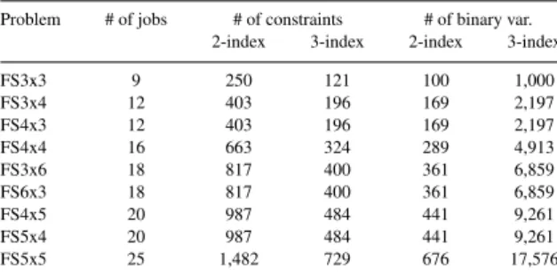
An overview of the number of constraints and binary variables for the different test sets is displayed in the next section in Table 1. Due to the significantly smaller number of binary variables one may assume that it is favorable to use the 2-index formu-lation. However, the solution space of the 2-index formulation differs in the structure due to the conditional constraints (6) and (7) which are linearized using the so-called big-M notation. As we will see in the remainder, this difference in the structure of the solution space makes it difficult to find good lower bounds quickly and is thus an obstacle in solving the problem. By using the additional index, indicating the job’s position in the

(4)

Table 1. Number of constraints and binary variables for each problem Problem # of jobs # of constraints # of binary var.

2-index 3-index 2-index 3-index

FS3x3 9 250 121 100 1,000 FS3x4 12 403 196 169 2,197 FS4x3 12 403 196 169 2,197 FS4x4 16 663 324 289 4,913 FS3x6 18 817 400 361 6,859 FS6x3 18 817 400 361 6,859 FS4x5 20 987 484 441 9,261 FS5x4 20 987 484 441 9,261 FS5x5 25 1,482 729 676 17,576

sequence, the 3-index formulation does not require the big-M notation to calculate the completion times.

3. Experiment Design

Although, there are test sets available for scheduling problems with setup times between diﬀerent jobs([15] and [8]), we are not aware of any available test instances for the family scheduling problem. However, [16][10] and [6] provide descriptions of the test instances they used in their papers. For our experiments we replicated test sets using the methodology and parameters proposed by Schaller[16]. These replicated test instances used in this paper can be accessed at www. jacobs-university.de/ses/distributionlogistics/ research/continuouscasting.

Each test set is described by the number of families nf and the number of jobs in each familynj f. For this paper an equal distribution of jobs to families is assumed. The diﬀerent problems are named FS for family scheduling followed by

nfXnj f. [16] generates his test instances by varying the range of setup times, a due date rangeRand a tardiness factorr. Both

Randrare used when calculating the job due dates. Since the focus of this paper is to compare the two formulations, rather then testing one formulation for diﬀerent settings, the problems are generated usingR=1,r=0.5 in the formulation given by

the author. The range for the setups is [1,20], and processing times are derived from the range [1,10]. Nine diﬀerent instance sets have been created with bothnf andnj fvarying between 3 and 6. The resulting number of jobs is between 9 and 25. Table 1 provides an overview of the selected problems. For each set, ﬁve test instances were generated. When applying both formulations to the test instances, a total of 90 experiments were carried out.

Table 1 shows the diﬀerences in problem size between the 2-index and the 3-index formulation. While the number of con-straints only diﬀers by a factor of two, the 3-index formulation needs a much larger amount of binary variables to describe the problem. For the largest experiment with 25 jobs, this results in 17,575 binaries for the 3-index formulation in comparison to 676 binary variables in the 2-index case.

All problem instances are solved using the commercial MIP solver CPLEX in version 12.6. This solver is using a B&B procedure to solve the minimization MIP problem. Lower bounds are calculated by solving the linear programming (LP) relaxation of the problems original IP problem. These

bounds are used to fathom unpromising branches in the search tree. Branches are generated when the LP relaxation leads to fractional decision variables, e.g. x7,13 =0.5361 leads to one sub problem with x7,13 = 0 and another withx7,13 = 1. In order to avoid excessive growth of branches in the search tree, the problem formulation must enable the solver to calculate ”good” lower bounds. This is the case when the LP relaxation is close to the integer problem ([19]). Constraints that narrow the search space but not exclude valid integer solutions , reduce the gap between LP and IP. In case it is possible to describe the so called convex hull of the integer problem, i.e. introducing all inequalities that describe the valid integer points at the outline of the search space, then the LP is equal to the IP problem and the solution to the IP can be obtained by solving the easier LP problem [13]).

The experiments where carried out on an Intel Xeon(R) CPU W3530 @ 2.80GHz 4 with UBUNTU 12.04 32-bit operating system, using 3 threads and 2GB system RAM. In order to be able to process larger test instances, the solvers function to cre-ate nodes using hard disc space was applied to a total limit of 10GB per experiment. As in Baker and Keller[3] we used a one hour time limit for each test instance, measured in CPU time. In case the optimal solution has not been found within the time limit, the run was terminated and the current upper and lower bound were collected to calculate the gap as a measure of close-ness to the optimal solution. All other parameters available to adjust the CPLEX solver were left in the default conﬁguration.

4. Numerical Results and Discussion

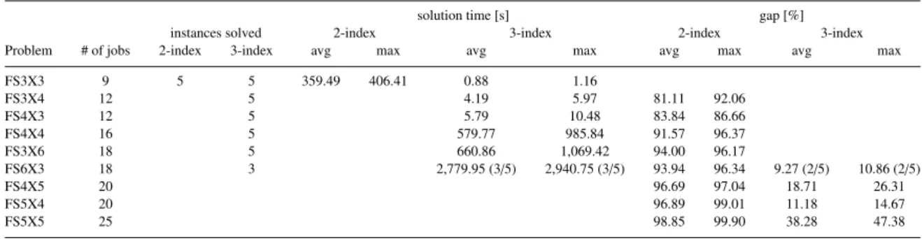
The results for the nine instance sets are shown in Table 2. For each problem, the name, the number of jobs, the number of solved instances, the solution time in seconds and the gap between upper bound and lower bound are shown for both for-mulations (2-index and 3-index). Since each set consists of ﬁve randomly generated test instances, average and maximum val-ues for all test instances are reported per test set. If some of the instances were not solved within the time limit, we indicate the solution time for those instances which are solved and indicate in brackets how many of the ﬁve instances are solved. For in-stances which are solved not within the time limit of one hour, we report the gap analogously. Blanks are displayed for the so-lution time in case no instance was solved, and for the gap in case all instance of a problem have been solved.

The results show that the 3-index formulation is superior for all instance sets. The 3-index formulation was able to solve all test instances with up to 16 jobs within the calculation time limit of one hour. The 2-index formulation only solved the smallest test instances with 9 jobs. Only some of the instances with 18 jobs are solved for the 3-index formulation and larger instances are not solved for either formulation. Still, the 3-index formulation provided much closer gaps and therefore closer ap-proximations of the optimal solution.

The results for alternative test instances within the same set show some variation. For instance setFS6X3, three instances were solved for the 3-index formulation, one within less than 2,600 seconds, while another could not been solved and ter-minated with a gap of 10.86%. For instance setFS3X6, the fastest instance was solved in less than a minute (56 seconds),

(5)

Table 2. Calculation times and gap between upper and lower bound for each problem

solution time [s] gap [%]

instances solved 2-index 3-index 2-index 3-index

Problem # of jobs 2-index 3-index avg max avg max avg max avg max

FS3X3 9 5 5 359.49 406.41 0.88 1.16 FS3X4 12 5 4.19 5.97 81.11 92.06 FS4X3 12 5 5.79 10.48 83.84 86.66 FS4X4 16 5 579.77 985.84 91.57 96.37 FS3X6 18 5 660.86 1,069.42 94.00 96.17 FS6X3 18 3 2,779.95 (3/5) 2,940.75 (3/5) 93.94 96.34 9.27 (2/5) 10.86 (2/5) FS4X5 20 96.69 97.04 18.71 26.31 FS5X4 20 96.89 99.01 11.18 14.67 FS5X5 25 98.85 99.90 38.28 47.38

while the slowest took more than 15 minutes (1,069 seconds). There is also a diﬀerence in the results of instances setsFS6X3 andFS3X6, although both have 18 jobs in total. For instances in setFS6X3 the jobs are distributed over six families, while there are only three families for instances in setFS3X6. Less families, in this case, were much better solvable. ForFS3X6, all instances are solved with an average calculation time of 661 seconds, while forFS6X3 only three instances are solved in 2,780 seconds on average.

When examining the results in more details, it can be ob-served that the 2-index formulation is able to derive strong up-per bounds, often even the optimal solutions. The reason for the poor performance of the 2-index formulation shown in Table 2 origins from the inability to derive sufficient lower bounds to proof optimality. Table 3 shows the average upper and lower bounds over all five test instances for each problem. While the upper bounds only differ by 0.14% over all problems, the lower bounds differ by 88.53%. The utilization of the big-M notation in the 2-index formulation appears to have a strong negative impact on generating good lower bounds. [7] state that big-M coefficients only marginally influence the LP relaxation results. That means the constraints are not able to contribute to a realis-tic bound calculation. At the same time, the additional variables and constraints even hinder the B&B solution process. Table 3. Average Upper and Lower Bounds over all five Instances per Problem

upper bound lower bounds Problem # of jobs 2-index 3-index 2-index 3-index

FS3X3 9 248.60 248.60 248.60 248.60 FS3X4 12 320.60 320.60 63.16 320.60 FS4X3 12 319.60 319.60 52.28 319.60 FS4X4 16 586.00 586.00 52.67 586.00 FS3X6 18 676.60 676.00 41.89 676.00 FS6X3 18 732.40 739.60 43.86 714.44 FS4X5 20 679.20 677.40 22.51 549.11 FS5X4 20 852.80 852.60 29.46 757.93 FS5X5 25 1201.00 1204.00 14.66 749.77

Another interesting observation can be made when analyz-ing the root calculation performance of the diﬀerent problems for both formulations. Table 4 shows the calculation time for the initial LP relaxation as well as the entire time needed to process the root node. This includes solvers internal model generation and preprocessing operations. The time needed to calculate the initial LP relaxation is a good indicator for the

ef-fort of calculating lower bounds for all roots within the B&B procedure.

Table 4. Total Root Processing and LP Relaxation Calculation Times average root calculation time [s] LP relaxation total root processing Problem # of jobs 2-index 3-index 2-index 3-index

FS3X3 9 <0.01 0.01 0.19 0.84 FS3X4 12 <0.01 0.04 0.25 2.55 FS4X3 12 <0.01 0.04 0.24 2.16 FS4X4 16 <0.01 0.63 0.42 10.29 FS3X6 18 <0.01 1.33 0.57 15.01 FS6X3 18 <0.01 1.18 0.59 15.92 FS4X5 20 <0.01 2.19 0.76 20.88 FS5X4 20 <0.01 1.40 0.69 19.53 FS5X5 25 <0.01 4.47 1.65 39.62

The ﬁrst observation is that with the 2-index formulation the LP relaxation can be calculated in very short time, even for the largest problem instances examined. For the 3-index formula-tion much more time is required to process the root node. While the diﬀerence is rather small for problems with few jobs, it in-creases rapidly when the problem size inin-creases. When dou-bling the problem size from 12 to 25, the time needed to cal-culate the LP relaxation increases from 0.04 seconds to 4.47 seconds. The same holds for the initial total root processing. With 39.62 seconds, instance setFS5X5 already used 1.1% of the given calculation time limit.

5. Conclusions

This paper compares two alternative integer programming formulations of the single machine family scheduling problem. One formulation is a typical sequence based 2-index formula-tion while the other is a posiformula-tion based 3-index formulaformula-tion. Computational experiments are conducted on 45 test instances with diﬀerent characteristics.

Although the 2-index formulation uses a signiﬁcantly smaller amount of binary variables, it is clearly outperformed by the index formulation for the given test sets. For the 3-index formulation we were able to solve 28 out of 30 instances with up to 18 jobs to optimality, for the 2-index formulation only the smallest instances with 9 jobs were solved within the time limit of one hour. For those instances which were not solved in the time limit, the 3-index formulation has a much

(6)

better optimality gap.

Even though the development of sophisticated and tailor made solution approaches for industrial problems is often not possible, our research shows that by using better models larger problems can be solved faster. Practitioners without specific al-gorithmic knowledge can easily test and evaluate different mod-eling approaches using commercial multi-purpose MIP solvers. This paper shows that the benefit can be significant.

References

[1] A. Allahverdi and H. Soroush. The signiﬁcance of reducing setup times/setup costs.European Journal of Operational Research, 187(3):978– 984, June 2008.

[2] A. Allahverdi, C. Ng, T. Cheng, and M. Y. Kovalyov. A survey of schedul-ing problems with setup times or costs.European Journal of Operational Research, 187(3):985–1032, June 2008.

[3] K. R. Baker and B. Keller. Solving the Single-Machine Sequencing Prob-lem using Interger Programming.Computers&Industrial Engineering, 59 (4):730–735, 2010.

[4] L.-P. Bigras, M. Gamache, and G. Savard. The time-dependent traveling salesman problem and single machine scheduling problems with sequence dependent setup times.Discrete Optimization, 5(4):685–699, Nov. 2008. [5] S. Y. Chang, M.-R. Chang, and Y. Hong. A lot grouping algorithm for a

continuous slab caster in an integrated steel mill.Production Planning& Control, 11(4):363–368, Jan. 2000.

[6] S. Chantaravarapan.Heuristics for the family scheduling problems to min-imize total tardiness. PhD thesis, Texas Tech University, 2002. [7] G. Codato and M. Fischetti. Combinatorial Benders Cuts for Mixed-Integer

Linear Programming.Operations Research, 54(4):1–22, 2006. [8] C. Gagn´e, W. Price, and M. Gravel. Comparing an ACO algorithm with

other heuristics for the single machine scheduling problem with sequence-dependent setup times. Journal of the Operational Research Society, 53 (8):895–906, 2002.

[9] R. L. Graham, E. L. Lawler, J. K. Lenstra, and A. H. G. R. Kan. Opti-mization and approximation in deterministic sequencing and scheduling: a survey.Annals of Discrete Mathematics, 5287–326, 1977.

[10] J. N. D. Gupta and S. Chantaravarapan. Single machine group scheduling with family setups to minimize total tardiness. International Journal of Production Research, 46(6):1707–1722, Mar. 2008.

[11] M. M. Liaee and H. Emmons. Scheduling families of jobs with setup times. International Journal of Production Economics, 51:165–176, 1997. [12] J. Picard and M. Queyranne. The time-dependent traveling salesman

prob-lem and its application to the tardiness probprob-lem in one-machine scheduling. Operations Research, 26(1):86–110, 1978.

[] M. Queyranne and A. S. Schulz. Polyhedral Approaches to Machine Scheduling. 1994.

[14] P. A. Rubin. Heuristic solution procedures for a mixedinteger programming discriminant model.Managerial and Decision Economics, 11(4):255–266, 1990.

[15] P. A. Rubin and G. L. Ragatz. Scheduling in a sequence dependent setup environment with genetic search. Computers&Operations Research, 22 (1):85–99, 1995. que

[16] J. E. Schaller. Scheduling on a single machine with family setups to mini-mize total tardiness. International Journal of Production Economics, 105 (2):329–344, Feb. 2007.

[17] S. Tanaka and M. Araki. An exact algorithm for the single-machine total weighted tardiness problem with sequence-dependent setup times. Com-puters&Operations Research, 40(1):344–352, 2013.

[18] K. Windt, P. Nyhuis, and O. Herr. Exploring eﬀects of sequencing modes towards logistics target achievement on the example of steel production. Procedia CIRP, 3:620–625, 2012.