Global Constraints in Distributed Constraint
Satisfaction and Optimization
Christian Bessiere
1Ismel Brito
2Patricia Gutierrez
2Pedro Meseguer
2 1University of Montpellier
[email protected]
2
IIIA - CSIC, Universitat Aut`onoma de Barcelona
[email protected], [email protected], [email protected]
Abstract
Global constraints are an essential component in the efficiency of centralized constraint programming. We propose to include global constraints in distributed constraint satisfaction and optimization problems (DisCSPs and DCOPs). We de-tail how this inclusion can be done, considering different representations for global constraints (direct, nested, binary). We explore the relation of global constraints with local consistency (both in the hard and soft cases), in particular for general-ized arc consistency (GAC). We provide experimental evidence of the benefits of global constraints on several benchmarks, both for distributed constraint satisfac-tion and for distributed constraint optimizasatisfac-tion.
1
Introduction
With the rise of Internet, there are more and more opportunities to solve problems in a distributed form. Distribution implies that different problem parts are handled by different agents, and these parts cannot be joined in a single agent for a centralized solving. This new setting requires the adaptation of existing solving strategies or the generation of new ones. Often, problems are solved by message passing [1].
The same trend is observed in constraint programming. A strong motivation for distributed constraint solving is privacy. Constraints contain information that agents may desire to keep hidden from other agents, which could be seen as competitors. Usually, it is assumed that a constraint is known by the agents involved in it, but not by the other agents [2]. Distributed constraint reasoning appears as a natural extension of the usual centralized approach to constraint reasoning, keeping its solving capabilities but removing the implicit assumption that every detail of the instance is known by the solving agent. In the last years a number of distributed algorithms have been proposed: ABT [2], AFC [3] ADOPT [4], NCBB [5], among others.
In centralized constraint reasoning, global constraints have been an essential com-ponent of the efficiency of constraint solvers [6]. A global constraintC is a class
of constraints that all have the same specific semantics but that can involve any (un-bounded) number of variables. The standard example is theall-differentconstraint, that requires that all the involved variables must take a different value. You can apply this constraint to sets of variables of any size. Each application is considered as a constraint instance. The exploitation of the semantics associated with a global constraint allows to design specialized propagators able to reach local consistency levels (typically general-ized arc consistency), usually with lower complexity than generic propagators. Current constraint solvers include a list of global constraints, with propagators already imple-mented, available for the user to model and solve her problem [7].
Often, it is implicitly assumed that distributed constraint reasoning precludes the use of global constraints. The usual assumption is that an agent knows the constraint with each of its neighbors separately, and nothing else [2, 4]. These constraints are obviously binary. However, this interpretation is too restrictive because there are dis-tributed applications for which it is natural to use global constraints. For example, let us consider a distributed meeting scheduling problem where agenta1is trying to
find an appointment with agentsa2anda3. Agenta1may easily infer that there is an all-equalconstraint betweena1,a2anda3.
When adding global constraints in distributed reasoning we obtain several benefits. First, the expressivity of distributed constraint reasoning is enhanced because there are relations among variables with a particular meaning that cannot be expressed as a con-junction of binary relations (there are global constraints that are not binary decompos-able). Second, the solving process can be done more efficiently. Local consistency can be enforced more efficiently when global constraints are involved [6]. Hence, assuming a solving strategy maintaining some kind of local consistency, the inclusion of global constraints improves the efficiency of the solving process, requiring less computational resources.
Once the interest of global constraints in distributed constraint reasoning is ac-cepted, another question naturally follows: since some global constraints can be de-composed in simpler constraints, what is more efficient, to leave the global constraint as it was initially posted or to decompose it? If several decompositions are possible, which offers the best performance? We provide some answers to these questions, ex-ploring two kinds of decompositions (binary [8] and nested for contractible constraints [9]) against the global constraint without decomposition, in two contexts: complete distributed search with / without unconditional GAC maintenance [10].
Previous paragraphs have introduced what we consider as the two main contri-butions of this paper: (i) the inclusion of global constraints in distributed constraint reasoning, and (ii) the exploration of different representations for global constraints in a distributed context, looking for the most efficient one. To perform this task, we use state-of-the-art distributed constraint solving algorithms, which have already been combined with some form of local consistency [10, 11, 12].
All what we have said equally applies tohardglobal constraints (global constraints which should mandatorily be satisfied, satisfaction case) and tosoftglobal constraints, (global constraints which should be satisfiedas much as possible, optimization case). Although the satisfaction case can be seen as a special case of the more general opti-mization one, the former uses different algorithmic techniques. For this reason, in the following, after giving motivation (Section 2) and background for this work (Section
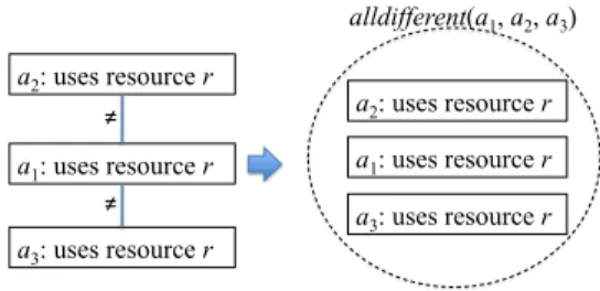
a2: uses resource r a1: uses resource r a3: uses resource r alldifferent(a1, a2, a3) ! ! a2: uses resource r a1: uses resource r a3: uses resource r
Figure 1: Job-shop scheduling problem, where agentsa1, a2, a3 share the same
re-sourcer. To determine its starting time, agenta1 knows it must be different froma2
anda3. But because they use the same resourcer,a1can deduce that there is a global all-differentconstraint among them.
3), we treat separately the inclusion of hard global constraints in distributed constraint satisfaction (Section 4) and the inclusion of soft global constraints in distributed opti-mization (Section 5). In Section 6 we terminate with some conclusions of this work.
2
Motivation
2.1
Satisfaction Case
In distributed constraint satisfaction (DisCSP) agents cooperate to find a global solu-tion. It is assumed that each agent knows a part of the problem (the variables owned by the agent and the constraints in which they are involved) but no agent knows the whole problem. Often it is also implicitly assumed that constraints are binary, under the idea that an agent relates with another agent independently of how it relates with others. However, this view precludes the use of global constraints. In some situations global constraints naturally appear in the distributed context.
First, a global constraint appears in DisCSP when an agent can infer the existence of a global constraint from the task it performs and from the existence of some other constraints (usually binary). For example, consider the distributed job-shop scheduling problem. If agenta1is trying to set up the starting time of its task which uses resource r, with other two agentsa2anda3which also use the same resource,a1may deduce
that there is anall-differentconstraint betweena1,a2anda3. This example appears in
Figure 1.
Second, a global constraint appears in DisCSP when the model designer informs the agents of the existence of that global constraint. This information is needed to properly accomplish the intended task. For example, let us consider the task of a PC configura-tion, which consists in selecting a motherboard and a number of options according to the user desires. A motherboard for PC contains the CPU plus slots for memory cards, slots for disks (hard disks and DVDs), and slots for any other device. Configuring a PC means deciding which motherboard to choose and which devices are connected to the motherboard slots, satisfying the user specification. A natural constraint model of this problem contains variables for the motherboard and its slots. A solution means
selecting the values for these variables, such that all constraints are satisfied. There are a number of technical constraints: only 1 motherboard, binary constraints between the motherboard and the other PC elements (memories, disks, etc.) ensuring compati-bility, at least one hard disk is needed (to perform system bootstrapping). In addition, there are a number of global constraints among variables representing elements of the same type (or connecting to the same slot type) establishing the desired minimum and maximum number of elements according to the user specification (atleastandatmost
constraints). Other global constraints may exist on the total desired capacity of a par-ticular element and on the maximum budget (sumconstraint).
Following with this example, let us consider a multi-agent context. There are several agents providers of motherboards(C1, ..., Cp), memories(M1, ..., Mq), disks
(D1, ..., Dr), and other devices(O1, ..., Os). We group agents in four sorts,c, m, d, o,
for providers of motherboards, memories, disks and other devices. Each agent has four vectors of variablesid[1...Ks],type[1... Ks],capacity[1...Ks],price[1...Ks]. Ks al-lows enough elements for the maximum number of slots of sortsin any motherboard; for motherboard providers these vectors have 1 element only. The obvious meaning of these vectors is: id[i]is an item of typetype[i]with capacitycapacity[i]and price
price[i]. This is ensured by a quaternary constraint on id[i],type[i],capacity[i] and
price[i], for alliin1..Ks. There is a special valueemptyforid[i]andtype[i], which forcescapacity[i]andprice[i]to be zero. Typically,idcontains the item identifier, ac-cording to the provider catalog, whiletypeindicates the type of device or connection, with the following values:motherboard, memory card, hard disk, DVD, microphone, speakers, printer, ethernet, USB. Incapacityit is stored the processor speed, the mem-ory card size or the hard disk capacity. Fortype = DVD,capacityis 0.
We use the following global constraints in the modelling: atleast [t, v](Vars) (valuev has to appear at least t times in the assignment of the variables inVars),
atmost[t, v](Vars)(valuevhas to appear at mostttimes in the assignment ofVars),
exactly[t, v](Vars) =atleast[t, v](Vars)∧atmost[t, v](Vars),sum(Vars)≤bound
(the sum ofVarsis lower than or equal tobound),sum(Vars)≥bound(the sum of
Varsis greater than or equal tobound).
Let us consider the following PC specification: CPU speed≥2.5 GHz; memory between 8GB and 16GB; at most 2 hard disks; total disk storage≥1TB; 1 DVD; at least 1 ethernet connection; at least 1 printer connection; at least 2 USB; maximum budget$500. This specification is translated into the following constraints:
1. Unary constraint oncapacity[1] variable of motherboard providers:
capacity[1]≥2.5GHz.
2. Only one motherboard is required:
exactly[1,motherboard](typevars ofC1, ..., Cp).
3. Binary compatibility constraints: between motherboard providers and providers of any other element.
4. Assuming that memory cards for any provider are standard with the same size (4GB), memory specifications can be translated into number of cards among all mem-ory providers:
atleast[2, memory card](typevars ofM1, ..., Mq) atmost[4, memory card](typevars ofM1, ..., Mq)
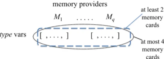
M1 Mq [ , . . . , ] [ , . . . , ] . . . type vars memory providers at least 2 memory cards at most 4 memory cards
Figure 2: Memory configuration in a multi-agent context, as explained in the text.
M1, ..., Mq are memory provider agents. Each has a vector oftype variables, con-taining the memory cards to be used in the configuration. Following user spec-ification, there are two global constraints, atleast[2, memory card](type vars of
M1, ..., Mq), atmost[4, memory card](typevars ofM1, ..., Mq). Since these con-straints are not binary decomposable, there is no set of binary concon-straints on the prob-lem variables with the same meaning.
5. Constraints on the number of hard disks:
atleast[1, hard disk](typevars ofD1, ..., Dr)
atmost[2, hard disk](typevars ofD1, ..., Dr)
6. Exactly one DVD:exactly[1, DV D](typevars ofD1, ..., Dr)
7. Total hard disk storage:
sum(capacityvars ofD1, ..., Dr)≥1TB
8. At least one ethernet connection:
atleast[1, ethernet](typevars ofO1, ..., Os)
9. At least one printer connection:
atleast[1, printer](typevars ofO1, ..., Os)
10. At least two USB ports:atleast[2, U SB](typevars ofO1, ..., Os)
11. Budget limited to $500:
sum(pricevars of all providers)≤$500
Constraints 2 and 4–11 are global constraints on the number, capacity or price of the PC components.
A final example comes from the sensor network application reported in [13]. There are a set of sensors and a set of mobiles. The goal is to track each mobile with 3 sensors, under some constraints of visibility (between sensors and mobiles) and compatibility (among sensors). In the model of [13], agents are mobiles, containing three variables for the three tracking sensors. If global constraints are allowed it becomes possible to provide a more natural model of this problem with sensors as agents, under anatleast
global constraint requiring at least 3 sensors to track each mobile.
In summary, an agent may be related by one or several global constraints together with a subset of the agents. This information can be deduced by the agent, or pro-vided by an external source. Although binary constraints are the obvious choice in dis-tributed constraint reasoning, some global constraints can also be used for modelling and solving these problems. In some cases, global constraints are needed for expressiv-ity requirements. By exploiting global constrains some efficiency improvements can
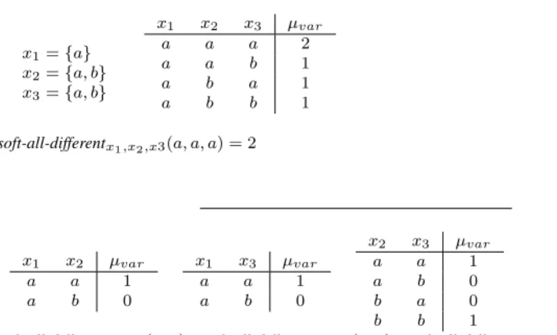
x1={a} x2={a, b} x3={a, b} x1 x2 x3 µvar a a a 2 a a b 1 a b a 1 a b b 1 soft-all-differentx1,x2,x3(a, a, a) = 2 x1 x2 µvar a a 1 a b 0 x1 x3 µvar a a 1 a b 0 x2 x3 µvar a a 1 a b 0 b a 0 b b 1
soft-all-differentx1,x2(a, a)+soft-all-differentx1,x3(a, a)+soft-all-differentx2,x3(a, a) = 3
Figure 3: (Top)soft-all-differentsoft global constraint withµvar violation measure; (bottom) its binary decomposition
be achieved.
2.2
Optimization Case
A soft global constraint is a global constraint plus a violation measure that defines the costs of value assignments based on the semantics of the global constraint and the amount of violation. For example, thesoft-all-different(T)is associated with the violation measureµvar, defined as the number of variables inT that have to change their value to satisfy that all values are different. Another violation measure for soft-all-differentisµdec, defined as the number of pairs of variables inT with the same value [14].
As in the satisfaction case, binary soft constraints is a common assumption. How-ever, not every soft constraint can be decomposed into an equivalent set of binary ones. For example, consider thesoft-all-differentsoft global constraint in Figure 3 defined over variablesx1, x2, x3. The cost of every value tuple is defined by the violation
mea-sureµvar. Observe that the tuple{x1=a, x2=a, x3=a}has a different cost in the
global formulation —involving all variables— and in the binary formulation. Hence, this constraint is not binary decomposable with the violation measureµvar.1 In gen-eral, most soft global constraints are not binary decomposable, so working with their global formulations is crucial for their effective inclusion in DCOPs.
3
Background
In this section we introduce all the necessary material on distributed reasoning and global constraints, both in the case of satisfaction problems and in the case of
opti-1Notice, however, that thesoft-all-differentconstraint is binary decomposable with the violation measure
mization problems.
3.1
Satisfaction
CSP.AConstraint Satisfaction Problem(CSP) consists in finding solutions to a con-straint network. Aconstraint networkis a tuple(X,D,C)whereX ={x1, . . . , xn} is a set ofnvariables,D={D(x1), . . . , D(xn)}is a set of finite domains such that
D(xi)is the value set forxi, andCis a finite set of constraints. A constraintC(T)∈ C on the ordered subset of variablesT = (xi1, . . . , xir(i))specifies the set of tuples on
xi1, . . . , xir(i) allowed by C(T). The set of allowed tuples can be defined by a table
in extension, or by any Boolean function. Asolutionis an assignment of values to variables which satisfies every constraint. Solving a CSP is NP-complete.
Generalized Arc Consistency. Given a constraintC(T), a pair(xi, a),xi ∈T,a∈
D(xi)isgeneralized arc consistent(GAC) with respect toC(T)if there exists a tuple
tonTsuch that the projectiont[xi]oftonxiisa,tis allowed byC(T), and for every
xj ∈T, j6=i,t[xj]∈D(xj);tis asupportofawith respect toC(T). Variablexiis GAC if all its values are GAC with respect to every constraint involvingxi; a CSP is GAC if every variable is GAC.
Global Constraints.Aglobal constraintcaptures a relation with a specific semantics that can apply on any number of variables [6]. C is a class of constraints defined by a Boolean functionfC whose arity is not fixed. Constraints with different arities can be defined by the same Boolean function. For instance,all-different(x1, x2, x3)
andall-different(x1, x4, x5, x6)are two instances of theall-differentglobal constraint,
wherefall-different(T)returns true iffxi 6=xj,∀xi, xj ∈ T. In [9], Maher has defined the property ofcontractibility. A global constraintCiscontractibleiff for any tuplet
onxi1, . . . , xip+1, iftsatisfiesC(xi1, . . . , xip+1)then the projectiont[xi1, . . . , xip]of tonxi1, . . . , xipsatisfiesC(xi1, . . . , xip)[9].
In [8], Bessiere and Van Hentenryck defined the property ofdecomposability with-out extra variables. A global constraintCisbinary-decomposable without extra vari-ablesiff for any instanceC(T)ofC, there exists a setSof binary constraints involving only variables inTsuch that the solutions ofSare the solutions ofC(T)[8].Sis called abinary decompositionofC(T).
DisCSP.ADistributed Constraint Satisfaction Problem(DisCSP) is a 5-tuple(X,D,
C,A,φ), whereX,DandCform a CSP whose variables, domains and constraints are distributed among automated agents. In addition,A={1, . . . , p}is a set ofpagents, andφ:X → Ais a function that maps each variable to its agent. We make the usual assumption that each agents owns exactly one variable, so agents and variables can be used interchangeably. We also assume that a constraintC(T)among several variables is known by every agent that owns a variable ofT [2]. The set of constraints known by agentiis writtenCi. As in the centralized case, asolutionis an assignment of values to variables satisfying every constraint. DisCSPs are solved by the coordinated action of agents, which communicate through messages. It is assumed that the delay of a message is finite but random. For each pair of agents, message delivery follows the sending order.
ABT.Asynchronous Backtracking(ABT) [2] is the reference algorithm for DisCSPs, with a role similar to backtracking in centralized CSPs. ABT is purely asynchronous,
each agent makes its own decisions, informs other agents about them, and no agent has to wait for the others’ decisions. An ABT agent computes a global consistent solution (or detects that no solution exists) in finite time; its correctness and completeness have been proved [2, 15].
ABT requires a total order among agents, inducing a direction in the constraints. A binary constraint causes a directed link between the two constrained agents: the value-sending agent, from which the link starts, to the constraint-evaluating agent, at which the link ends. Each ABT agent keeps its own agent view and nogood store. The agent view of a generic agentself is the set of values thatself believes are assigned to higher priority agents (connected toself by incoming links). Its nogood store keeps nogoods as justifications of inconsistent values. Anogoodis a conjunction of assignmentsxi =
a∧xj =b∧. . . xk =c∧xp =dthat is inconsistent, that is, it violates at least one constraint. Often a nogood is written in directed form, asxi =a∧xj =b∧. . . xk =
c ⇒ xp 6= d, wherexpshould be considered after all other nogood variables in the search tree. The left-hand side (lhs) of the nogood is the expression that appears at the left side of the implication, while the right-hand side (rhs) appears at the right of the implication. Agents exchange four types of messages:
• OK?(i, j, val):iinformsjthat it has taken valueval;
• NGD(j, i, ng): jinformsithat it has detected nogoodngthat involvesias the last agent in the order;
• ADDL(i, j):iasksjto set up a link fromjtoi;
• STOP(i, j): iinformsjthat the empty nogood has been generated and there is no solution.
Agents inform of their assignments by sending OK? messages to lower priority agents, which try to accommodate their assignments to the values taken by higher priority agents. If this is not possible, the lower priority agent sends a NGD message to the lowest higher priority agent in the new nogood generated [2]. If an unconnected agent appears in the nogood, it is requested to set up a new link using the ADDL message.
When ABT starts, each agent assigns its variable, and sends OK? messages con-taining its assignment to its neighboring agents with lower priority. Whenself receives an OK? message,self updates its agent view with the new assignment, removes no-goods which are inconsistent with this new assignment and checks the consistency of its own current assignment with the updated agent view.
Whenself receives a NGD message, it is accepted if the contained nogood is con-sistent withself’s agent view (values of the common variables in the nogood and in
self’s agent view are the same). Otherwise,self discards the nogood as obsolete. If the nogood is accepted, the nogood store is updated, causingself to search for a new con-sistent value (since the received nogood forbids its current value). If an unconnected agentiappears in the nogood, it is requested to set up a new link withself, by the mes-sage ADDL (sent fromself toi). From this point on,self will receive the values taken byi. Whenself cannot find any value consistent with its agent view, either because of the original constraints or because of the received nogoods, new nogoods are generated from its agent view and each one is sent to the lowest agent in it, by NGD messages.
This operation causes backtracking. There are several forms of how new nogoods are generated. In [15], when an agent has no consistent value, it resolves its nogoods fol-lowing a procedure described in [16]. In this paper we consider this version. For a more detailed description, the reader is addressed to the original source [2] (or consult [15]).
3.2
Optimization
COP.AConstraint Optimization Problem(COP) consists in finding optimal solutions to a cost function network. Acost function networkis defined by(X,D,C)where:
X = {x1, . . . , xn} is a set of variables. D = {D(x1), . . . , D(xn)}is a set of fi-nite domains such thatD(xi) is the value set forxi. C is a finite set of cost func-tions, where every cost functionC(T)7→N∪ {∞}on the ordered subset of variables
T = (x1, . . . , xr)specifies the costs of every combination of values onT. When a cost
functionC(T)is evaluated on a value tupletwe follow the notation:C(T)(t). For ex-ample, cost functionC(x1, x2)evaluated on the tuple(a, b)is denotedC(x1, x1)(a, b).
The cost of a tupletis calculated aggregating all individual cost functions evaluated ont. Considering>as the lowest unacceptable cost, asolutionis a tupletcontaining a complete variable assignment with cost lower than>. Anoptimal solutionis a solution with minimum cost. In some cases,>is assumed unbounded and it is not explicitly stated.
Soft Global Constraints. A soft global constraint C is a class of soft constraints
whose arity is not fixed, which is determined by a hard global constraint plus a viola-tion measureµ. Soft global constraints with different arities can be defined by the same class. For instance,soft-all-different(x1, x2, x3)andsoft-all-different(x1, x4, x5, x6)
are two instances of thesoft-all-different soft global constraint. A soft global con-straintC with measureµiscontractibleiffµis a non-decreasing function [17].2 A
soft global constraintC with violation measureµadmits abinary decompositioniff for any instanceC(x1, . . . , xp) of C, there exists a setS of binary soft constraints
involving only variables x1, . . . , xp such that for any value tuple t on x1, . . . , xp, P
C(xi,xj)∈SC(xi, xj)(t[xi, xj]) = µ(t). For example, consider the following soft
global constraints:
• soft-all-different(T). This soft global constraint expresses that all variable values inT should be different. Costs are defined by violation measuresµvarandµdec [14]: µvar is the number of variables inT that have to change their values to satisfy that all values are different, whileµdecis the number of pairs of variables with the same value. Thesoft-all-differentconstraint is contractible and binary decomposable with measureµdec, and contractible but not binary decomposable with measureµvar.
• soft-at-most[k,v](T). This soft global constraint expresses that at mostk vari-ables inT should take valuev. Costs are defined by violation measureµvar,
2Functionfon a sequence is non-decreasing iff(a)≤f(b), for every sequenceaandbsuch thatais a prefix ofb[17].
which is the number of variables inT that have to change to satisfy this con-dition. Thesoft-at-most[k,v]constraint withµvar is contractible but not binary decomposable.
Often, soft constraints are implemented by cost functions (assuming the weighted model of soft constraints [18]). A cost function maps each possible value tuple of its variables into natural numbers including zero and∞. Completety permitted tuples have zero cost, completely forbidden tuples have∞cost, and partially permitted/forbidden tuples have intermediate costs. In this model, the goal is to find the assignment of values to all variables with minimum aggregated cost, where aggregation is ordinary addition. From now on, we use cost functions to implement soft constraints.
Soft Arc Consistency. Let us consider a COP:(xi, a)meansxi taking valuea,>is the lowest unacceptable cost,C(xi)is the unary cost function onxi values,Cφ is a zero-ary cost function that represents a lower bound of the cost of any solution. As [19, 20], we consider the following local consistencies:
• Node Consistency*: (xi, a)is node consistent* (NC∗) ifCφ+C(xi)(a)<>;
xiis NC∗if all its values are NC∗ and there isa∈D(xi)s.t. C(xi)(a) = 0; a problem is NC∗if every variable is NC∗.
• Generalized Arc Consistency*:(xi, a)is generalized arc consistency (GAC) wrt. a non-unary cost functionC(T), if there exists a value tuplet onT such that (xi, a)∈tandC(T)(t)=0;xiis GAC if all its values are GAC wrt. every cost function involvingxi; a problem is GAC∗if every variable is GAC and NC∗. In the following we refer to NC∗and GAC∗as NC and GAC, without asterisk. GAC can be reached by shifting costs from the problem and deleting values not NC. Cost are shifted withequivalent preserving transformationsin the following way: first project-ing the minimum cost from non-unary cost functions to unary costs functions, and then projecting the minimum cost from unary cost functions intoCφ. After projection, node inconsistent values are deleted. When a value is deleted inxi, GAC is rechecked on every variable thatxi is constrained with, so a deleted value might cause further deletions. The systematic application of these operations (projection and deletion of node inconsistent values) does not change the optimum (for details on projections and optimality, see [19]).
DCOP. A Distributed Constraint Optimization Problem (DCOP) [4] is defined by
(X,D,C,A, α)whereX,DandC define a COP and: A = {a1, . . . , ap} is a set of agents;α:X → Amaps each variable to one agent.
Agents communicate and coordinate while looking for the optimal solution through messages. It is assumed that: messages are never lost; messages are delivered in the same order they were sent; only one variable is mapped to each agent, so we use the terms variable and agent interchangeably.
In many cases, these problems are solved using a branch-and-bound schema, usu-ally enhanced with sophisticated methods to improve lower bound computation (main-taining some forms of local consistency at each node). This facilitates pruning of the current branch and removal of future values, which improves performance.
BnB-ADOPT+. BnB-ADOPT [21] is a reference algorithm for optimal DCOP solv-ing. Agents are arranged in a depth-first search (DFS) pseudo-tree. A DFS pseudo-tree is an arrangement of the constraint graph with the following conditions: (1) There is a subset of edges, called tree-edges, that form a rooted tree covering all variables; the remaining edges are called back-edges. (2) Variables involved in the same cost func-tion appear in the same branch of that tree. BnB-ADOPT asynchronously performs a depth-first-branch-and-bound search until an optimal solution is found. Agents may have a parent, children (connected by tree edges of the pseudo-tree), pseudo-parent and pseudo-children (connected by back-edges of the pseudo-tree) [4]. Each agent
self holds acontextthat is updated with message exchange. Thecontextholds a set of assignments involvingself ancestors. Agents exchange the following messages:
• VALUE(i,j,val,th), –agentiinforms child or pseudo-childj that it has taken valuevalwith threshold3th–,
• COST(k,j,context,lb,ub)–agentkinforms parentjthat withcontextits bound arelbandub–,
• TERMINATE(i, j), –agentiinforms childjthat agentiterminates–
A BnB-ADOPT agent executes the following loop: it reads and processes all in-coming messages and assigns a value. Then, it sends a VALUE to each child or pseudo-child and a COST to its parent. When BnB-ADOPT terminates, each agent has assigned the optimum value for its variable. We use the BnB-ADOPT+version [22], which saves redundant messages. BnB-ADOPT+can also be generalized to
han-dle non-binary constrains. It is required that each global cost function is evaluated by the last of its agents in the partial ordering of the pseudo-tree, while other agents have to send their values to the evaluator [4, 21]. For more details, see [21, 22].
4
Global Constraints in DisCSPs
As argued before, there are cases where it is really natural to use global constraints in distributed constraint reasoning. In that case, this raises the question of how to handle a global constraint in distributed reasoning.
4.1
Representing Global Constraints
We consider three different ways to model the inclusion of a global constraint in a DisCSP.
The first way to represent a global constraint, that we call thedirect representation, is when the instanceC(T)of the global constraintCis posted in the DisCSP as a single constraint that allows all tuples onT satisfyingC. In this representation, each agent
self inT simply includesC(T)in its constraint setCself.
3The definition and usage of thresholds in BnB-ADOPT is complex and goes beyond this short summary. The interested reader may consult [21].
x1 x2 x3 x4 x1 x2 x1 x2 x3 x1 x2 x3 x4 alldifferent alldifferent alldifferent alldifferent x1 x2 x3 x4 ! ! ! ! ! !
Figure 4: Representations considered for the global constraint
all-different(x1, x2, x3, x4): (left) direct representation, (center) nested
represen-tation, (right) binary representation.
The second way we propose to represent a global constraint, called thenested rep-resentation, is applicable to all contractible global constraints. The nested represen-tation of a global constraintC(T)withT = (xi1, . . . , xip)is the set of constraints {C(xi1, . . . , xij)|j ∈2. . . p}. For instance, the nested representation ofall-different
(x1, x2, x3, x4)is the setS ={all-different(x1, x2),all-different(x1, x2, x3),all-different(x1, x2, x3, x4)}.
Sinceall-differentis contractible, the set of solutions ofS is exactly the same as the set of solutions of the original constraint. The idea behind the nested representation is to use some knowledge about the semantics of the global constraintC(T)to provide a model where the handling of the constraint can be more distributed. In this representa-tion, each agentself inTadds all constraints of the nested representation ofC(T)that involvexself to its constraint setCself.
The third way we propose to represent a global constraint, called thebinary rep-resentation, is applicable to all global constraints that are binary decomposable. The binary representation of a global constraintC(T)is the set of constraints of its binary decomposition. For instance, the binary representation ofall-different(x1, x2, x3, x4)
is the setS ={x1 6=x2, x1 6= x3, x1 6= x4, x2 6= x3, x2 =6 x4, x3 6= x4}. Since all-differentis binary decomposable, the set of solutions ofS is exactly the same as the set of solutions of the original constraint. In this representation, each agentself
inT includes all constraints of the binary decomposition ofC(T)that involvexself
in its constraint setCself. The three representations for theall-different(x1, x2, x3, x4)
global constraint appear in Figure 4.
4.2
Searching with Global Constraints
In this section, we use ABT as the basic search algorithm for DisCSP solving. It is worth noting that the basic ABT algorithm, originally proposed for binary constraints, can be easily generalized to handle constraints of any arity. LetC(xi, xj, xk)be a ternary constraint. The last agent in the ABT ordering among the agents in the con-straint is in charge of evaluatingC(xi, xj, xk)when it is totally instantiated, while the others have to send their values to that evaluating agent [23]. In the following, we as-sume that this simple idea has been incorporated into ABT, so it can handle constraints of any arity. Therefore, we can run ABT on any of the three representations presented in Section 4.1.
in the DisCSP as a single constraint. Thus, each agentself inT includesC(T)in its constraint setCself. If agentself is the agent ofTwith lowest priority in the ABT order,
it will be the one in charge of evaluatingC(T). In this case, links are put between the other agents inT andself.
In the nested representation, the global constraintC(T), withT = (xi1, . . . , xip),
is represented by the set of constraintsS = {C(xi1, . . . , xij) | j ∈ 2. . . p}. Thus,
each agentself inTincludes all constraints ofSthat involvexself in its constraint set Cself. Thanks to these extra constraints that are posted in addition toC(T), constraint
handling can be done in a more distributed way. One could think that the order of vari-ables inT must coincide with the ABT priority order. This is not needed to guarantee the correctness of the nested representation (although it is desirable for efficiency), as explained in the following. Suppose a contractible global constraintC(x3, x4, x2, x1)
in a DisCSP where the ABT agent ordering is, from first to last, x1, x2, x3, x4. If
the order of the variables does not matter inC(for example, in theall-different con-straint) we can reorder the scope as(x1, x2, x3, x4), following the ABT agent ordering.
The nested representation will contain the constraintsC(x1, x2),C(x1, x2, x3), and C(x1, x2, x3, x4), which is the best distribution for handling the constraint (evaluators
of the new constraints are intermediate agents inT because any intermediate agent is the lowest priority agent of one of the constraints in the setS). If the order of the variables matters inC(for example, in theincreasing-by-oneconstraint, which is sat-isfied iff each variable inCis one more than the previous variable in the scope ofC), we cannot reorder the scope ofC. The nested representation will then contain the con-straintsC(x3, x4),C(x3, x4, x2), andC(x3, x4, x2, x1), which will all be evaluated by
the agentx4only, which is the lowest priority agent in each scope of the constraints of
the nested representation. Observe that for the (few) contractible constraints in which the order of the variables inT matters, the fact that the ordering inTis different from the total ordering of the agents does not cause any problem: the nested representation remains correct and applicable in the same way. Previous discussion considers static variable ordering. In the case of ABT with dynamic variable ordering [24], the same arguments apply: At each time, one agent in the scope of each constraint will be the one with lowest priority in the current ABT agent ordering. That agent is in charge of evaluating that constraint. Changing dynamically the evaluator agent of each con-straint may have impact in efficiency, but the nested representation remains correct. In addition, nogoods can be sent more directly to the real cause of failure.
In the binary representation, the global constraintC(T)is represented by the set of constraints of its binary decomposition. Thus, each agentself in T includes all constraints of the binary decomposition ofC that involvexself in its constraint set Cself.
These three ways of representing a global constraint are equivalent from the se-mantic point of view. So they produce the same solutions. However, they may cause different ABT executions.
Let us consider theall-different(x1, x2, x3, x4)of Figure 4 with the following
do-mainsD(x1) = {a, c, d},D(x2) = D(x3) = {a, b},D(x4) = {a, b, c, d}and lets
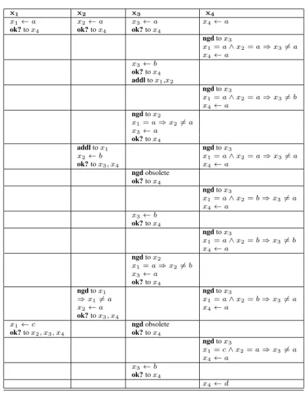
analyze how ABT runs on the three representations (since ABT may perform different executions, we follow one possible execution for each representation). ABT ordering isx1, x2, x3, x4and values are chosen lexicographically. The ABT trace on the three
representations appears in Figures 5-6.
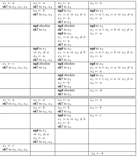
x1 x2 x3 x4
x1←a x2←a x3←a x4←a
ok?tox4 ok?tox4 ok?tox4
ngdtox3 x1=a∧x2=a⇒x36=a x4←a x3←b ok?tox4 addltox1,x2 ngdtox3 x1=a∧x2=a⇒x36=b x4←a ngdtox2 x1=a⇒x26=a x3←a ok?tox4 addltox1 ngdtox3 x2←b x1=a∧x2=a⇒x36=a ok?tox3, x4 x4←a ngdobsolete ok?tox4 ngdtox3 x1=a∧x2=b⇒x36=a x4←a x3←b ok?tox4 ngdtox3 x1=a∧x2=b⇒x36=b x4←a ngdtox2 x1=a⇒x26=b x3←a ok?tox4 ngdtox1 ngdtox3 ⇒x16=a x1=a∧x2=b⇒x36=a x2←a x4←a ok?tox3, x4 x1←c ngdobsolete ok?tox2, x3, x4 ok?tox4 ngdtox3 x1=c∧x2=a⇒x36=a x4←a x3←b ok?tox4 x4←d
Figure 5: Trace of ABT in the example, with three representations ofall-different: direct.
Direct representation: Variablesx1, x2, x3assign the first values in their domains,
informing repeatedly tox4, which backtracks repeatedly tox3, this tox2and this to x1, until valueais removed unconditionally fromD(x1). Then,x1takes valuecand
informsx4,x2andx3. They all have valuea. Then, x4 will backtrack onx3 which
will change its value toband will informx4, which will take valued. At this point, all
constraints are satisfied, the network is quiescent, a solution(c, a, b, d)has been found. Nested representation: Variablesx1, x2, x3assign the first values in their domains.
Variablex1 informs to variablesx2, x3 andx4. Variablex2 informs to variablesx3
x1←a x2←a x3←a x4←a
ok?tox2, x3, x4 ok?tox3, x4 ok?tox4
x2←b ngdtox2 ngdtox3 ok?tox3, x4 x1=a⇒x26=a x1=a∧x2=a⇒x36=a x3←a x4←a ok?tox4 ngdobsolete ngdobsolete ngdtox3 ok?tox3 ok?tox4 x1=a∧x2=b⇒x36=a ngdtox2 x4←a x1=a⇒x26=b x3←a ok?tox4 ngdtox1 ngdtox2 ngdtox3 ⇒x16=a x1=a⇒x26=b x1=a∧x2=b⇒x36=a x2←a x3←a x4←a ok?tox3, x4 ok?tox4 x1←c ngdobsolete ngdobsolete ngdtox3
ok?tox2, x3, x4 ok?tox3 ok?tox4 x1=a∧x2=a⇒x36=a
x4←a ngdobsolete ngdtox3 ok?tox4 x1=c∧x2=a⇒x36=a x3←b x4←a ok?tox4 ngdobsolete x4←d ok?tox4 x1←a x2←a x3←a x4←a
ok?tox2, x3, x4 ok?tox3, x4 ok?tox4
x2←b x3←b x4←b ok?tox3, x4 ok?tox4 ngdtox2 x4←c x1=a⇒x26=b x3←b ok?tox4 ngdtox1 ⇒x16=a x2←a ok?tox3, x4 x1←c ok?tox2, x3, x4 x4←d
Figure 6: Trace of ABT in the example, with three representations ofall-different: nested (top), binary (bottom).
backtracking messages to x2 andx3 respectively. At some point,x2 backtracks to x1removing unconditionally valuea. Then,x1takes valuec,x2andx3had already
valuea,x3 changes tob andx4 takes valued. The network is quiescent, the same
solution(c, a, b, d)has been found. Differences with the direct representation come from the number of constraints (1 in direct, 3 in nested) which determine the number of backtracking operations that could be performed simultaneously. In this sense, the nested representation does more work in parallel than the direct one.
Binary representation: All variables assign valueaand inform their lower priority agents in the binary constraints. Variablesx2andx3change tob, andx4changes toc.
There is a backtrack message fromx3tox2, which takes valuea, and another backtrack
fromx2 tox1, which now takes valuec. At this pointx4takes value d. Again, the
network is quiescent, the same solution(c, a, b, d)has been found. Differences with the direct and nested representation come from the number of constraints (1 in direct, 3
in nested, 6 in binary). This indicates the number of concurrent backtracks performed and also the number of variables which could adjust its value (the last variable in each constraint). In addition, the binary representation allows to backtrack to the real culprit of the inconsistency (to changex1 value fromatocbinary needs 2 backtrack only,
while nested needs 7 and direct needs 10).
4.3
Propagating Global Constraints
Independently of the way a global constraint is included into ABT, this algorithm can be enhanced by maintaining some form of local consistency during search. This was already investigated in [10], where limited/full forms of arc consistency (AC) were maintained during ABT execution for binary DisCSPs. While in [10] a limited form of AC causing unconditional deletions and full AC causing conditional deletions were considered, in this paper we maintain a limited form of GAC that causes unconditional deletions only. Clearly, this limited GAC, that from now on we call UGAC, is less pow-erful than full GAC. However, maintaining full GAC in the distributed context would cause a substantial load of extra communication which could overcome the benefits of domain pruning.
The basic idea is as follows: if during ABT execution agentself receives a NGD message justifying the removal of valuevwith a nogood with an empty left-hand side (see [2, 16, 10] for details),vcan be unconditionally deleted fromD(xself). A deletion onD(xself)is propagated maintaining UGAC on the constraints connectingxself to other variables, which may cause further deletions. Since the initial deletion is uncon-ditional, deletions caused by the propagation are also unconditional.
To maintain UGAC during ABT search, a number of modifications is needed over the basic ABT algorithm. They are:
• The domain of variables constrained withself by constraints inCself has to be
represented inself.
• Only the agent owner of a variable can modify its domain (i.e., onlyself can modifyD(xself)). If agentideduces that a value has to be deleted inD(xj), it does nothing because that deduction will be done injat some point.
• There is a new type of message, DEL, to notify of value deletions. DEL(self, k, v) –informing thatself removesvfromD(xself)– is sent fromself to every agent
kconstrained with it.
• All constraints are made GAC before ABT starts, by a suitable preprocess. Its pseudocode appears in Figure 7.
These changes do not modify ABT correctness and completeness. Regarding cor-rectness, the only UGAC action is to remove values that will not be in any solution, so correctness is maintained. Regarding completeness, we consider two cases:(i) remov-ing a value that is not currently assigned, and(ii)removing a value that is currently assigned. Case(i)trivially maintains completeness. Case(ii)also maintains com-pleteness, because the asynchronous ABT allows agents to change their value at any time.
procedureGAC-preprocess() /* quiescence: all constraints are GAC */
for eachC(T)∈ Cself doGAC(self, C(T));
while(¬end)do /*if end is true, empty domain detected */
msg←getMsg();
switch(msg.type)
Del:ValueDeletedPre(msg.sender,msg.value);
Stop:end←true;
procedureValueDeletedPre(j, a) /*jhas deleted valuea*/
D(xj)←D(xj)− {a};
for eachC(T)∈ Cselfs.t.xj∈TdoGAC(self, C(T)); procedureGAC(self, C(T))
ifrevise(xself, C(T))then
ifD(xself) =∅thensendMsg:Stop(system);
elseDelval←set of deleted values inD(xself)byrevise(xself, C(T))
for eachv∈Delvalandxk∈ST|C(T)∈Cself, k6=self do
sendMsg:Del(self, k, v);
Figure 7: GAC preprocess
Differences between ABT-UGAC and ABT are (see Figures 8-9):
• ABT-UGAC. It uses the DEL message, which notifies that a value has been
deleted in some domain. Ifself receives that message, it calls theValueDeleted
procedure.
• Conflict. Ifself accepts a NGD message containing a nogood with empty
left-hand side, it calls theDeleteValueprocedure.
• ValueDeleted(j, a). Agentjhas deleted valueafromD(xj)and sent a DEL
message toself. Agentself registers this in itsD(xj)copy, and enforces AC on all the constraints includingself andxj in their scope. If the value ofself is deleted in this process, theCheckAgentViewprocedure is called (looking for a new compatible value; if none exists it backtracks). Deletions inD(xself)are propagated.
• DeleteValue(a, j). Agentself must delete its currently assigned valuea
be-cause a nogood with empty left-hand side has been received from agentj. Value
ais deleted fromD(xself). If, as a consequence ofa’s deletion,D(xself) be-comes empty, there is no solution so a STOP message is produced. Otherwise,
a’s deletion is notified to all agents constrained withself exceptjvia DEL mes-sages, and the procedureCheckAgentViewis called.
• Backtrack. Afterself computes and sends a new nogood, it checks if its
left-hand side is empty. If so,self knows that the value that forbids the new nogood will be removed in the domain of the variable that appears in the right-hand side of the new nogood. Then self calls ValueDeleted, as if it had received a DEL message.
procedureABT-UGAC() /* ABT with unconditional GAC */
Γ = Γ−0 ∪Γ+0;Γ−= Γ−
0;Γ+= Γ + 0;
myV alue←empty;end←false;CheckAgentView();
while(¬end)do
msg←getMsg();
switch(msg.type)
Ok?:ProcessInfo(msg);AddL:SetLink(msg);
N gd:Conflict(msg);Stop:end←true;
new Del:ValueDeleted(msg.sender, msg.value);
procedureConflict(msg)
ifCoherent(msg.nogood,Γ−∪ {self})then new iflhs(msg.nogood)= emptythen
new DeleteValue(myV alue, msg.sender);
else
CheckAddLink(msg);
add(msg.nogood,myNogoodStore);
myValue←empty; CheckAgentView();
else ifCoherent(msg.nogood, self)then
sendMsg:Ok?(msg.sender, myV alue);
Figure 8: The ABT-UGAC algorithm (part 1); only procedures with new lines (new) with respect to ABT are shown.Γ−andΓ+are higher and lower priority agents
con-nected toself;Γ−0 andΓ+0 are those sets at the beginning of execution.
The difference that a global constraint instance C(T)makes with respect to any other generic constraint is when executing theGACprocedure. SinceC(T)has a well-defined semantics, it is often possible to generate specific propagators able to achieve the required level of local consistency polynomially whereas the generic propagator based on table lookups is exponential in the size ofT. In particular, we have imple-mented the popular flow-based propagator for theall-different constraint, following [25], which reduces propagation to matching theory.
Considering the running example of Figure 4 with the domainsD(x1) ={a, c, d}, D(x2) = D(x3) ={a, b},D(x4) ={a, b, c, d}, after applyingGAC-preprocess
on the direct or nested representations the following values are deleted:(x1, a)(x4, a)(x4, b).
However, this preprocess does not filter any value in the binary representation. From this on, ABT-UGAC on the direct and nested representations has a relatively simi-lar performance: the first value ofx1 andx2are part of the solution, a backtracking
fromx4 causesx3 to change to valueb (direct) whilex3 is able to adjust its value
tob(nested). ABT-UGAC on the binary representation does the same execution as described in Section 4.2.
4.4
Experimental Results
To evaluate the impact of global constraints in DisCSPs, we compare ABT with and without UGAC on random DisCSPs created as follows. We first generate random bi-nary instances using model B [26], and then add some global constraints. In model B,
new procedureValueDeleted(j, a) /*jhas deletedafromD(xj)*/ new D(xj)←D(xj)− {a};
new for eachC(T)∈ Cself s.t.j∈TdoGAC(xself, C(T));
new ifmyV alue6∈D(xself)then
new myV alue←empty;CheckAgentView();
new procedureDeleteValue(a, j) /*self deletesafromD(xself)*/
new D(xself)←D(xself)− {a};
new ifD(xself) =∅thensendMsg:Stop(system);
new else
new for eachk∈Γ0, k6=jdosendMsg:Del(self, k, a);
new CheckAgentView();
procedureBacktrack()
newN ogood←solve(myN ogoodStore);
if(newN ogood=empty)thenend←true;sendMsg:Stop(system);
else
sendMsg:N gd(newN ogood);
Update(myAgentV iew,rhs(newN ogood)←unknown);
new iflhs(newN ogood) =emptythen new ValueDeleted(rhs(newN ogood));
elseCheckAgentView();
Figure 9: The ABT-UGAC algorithm (part 2); only procedures with new lines (new) with respect to ABT are shown.Γ−andΓ+are higher and lower priority agents con-nected toself;Γ−0 andΓ+0 are those sets at the beginning of execution.
a random binary CSP class is characterized byhn, d, p1, p2i, wherenis the number of
variables,dis the domain size of each variable,p1is the problem connectivity defined
as the ratio of existing constraints andp2 is the constraint tightness expressed as the
ratio of forbidden value pairs. Hence, every instance containsp1·n(n−1)/2binary
constraints and each of them hasp2·d2forbidden value pairs. From a binary instance,
we can generate two types of benchmarks: theall-differentbenchmark and theatmost
benchmark. In theall-differentbenchmark, each binary instance includes 2all-different
constraints, each involving 5 randomly chosen variables. We also performed this exper-iment with 10 —instead of 2—all-differentconstraints per instance, obtaining similar results. Direct, nested and binary representations are used with theseall-different. In theatmostbenchmark, each binary instance includes 10atmost[k,v]constraints, each involving from 3 to 10 randomly chosen variables. The valuevwhose occurrences are bounded is also randomly chosen in the set of values occurring in domains and its max-imum number of occurrenceskis 1 or 2. Only direct and nested representations are used on theseatmostconstraints becauseatmostis not binary decomposable. In both benchmarks, since the order in which variables appear in the global constraint does not matter, we assumed the ABT priority order.
For theall-differentbenchmark, we have performed two experiments: sparseh20,5,0.2, p2i
and denseh20,5,0.7, p2i, wherep2varies between 0.1 and 0.9 in steps of 0.1. For
each experiment, we evaluate performance as the number of messages exchanged and the number of non-concurrent constraint checks (NCCCs) [27], considering the three representations. UGAC enforcing uses generic table lookups when testing binary
con-0.1 0.2 0.3 0.4 0.5 0.6 0.7 0.8 0.9
102
103
104
p2 messages (log scale) ABT(direct)
ABT(nested) ABT(binary) ABT−UGAC(direct) ABT−UGAC(nested) ABT−UGAC(binary) 0.1 0.2 0.3 0.4 0.5 0.6 0.7 0.8 0.9 103 104 p2 NCCCs (log scale) ABT(direct)
ABT(nested) ABT(binary)
ABT−UGAC(direct)
ABT−UGAC(nested)
ABT−UGAC(binary)
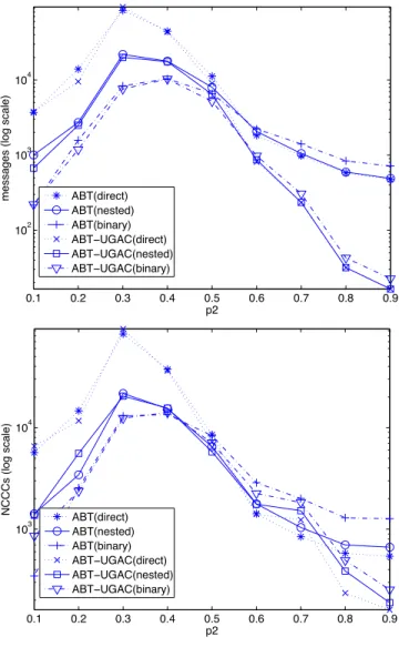
Figure 10: Results in #messages and NCCCs for theall-differentbenchmark described in the text. p1 = 0.2. Observe that for large values ofp2some lines superpose. Top
plot: ABT(direct) with ABT(nested), ABT-UGAC(direct) with ABT-UGAC(nested).
straints and it executes a special propagator when testing the globalall-different con-straints (as described in [25]). Each time this propagator is called it computes a max-imum matching in a graph; then, the NCCC counter increases in the number of nodes of that graph.
Results in number of exchanged messages and NCCCs appear in Figures 10-11, av-eraged on 100 instances per eachp2. Since sparse (p1= 0.2) and dense (p1= 0.7)
0.1 0.2 0.3 0.4 0.5 0.6 0.7 0.8 0.9
102
103
104
p2
messages (log scale) ABT(direct)
ABT(nested) ABT(binary) ABT−UGAC(direct) ABT−UGAC(nested) ABT−UGAC(binary) 0.1 0.2 0.3 0.4 0.5 0.6 0.7 0.8 0.9 103 104 105 p2 NCCCs (log scale) ABT(direct) ABT(nested) ABT(binary) ABT−UGAC(direct) ABT−UGAC(nested) ABT−UGAC(binary)
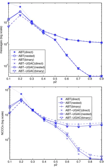
Figure 11: Results in #messages and NCCCs for the all-different benchmark de-scribed in the text. p1 = 0.7. Observe that for large values of p2 some lines
su-perpose. ABT(direct) with ABT(nested) with ABT(binary), ABT-UGAC(direct) with ABT-UGAC(nested) with ABT-UGAC(binary).
instances andp2 < 0.5(dense instances and p2 < 0.3, resp.) we observe that the
curve of plain ABT with a particular global constraint representation follows closely the curve of ABT-UGAC with the same representation. This shows that maintaining UGAC when constraints are loose does not pay off and it is the type of representation that makes the difference in efficiency. The most efficient representation is binary, fol-lowed by nested and finally direct representation. The direct representation causes
in-0.1 0.2 0.3 0.4 0.5 0.6 0.7 0.8 0.9 102 103 104 105 106 p2
messages (log scale)
ABT(direct) ABT(nested) ABT−UGAC(direct) ABT−UGAC(nested) 0.1 0.2 0.3 0.4 0.5 0.6 0.7 0.8 0.9 102 103 104 105 106 107 p2 NCCCs (log scale) ABT(direct) ABT(nested) ABT−UGAC(direct) ABT−UGAC(nested)
Figure 12: Results in #messages and NCCCs for theatmostbenchmark described in the text.p1 = 0.2. Observe that for large values ofp2some lines superpose. ABT(direct)
with ABT(nested), ABT-UGAC(direct) with ABT-UGAC(nested).
efficient chronological backtracking (which causes many useless messages —see ABT trace in Figure 5), and nested representation implies sending extra OK? messages. In this setting where not much pruning occurs, the binary decomposition appears as the most efficient, because although it sends many OK? messages, it performs backtrack-ing directly to the culprit.
For sparse instances andp2>0.5(dense instances andp2>0.3, resp.) the
maintain-0.1 0.2 0.3 0.4 0.5 0.6 0.7 0.8 0.9 102 103 104 105 p2
messages (log scale)
ABT(direct) ABT(nested) ABT−UGAC(direct) ABT−UGAC(nested) 0.1 0.2 0.3 0.4 0.5 0.6 0.7 0.8 0.9 102 103 104 105 106 p2 NCCCs (log scale) ABT(direct) ABT(nested) ABT−UGAC(direct) ABT−UGAC(nested)
Figure 13: Results in #messages and NCCCs for theatmostbenchmark described in the text.p1 = 0.7. Observe that for large values ofp2some lines superpose. ABT(direct)
with ABT(nested), ABT-UGAC(direct) with ABT-UGAC(nested).
ing UGAC is now the most discriminant element. The analysis of this fact is simple: for medium to high tightnesses, UGAC maintenance really decreases the size of the search space, so algorithms including UGAC terminate faster and thus require less messages (much less, observe the logarithmic scale) than plain ABT. On the relative performance of the three representations for global constraints, the less efficient representation is the binary, clearly dominated by the direct and nested ones, which practically use the same number of messages. We explain this as the combined effect of two facts: a high
num-ber of constraints (a singleall-differentbecomes a quadratic number of constraints in binary; a linear number of constraints in nested; one constraint in direct) and the fact that the problem has no solution. In the absence of solutions, ABT necessarily gen-erates nogoods to prove inconsistency and agents in binary will tend to send a higher number of NGD messages because they belong to more constraints than in the other representations. Some of these NGDs are useless and become obsolete.
Regarding NCCC, the observed pattern is similar to that observed for the number of messages. Differences among representations are due to the different number of constraints existing in each representation.
Results for theatmostbenchmark appear in Figures 12-13. We experimented with it becauseatmostis an example of non binary decomposable constraint. This explains why only the direct and nested representations are reported. Evaluation was similar to the one done on theall-differentbenchmark: two experiments: sparseh20,5,0.2, p2i
and denseh20,5,0.7, p2i, wherep2varies between 0.1 and 0.9 in steps of 0.1,
count-ing the number of messages exchanged and the number of non-concurrent constraint checks (NCCC) on the available representations. Results are averaged on 100 instances perp2.
The number of exchanged messages shows a similar pattern to the one observed in theall-differentbenchmark. For sparse instances andp2 < 0.5 (dense instances
andp2 < 0.3, resp.) we observe that UGAC has no much effect and the dominant
factor is the representation of the global constraint: as in theall-differentbenchmark, the direct representation is much worse than the nested one. For sparse instances and
p2 > 0.5 (dense instances and p2 > 0.3, resp.) the situation changes. As in the
case of theall-differentbenchmark, maintaining UGAC becomes the main reason for efficiency, more important than the type of representation of the global constraints. Thus, ABT curves are closely related, while ABT-UGAC curves are also closely joined. The explanation of this fact is the same as in theall-differentbenchmark: For medium to high tightness, UGAC maintenance really decreases the size of the search space, so algorithms including UGAC terminate faster and require much less messages to explore that space than plain ABT.
Regarding NCCC, they show a pattern similar to the number of messages. Differ-ences among representations are due to the different number of constraints existing in each representation.
5
Global Cost Functions in DCOP
In this section we consider the introduction of global cost functions in distributed con-straint optimization problems. The section is organized exactly as Section 4.
5.1
Representing Global Cost Functions
We consider three different ways to model the inclusion of a global cost function in DCOPs. The user chooses one of the three representations and the solving is done on that representation.
The first way is the direct representation. An instanceC(T)of a global cost func-tionCis posted as a single cost function. Only the last agent (among the agents inT) in the branch of the pseudo-tree evaluates the cost function.
In the DisCSP case, we had the nested representation whenC was contractible. Contractibility is a notion also defined in the optimization case. Unfortunately, the technique of the nested representation used for DisCSPs no longer works. When we create copies of the global cost functionC(T)on subsets of the variables inT, costs are duplicated and the model remains no loger equivalent. Take for instance the global cost functionsoft-all-different(x1, x2, x3, x4)and its nested representationS = {soft-all-different(x1, x2),soft-all-different(x1, x2, x3),soft-all-different(x1, x2, x3, x4)}.
Consider the assignmentx1 = a, x2 = a, x3 = b, x4 = c. The cost of assigning x1=a, x2=awill be counted in all three cost functions in the nested representation,
leading to a higher cost than that in the originalsoft-all-different(x1, x2, x3, x4)global
cost function, thus losing equivalence. However, we still have the interesting property that each cost function inStaken separately produces costs that never exceed the cost of the original global cost function. This property can be used to still use the nested representation in DCOPs provided that we slightly modify the algorithms so that when an agent receives costs from several cost functions from the same nested representation, it does not sum them but takes their maximum.
Finally, the binary representation works the same as in DisCSPs. IfC is binary decomposable, instead ofC(T), the binary decomposition ofC(T)is included in the problem.
5.2
Searching with Global Cost Functions
We have extended the distributed search algorithm BnB-ADOPT+ [22] to support
global cost functions with a direct, nested and binary representations. Some modifi-cations of the original algorithm are needed, explained below.
In the case of the binary representation, there is no need for any modification: BnB-ADOPT+works as usual since the global cost function has been expressed as a set of binary cost functions. For the nested and direct representations, we apply the following modifications:
1. Every agentself keeps a global cost function set with all the global cost functions in whichself is involved. Every global cost functionC(T)implicitly contains the agents involved inT (neighbors ofself). For some cost functions, additional information can be stored. For example, for thesoft-at-most[k,v]cost function, parametersk(number of repetitions) andv(domain value) are stored.
2. During the search process, every timeself needs to evaluate the cost of a given valuev, all local costs are aggregated. Binary cost functions are evaluated as usual, and global cost functions are evaluated according to its violation measure. 3. VALUE messages are sent to children and pseudo-children involved in any kind —binary or global— of cost functions. In the case of direct representation, VALUE messages are sent only to the deepest agent in the DFS tree involved in the global cost function (no VALUES are sent to intermediate agents because
(1)procedureCalculateCost(value)
(2) cost=cost+BinaryCostWithValue(value); (3) cost=cost+GlobalCostWithValue(value);
(4) returncost;
(5)functionBinaryCostWithValue(value)
(6) for each(xi,di)∈contextdo
(7) binaryCost=binaryCost+C(xi, self)(di, value);
(8) returnbinaryCost;
(9)functionGlobalCostWithValue(value)
(10) cost =0;
(11) for eachglobal∈globalCtrSetdo
(12) for each(xi,di)∈contextdo
(13) ifxi ∈global.varsthenglobalContext.add(xi, di);
(14) ifglobalContext.size==global.vars.sizethen //self last evaluator
(15) cost=cost+EvalGlobal(global,globalContext∪(self,value)); (16) else //self is an intermediate agent in the restriction
(17) ifDIRECTrepresentationthencost=cost+ 0;
(18) ifN EST EDrepresentationthen
(19) for eachxi∈global.varsdo
(20) iflowerGlobalEvals.contain(xi)thencost=cost+ 0;
(21) elsecost=cost+EvalGlobal(globalContext∪(self,value));
(22) returncost;
(23) functionEvalGlobal(global, varAssignments)
(24) returnglobal.µ(varAssignments);
Figure 14: Aggregating costs of binary and global cost functions.
they are not able to evaluate the global cost function). In the case of nested representation, VALUE messages are sent to all children and pseudo-children involved in the global cost function, since they are all able to evaluate it. 4. COST messages include a list of all the agents that have evaluated a global cost
function. This is done to prevent duplication of costs and is explained in the next paragraphs.
Figure 14 shows the pseudocode for cost aggregation of binary and global cost functions in BnB-ADOPT+(lines 1-4). Binary costs are calculated as usual, aggregat-ing all binary costs evaluated onself value and the assignments of the current context (lines 5-8). Global costs are calculated in lines 9-20. Although there is no need to separate binary cost aggregation from global cost aggregation, we have presented them in separate procedures for a better understanding of the new modifications.
For every global cost function of the global cost function set (globalCtrSet)self
creates a tuple with their assignment in the current context (globalContext, lines 11-13). Ifself is the deepest agent in the DFS tree (taking into account the variables involved in the global cost function) thenself evaluates the cost function (lines 14-15). Ifself is an intermediate agent, it does the following. If representation is direct,
representation is nested, it requires some care, as we said when presenting the nested representation. A nested global cost function is evaluated more than once by interme-diate agents and if these costs are simply aggregated duplication of costs may occur. To prevent this, COST messages include the set of agents that have evaluated their global cost functions (lowerGlobalEvals). When a COST message arrives,self knows which agents have evaluated their cost functions and contributed to the lower bound. If some of them appear in the scope ofC, thenself does not evaluate this cost function (lines 18-21). By doing this, the deepest agent in the DFS tree evaluating the global cost function precludes any other agent in the same branch to evaluate the cost func-tion, avoiding cost duplication. Preference is given to the deepest agent because is the one that receives more value assignments and can perform a more informed evalua-tion. When bounds coming from a branch of the DFS are reinitialized (this happens under certain conditions in BnB-ADOPT, for details see [21]), the agents in the set
lowerGlobalEvalslying on that branch are removed.
Finally, a procedure for evaluating the global cost functions according to its viola-tion measure is presented in lines 23-24.
5.3
Propagating Global Cost Functions
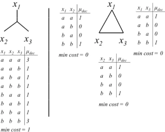
When introducing soft local consistency, the solving process is improved. The quality of the bounds obtained as the result of applying local consistency is often better when the problem contains global constraints than when it contains an equivalent binary for-mulation. For example, consider the case of thesoft-all-different(x1, x2, x3)with
vio-lation measureµdecand its equivalent binary formulation: {soft-all-different(x1, x2), soft-all-different(x2, x3),soft-all-different(x1, x3)}with the domain set{a, b}for every
variable (Figure 15). If UGAC is applied on the global formulation it can be inferred a lower bound of 1 for the optimal solution. Since there are three variables and only two domain values, any ternary tuple (with a combination ofx1, x2, x3values) will cost at
least 1 (Figure 15, left). However in the binary formulation we can only infer a lower bound of 0, if looking independently at every binary tuple (Figure 15, right).
Specific propagators exploiting the semantics of global cost functions has been proposed in the centralized case. These propagators allow to achieve the generalized arc consistency level more efficiently than using generic propagators. In both cases —binary or global cost functions— soft local consistency is based onequivalent pre-serving transformationswhere costs are shifted from binary/global cost functions to unary cost functions.
These same technique can be applied in distributed COP. We project costs from binary and global cost functions to unary cost functions and finally project unary costs toCφ. After binary/global projections are made, agents check their domains searching for inconsistent values. For this, some modifications are needed:
• The domain of neighboring agents (agents connected withself by cost functions) are represented inself.
• A new DEL message is added to notify value deletions.
x1 x3 μdec a a 1 x1 x2 μdec a a 1
x
1x
1 a a 1 a b 0 b a 0 a a 1 a b 0 b 0 b a 0 b b 1 b a 0 b b 1x
2x
3 x x x μx
2x
3 x2 x3 μdec a a 1 x1 x2 x3 μdec a a a 3 b 1min cost = 0 min cost = 0 a a 1 a b 0 b 0 a a b 1 a b a 1 b a 0 b b 1 a b b 1 b a a 1 b a b 1 b b a 1 min cost = 0 b b b 3 min cost = 1
Figure 15: (Left)soft-all-different(x1, x2, x3)withµdecviolation measure; (right) its binary decomposition
Following the technique proposed in [11], we maintain the GAC consistency level during search, but performing only unconditional deletions, so we call it unconditional generalized arc consistency (UGAC). An agentself deletes a valuevunconditionally
if this value is guaranteed to be sub-optimal and does not need to be restored again dur-ing the search process. Ifself contains a valuevnot NC (C(self)(v) +Cφ >>) then
vcan be deleted unconditionally because the cost of a solution containing the assign-mentself = vis necessarily greater than>. We also detect unconditional deletions in the following way. Let us consider agentself executing BnB-ADOPT+. Suppose
self assigns value v and sends the corresponding VALUE messages to children and pseudo-children. As response, COST messages arrive. We consider those COST mes-sages whose context is simply(self, v). This means that the bounds informed in these COST messages only depend onself assignment (observe that therootagent always receives such COST messages). If the sum of the lower bounds contained in those COST messages exceeds>, v can be deleted unconditionally because the cost of a solution containingself =vis necessarily greater than>.
As in [11], messages include information required to perform deletions, namely>
BnB-ADOPT+-UGAC messages:
VALUE(sender,destination,value,threshold,>,Cφ)
COST(sender,destination,context[],lb,ub,subtreeContr agents contributing lb)
TERMINATE(sender,destination,emptydomain)
DEL(sender,destination,value)
Figure 16: Messages of BnB-ADOPT+-UGAC. New parts wrt. BnB-ADOPT+ are underlined.